Functional Parametric Elasto-Dynamics for Efficient Multicomponent Design

Abstract

In industrial settings, engineering products are often divided into separate components for detailed conception. They often require iterative corrections between different designers/teams to optimize the final product with all components assembled into a system. This article proposes a surrogate modeling approach with functional descriptions of parts in the model and aims to accelerate the design and optimization phase in real projects. The approach is applied to a vibration problem of a two-component plate structure, where the model estimates the dynamic behavior of the assembled system when only the properties of each individual part are available. A database is built using high-fidelity numerical simulations, and neural-network-based regressions provide reliable predictions on unseen data.

1. Introduction

When designing a complex engineering product, such as a car, a drone, an airplane, etc., the conception of each component is performed in parallel and is synchronized regularly among different teams. During the optimization phase, each team continues to optimize its parts design, aiming for the improvement of the overall product performance. Such a process is in general lengthy and requires many iterations. Moreover, the optimized solution proposed after a complete study could be invalid when integrating modifications from other teams. Therefore, there exists a consistent demand for novel approaches to enable agile consideration of design changes in the ongoing project, thus accelerating the optimization process.

Recently, the concept of surrogate models has been largely investigated. These models are employed with some parameters, such as material properties and shapes, and are then used to predict the system’s response under certain loading and environmental conditions. The construction of these parametric models can be data-driven and is usually combined with model order reduction methods and advanced machine learning techniques. Such an approach can be especially useful for optimization procedures because reduced models perform faster than high fidelity simulations, which are often computationally demanding. Various applications can be found for manufacturing process optimization [1], industrial product designs for turbines [2], antenna structures [3], etc. In most cases, the inputs for surrogate models are design parameters that rely on detailed numerical models; however, such inputs are not fully convenient in some industrial contexts.

Imagine a hypothetical situation in which two teams are involved in an industrial design project: team 1 is responsible for a subset of the total system containing multiple parts, and team 2 deals with the rest. The two teams work independently and asynchronously for their subsystem design and optimization. They only coordinate on specific pointy meetings as planned in the project schedule. Teams do not always dispose of the latest updated design of the other ones. Thus, they can only use the last available version to evaluate the performance of their own design. In the early stage of the project, each team works with standard specifications from another team and they evaluate the performance while assuming that the latter will achieve its objectives. At fixed project checkpoints, the specifications will be replaced by realistic updated proposals. To ease the negotiation between teams, each one must propose novel objectives for the others and represent the other subsystem by a set of easily manipulable design parameters. The parameters have to be of a functional nature, instead of relying on the detailed design, such as the thicknesses of certain parts, as no numerical conception is fixed at that moment.

Classical approaches with conception parameters cannot adapt to the described situation, and this inspires the idea of constructing surrogate models with functional design parameters. Conception parameters, such as thickness, local shape and material properties, are elementary for the definition of numerical models. However, functional parameters can be viewed as consequences of the defined designs. Reversely, the optimization based on functional parameters could also guide the search for optimal design conception.

In vibroacoustics, the modal representation of parts and subsystems perfectly match the role of functional parameters for surrogate modeling. It is known that vibration modes are commonly used to characterize the behavior of designed parts, including eigenfrequencies and eigenvectors. They encapsulate all geometrical information of the models as well as the impact of usual design parameters, while helping to improve the description of subsystems’ behavior.

Many existing studies focus on the decomposition of systems and evaluation of the global performance based on separate parts. Either analytical means or numerical simulations are used, while a few have mentioned the usage of functional parameters. The difficulty of evaluating the dynamic behavior of the whole system with assembled parts has been widely acknowledged. In fact, the assembled system performance is not a simple juxtaposition of individual behaviors of parts [4]. Moreover, simulations for the whole system are usually costly and time-consuming, affecting different departments working asynchronously. Thus, it is undesirable in an industrial context where decisions should be timely [5,6]. Simulations may not be even feasible in the early stage of the project, as described in a previous paragraph. Analytical methods are preferred in such situations, as they allow a large number of iterations and trials within a short period of time [5]. Different studies have focused on the vibration analysis of coupled plates, aiming to derive analytical solutions for cases of interest [7,8,9,10,11]. However, analytical solutions are rarely available and hard to derive for large-scale industrial structural systems. Numerical simulation appears thus as an appealing resort to analyze the vibration response of assembled components [12]. In [13], the authors used a finite element modeling of adhesive bonded plates to investigate the effect of different model parameters on the global system mode shapes. However, numerical simulation is generally time-consuming in industrial settings. Another recent interesting approach is to build a surrogate model of an assembled system to predict the behavioral change of the final product as a function of changes in any of its components’ properties. In [14], the authors built a surrogate model using artificial neural networks to predict the natural frequency of an adhesive bonded double-strap joint, as well as the loss factor. The surrogate model was later leveraged to optimize the joint mass.

In this paper, we focus on the vibration problem and propose a novel approach using functional parameters to predict the dynamic behavior of the whole structural system based on physical information of the system’s components. This work is a first attempt to predict a final assembled system behavior, based on the functional properties of its individual components. Our approach allows real-time estimation of the final system response, for any combination of its components’ functional properties, such as mode shapes and eigenvalues. Such an approach was never addressed until now, to the best knowledge of the authors. The article starts with a brief introduction of surrogate modeling with neural network regression in Section 2. It follows by the problem description and a review of data generation in Section 3. Results of the surrogate model are shown in Section 4, and the article ends with some conclusions addressed in Section 5.

2. Surrogate Modeling with Neural Network

Consider the vibration problem of a structural system composed of different parts. Each part has its own design that is defined using a number of design parameters, such as part thickness, local part curvature, material properties, etc. Here, the surrogate modeling approach proposes to use a functional description of each part design instead of the usage of design parameters as considered in usual approaches.

The modeling framework in this study is to predict global system behaviors, using individual modal inputs of the different parts involved in the system. The inputs are the first main eigenfrequencies $\{{\mathbf{\omega }}^{\mathbf{1}},{\mathbf{\omega }}^{\mathbf{2}},\cdots ,{\mathbf{\omega }}^{\mathbf{P}}\}$ of all P parts. For each part i, the feature ${\mathbf{\omega }}^{\mathbf{i}}$ is a vector that contains the eigenfrequency values related to the N first modes. The surrogate model computes physical quantities of interest $\mathbf{y}$, including the eigenfrequencies of the whole system and maximal displacement of the system at these eigenfrequencies, as well as the dynamic response of displacement amplitudes within a frequency interval. Neural-network-based regressions help to find the function h relating inputs and outputs. The surrogate modeling can thus be written as

$$\mathbf{y}=h({\mathbf{\omega }}^{\mathbf{1}},\cdots ,{\mathbf{\omega }}^{\mathbf{P}})$$

(1)

Once h is available, it can be used to optimize conception parameters of each part, such as the geometries and materials. Moreover, a wide range of variation is possible, as long as the individual eigenfrequencies of the whole assembled system are in the range of the training set.

3. Problem Context and Data Generation

The proposed surrogate modeling framework will be tested on a two-component plate problem, where a loading is applied on one part of the structure, and the performance of the whole system will be evaluated on a second part. The defined problem on the plate model can be seen as an simplified representation of vehicle vibroacoustic studies: vibrations from engines excite the engine supporting structure, and we monitor vibration behaviors on frame structures surrounding the cabin that could result in unwanted vehicle interior noises.

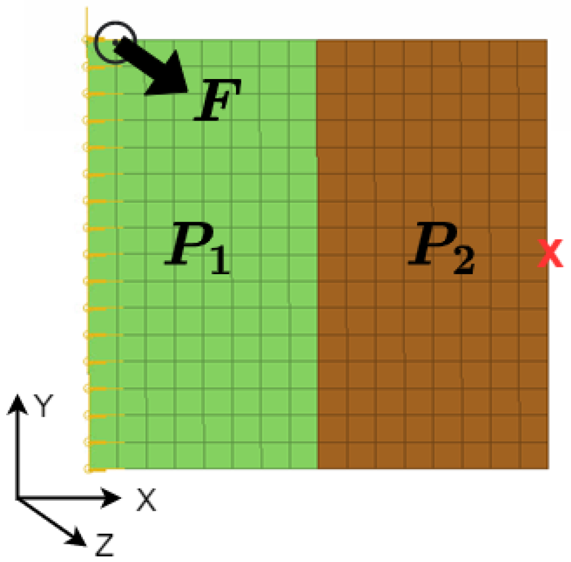
In the present analysis, we consider a plate [0, 0.5] × [0, 0.5] composed of two components, as depicted in Figure 1. The left edge is fixed, and a constant unit nodal force $F=1$ N is applied along the positive z direction at location $x=0.03125$ N, $y=0.5$ m. The whole plate is composed by one material of density $\rho =2.768\times {10}^3$ kg/${\mathrm{m}}^3$, Poisson’s ratio $\mu =0.3$ and Young’s modulus $E=$ 68.95 GPa. A structural damping ratio of $3\%$ is applied to the whole structure.

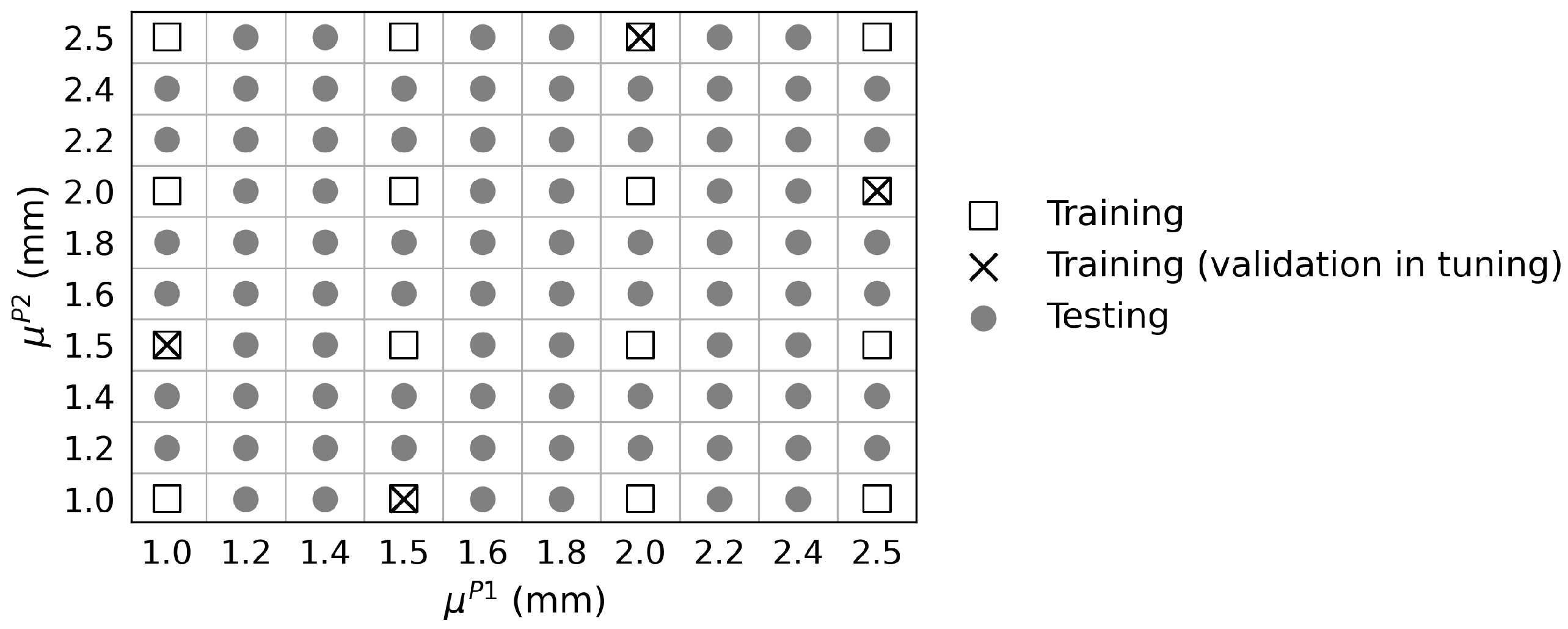
In the plate model, the two parts are respectively denoted by $P_1$ for the left and $P_2$ for the right. A full factorial design of experiments (DOE) is used to vary two factors, $P_1$ and $P_2$ thicknesses ${\mu }^{P_1}$ and ${\mu }^{P_2}$, at ten different levels between [1, 2.5] mm, resulting in ${10}^2=100$ configurations to form our database. The discrete thickness values of ten levels can be seen later in the figures presenting the separation of training and testing sets for model construction and evaluation. The 2D finite element model is meshed with 256 quadratic elements.

Numerical simulations are performed using Nastran software. For each configuration, modal analyses (MSC/NASTRAN SOL103) are launched separately for both parts $P_1$ and $P_2$ to retrieve their modal results. Calculations for part $P_1$ are conducted with its boundary condition on the left edge. Eigenfrequencies ${\mathbf{\omega }}^{{\mathbf{P}}_{\mathbf{1}}}$ are saved for the first $N^{P_1}$ non-rigid modes, with $N^{P_1}$ the number of modes. Part $P_2$ is set as free of constraints and similarly, modal data ${\mathbf{\omega }}^{{\mathbf{P}}_{\mathbf{2}}}$ is saved for its first $N^{P_2}$ non-rigid modes. These results will be used later as an input for the surrogate model. Eigenvalue analysis is also performed on the whole assembled system to calculate eigenfrequencies ${\mathbf{\omega }}^{{\mathbf{P}}_{\mathbf{1}}+{\mathbf{P}}_{\mathbf{2}}}$ of its first $N^{P_1+P_2}$ modes, which is one of the physical quantities to be predicted by the surrogate model. In addition, modal frequency response analysis (MSC/NASTRAN SOL111) is conducted for each configuration to obtain the z-component displacement amplitudes ${\mathbf{u}}_{\mathbf{z}}\left(f\right)$ for frequencies $f\in$ [5, 100] Hz with a step of 1 Hz. Moreover, the displacement amplitudes at natural frequencies of the assembled system ${\mathbf{u}}_{\mathbf{z}}\left({\mathbf{\omega }}^{{\mathbf{P}}_{\mathbf{1}}+{\mathbf{P}}_{\mathbf{2}}}\right)$ are computed. Here, the surrogate model aims at predicting the displacement output at one specific prescribed point: the middle node on the right edge of the plate, at location $x=0.5$ m, $y=0.25$ m, as marked by the red cross in Figure 1. The procedure generalizes for computing quantities in any arbitrary point.

The choice of the number of modes depends on the main frequency range of interest for dynamic response analysis. In this study, this frequency range is fixed up to 100 Hz. Thus, the modal basis should include all modes with eigenfrequencies under 150 Hz, generally at least 1.5 times the upper limit of 100 Hz. The configuration with thicknesses ${\mu }^{P_1}={\mu }^{P_2}=$ 1 mm presents the highest number of modes within the 150 Hz range, and it has respectively $N^{P_1}=$8 modes for $P_1$, $N^{P_2}=$9 modes for $P_2$ and $N^{P_1+P_2}=11$ modes for the assembled system. Even though for certain configurations the 8^th or 9^th eigenfrequency could be around 230 Hz, the same number of modes is considered for all inputs to ensure a consistent dimension of inputs and outputs for the surrogate model. Figure 2 shows the respective eigenfrequencies of $P_1$ and $P_2$ of one configuration as an example.

Figure 3 shows the distribution of the eigenfrequencies of the system for all 100 configurations in the database. It is clear that there exist large variations of eigenfrequency values for modes of a higher order, while the distribution of lower eigenfrequencies is relatively narrow. Thus, the prediction for lower eigenfrequencies will be easy, as the variations among different configurations are small, but the prediction for higher eigenfrequencies will still be challenging. 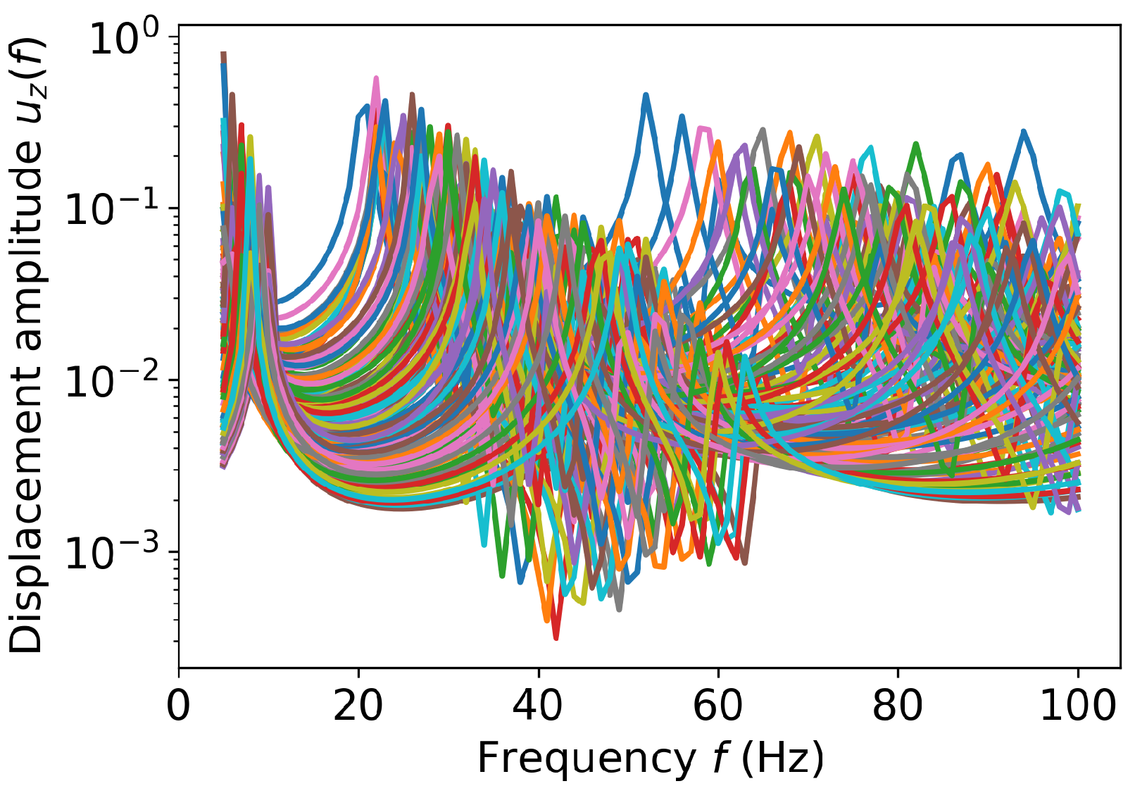Figure 4 shows the z-component displacement amplitudes for all configurations. These displacement profiles present noticeable variations in amplitudes and shifted locations of the natural frequencies, showing that the construction of surrogate models is not a simple task.

4. Results and Discussions

Surrogate models in this study are all constructed with neural network regressions, and the network structure will be illustrated later. The three models have same inputs, the eigenfrequencies of $P_1$ and $P_2$. These values are all respectively transformed to have zero mean and normalized by the maximum absolute value on the training set. Same scalars are then applied to data in the testing set. Similarly, in each prediction task, the physical quantity of model output is also transformed to have zero mean and normalized by the maximum absolute value for training and is scaled for testing set. Normalization for inputs and outputs is essential for efficient neural network training.

4.1. Prediction of Eigenfrequencies of the Assembled System: Model ${\mathcal{H}}_1$

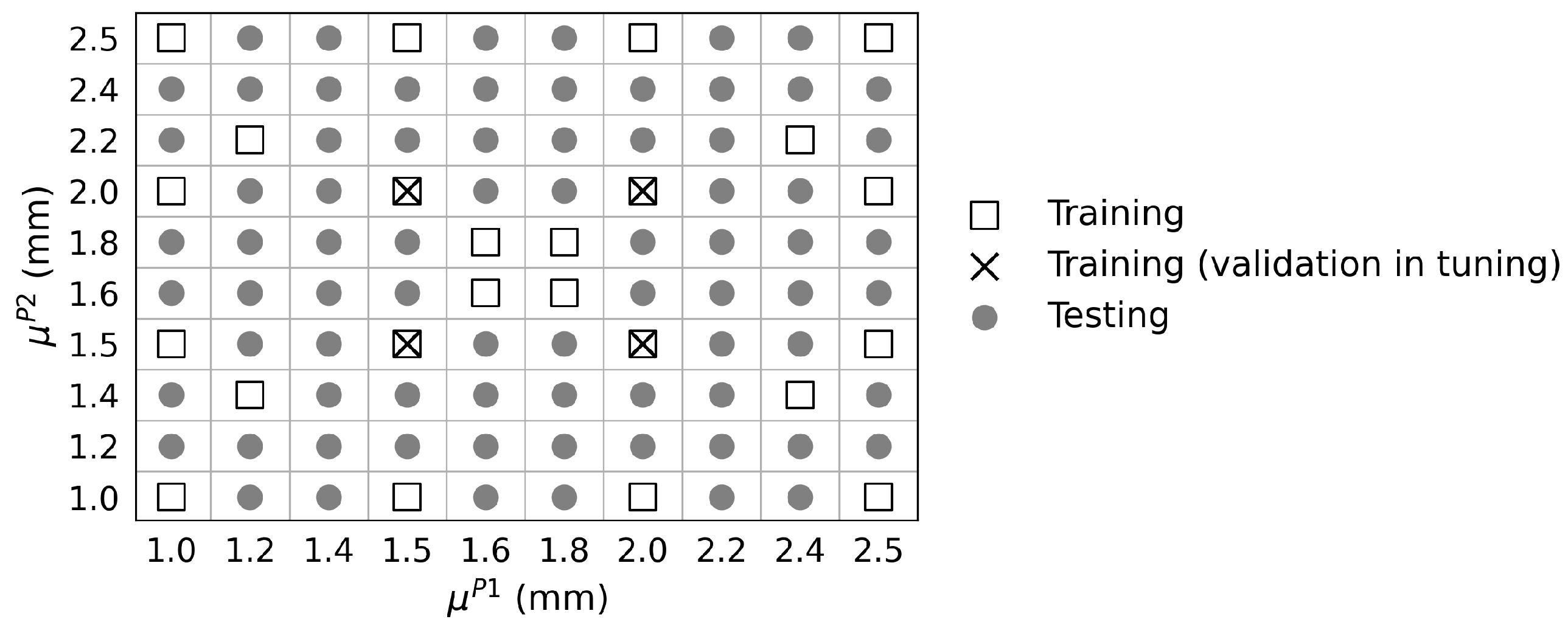
In this section, the objective of surrogate modeling is to predict the eigenfrequencies of the assembled system based on those of the constitutive parts. The model will be noted as ${\mathcal{H}}_1$. Given the results of 100 configurations in the database, 16 samples are chosen for the training set, and the rest are used as testing set for the surrogate model evaluation. Figure 5 shows the distribution of the 16 selected samples in the parametric space that includes all extreme sampling points at the 4 corners and some intermediate ones. There are 4 of the 16 selected samples that will be used as validation set for network tuning test, later explained in this section.

Note that for the studies in the present paper, no extra investigations have been conducted to find out a minimum size of the training set. It is possible that, with an appropriate optimal DOE, the number of necessary samples for training can be further reduced while guaranteeing an equivalent level of accuracy.

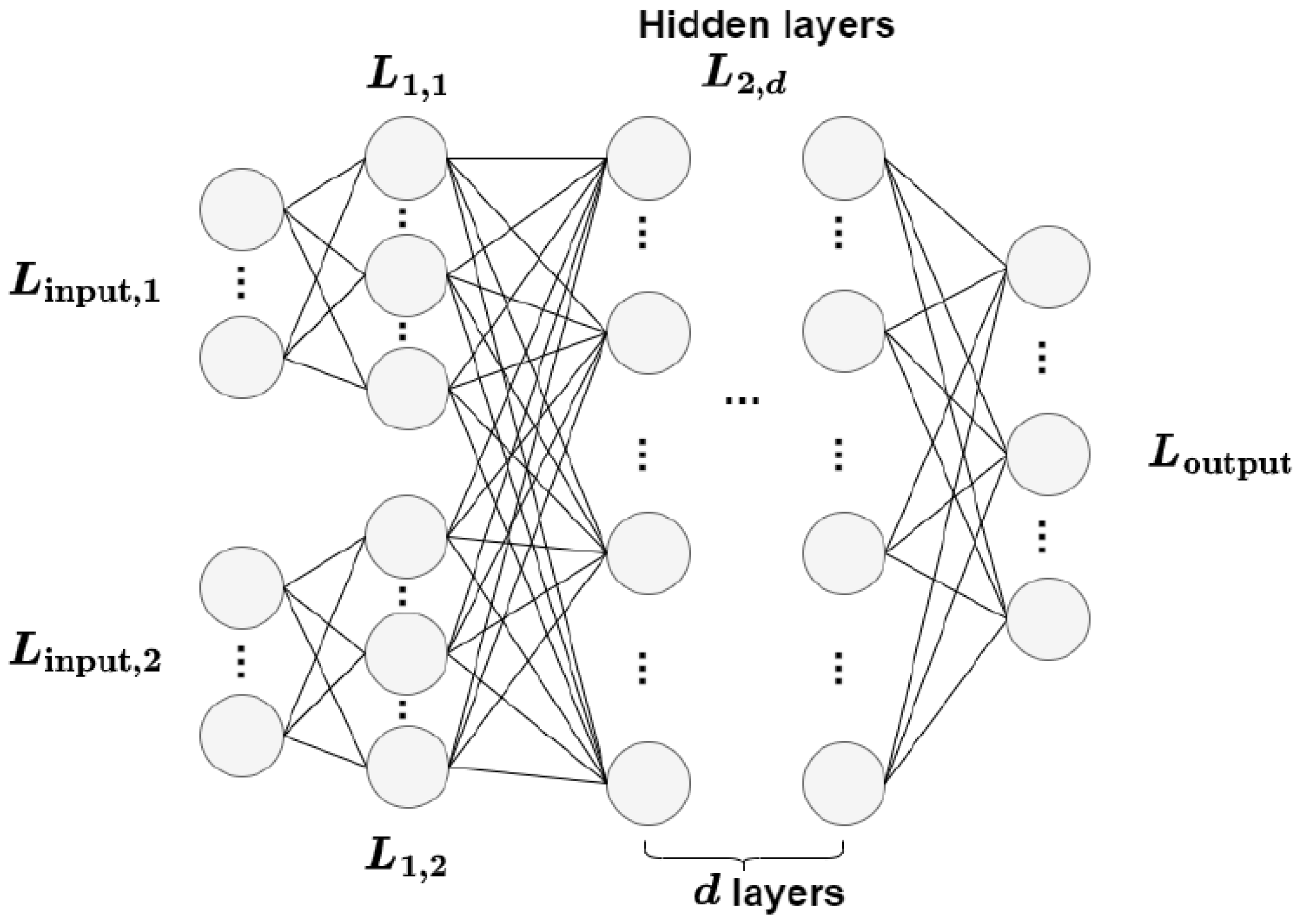
A usual multi-layer fully connected network is considered for this task, and its architecture is given in

Table 1. Structure of the neural network.

Layer	Layer Dimension	Activation 1	Initializer 2
$L_{\mathrm{input},1}$	8	-	-
$L_{\mathrm{input},2}$	9	-	-
$L_{1,1}$	8 × k	tanh	GlorotNormal
$L_{1,2}$	9 × k	tanh	GlorotNormal
$L_{2,d}$	D	elu	HeNormal
$L_{\mathrm{output}}$	11	linear	-

¹ In the Activation column, tanh stands for the hyperbolic tangent activation function, ^elu stands for the exponential linear unit and linear means linear activation with scalar coefficient 1. ² In the Initializer column, GlorotNormal and HeNormal are two network weight initialization methods, chosen in coherence with the layer’s activation function.

and displayed in Figure 6. The network starts with two separate input layers of dimension 8 for ${\mathbf{\omega }}^{{\mathbf{P}}_{\mathbf{1}}}$ and of dimension 9 for ${\mathbf{\omega }}^{{\mathbf{P}}_{\mathbf{2}}}$. Then each input layer is fully connected to layers $L_{1,1}$ and $L_{1,2}$, with a dimension increased by k to accommodate data into a higher dimension space. Outputs from $L_{1,1}$ and $L_{1,2}$ layers are concatenated into a vector with a dimension equal to $17\times k$, and it is fully connected to subsequent layers $L_{2,d}$ with D neurons. The last hidden layers is connected to an output layer with dimension 11, equal to the dimension of ${\mathbf{\omega }}^{{\mathbf{P}}_{\mathbf{1}}+{\mathbf{P}}_{\mathbf{2}}}$. The mean squared error (MSE) is used in the loss function, the same choice for all models in the rest of the paper.

Network tuning helps to fix network hyperparameters: factor k between input layers $L_{1,1}$ and $L_{1,2}$, number of hidden layers d and hidden layer dimension D. The tuning is performed with 12 of the 16 selected samples and the remaining 4 samples are used for validation, as already shown in Figure 5. Error comparison of different network setups is given in

Table 2. Error comparison of different networks in model ${\mathcal{H}}_1$ tuning tests. The network 3 (in red) is the final choice.

No.	Dimension Multiplication Factor k	Number of Hidden Layers d	Hidden Layer Dimension D	Trainable Parameters	Training MAPE	Validation MAPE
1	5	1	50	5671	3.330%	2.427%
2	5	1	100	10,521	1.576%	1.919%
3	5	1	200	20,221	1.082%	1.407%
4	10	1	100	19,831	1.651%	1.818%
5	5	2	100	20,621	1.206%	1.726%

, with mean absolute percentage error (MAPE) as the error indicator. Its definition is given by

$$\mathrm{MAPE}=\frac{1}{N}\sum _{n=1}^N\left|\frac{A_n-{\widehat{A}}_n}{A_n}\right|$$

(2)

where N is the number of samples in either training or validation set. A represents the reference output value and $\widehat{A}$ the predicted value by the model.

For all tuning tests, networks are trained with a batch size of 12, involving all training samples. All networks are supposed to be trained for a maximum of 5000 epochs, while an early-stopping scheme is implemented. The early stopping keeps track of the validation loss and saves the best model when the validation loss stops decreasing in order to avoid overfitting on the training set.

Results of networks No. 1 to No. 3 in Table 2 show that the increase in hidden layer dimension can effectively reduce the validation error. Networks No. 4 and No. 5 are conducted with similar level of trainable parameter number as network No. 3. It can be seen that, for this task, increasing factor k or involving more hidden layers is less helpful for model improvement compared to an increase in hidden layer dimension. The final choice is network No. 3, which presents the best compromise between the precision on validation set and the model complexity.

A neural network with the chosen hyperparameters is finally trained with a batch size of 16 for all 16 samples in training set. Here, the early-stopping scheme is not applied, as the 16 samples are all used for training with no indication of validation loss to monitor the training process. The convergence curve of the training stage over 5000 epochs is shown in Figure 7, and the loss on the testing set is also plotted for each epoch, showing that the model does not overfit on training. Note that the MAPE displayed in this figure is calculated for the gap between normalized reference values and the predicted ones during the model training, and thus is not comparable with other MAPEs calculated with values scaled back to original intervals.

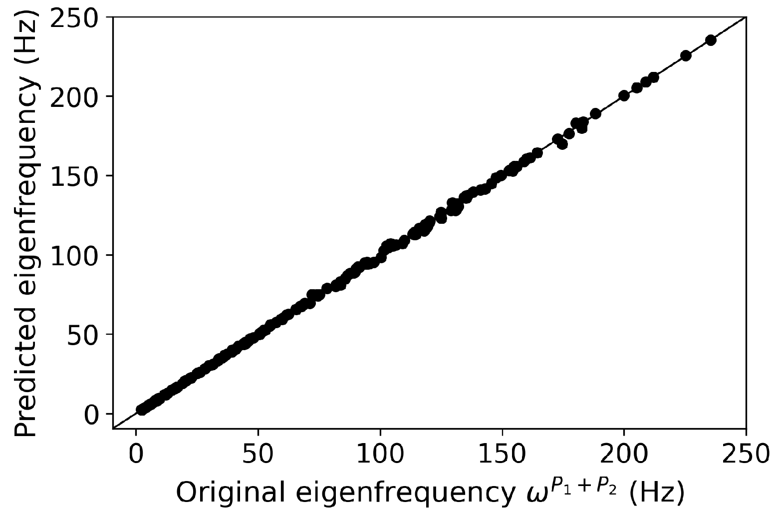
Figure 8 displays the predicted output values versus the reference ones of the training set. The same plot is presented for the testing set of 84 samples in Figure 9a. The surrogate model produces satisfying predictions for the testing set, with MAPE $=1.025\%$. Figure 9b,c display the results of two samples with the smallest and largest MAPE for the prediction of 11 eigenfrequencies. Even for the one with maximum error, the predictions of the surrogate model approximate very accurately the reference values.

4.2. Prediction of Displacement Amplitude at Natural Frequencies of the Assembled System: Model ${\mathcal{H}}_2$

The objective here is to predict the amplitude of the z-component of displacement at the natural frequencies of the assembled system. With the success of model ${\mathcal{H}}_1$ in locating the whole system eigenfrequencies, the next step is to see whether the neural network approach can capture the nodal displacement amplitudes at these key frequencies. This physical quantity deserves special attention, as it usually quantifies behaviors for structure vibration problems.

For this task, the neural network structure is same as model ${\mathcal{H}}_1$, already shown in Table 1, since the output dimension is also 11. Preliminary tests indicate that the training for this new model ${\mathcal{H}}_2$ is more difficult than ${\mathcal{H}}_1$, and thus the training set is increased to 24 and the sampling point distribution is plotted in Figure 10.

Tuning tests are conducted with 20 samples of the training set, already marked in Figure 10 and validation error is evaluated at the remaining 4 sampling points. The early-stop scheme is also adopted to save the best model under different hyperparameter setups. Error comparisons are given in

Table 3. Error comparison of different networks in model ${\mathcal{H}}_2$ tuning tests. The network 2 (in red) is the final choice.

No.	Dimension Multiplication Factor k	Number of Hidden Layers d	Hidden Layer Dimension D	Trainable Parameters	Training $\mathit{ϵ}$	Validation $\mathit{ϵ}$
1	10	3	200	118,431	0.251%	0.543%
2	10	3	250	172,631	0.171%	0.470%
3	10	3	300	236,831	0.166%	0.474%
4	20	3	250	216,751	0.155%	0.613%
5	10	2	400	234,831	0.344%	0.475%

. Here, the error indicator is defined as root mean squared error (RMSE) normalized by the maximum value. The reason for using it instead of MAPE is that the division by close-to-zero values leads to large MAPE errors, which can be misleading, as these relatively small quantity values, standing for small displacements, are not in the main range of interest. Thus, we consider the following normalized RMSE:

$$ϵ=\frac{\mathrm{RMSE}}{{∥A∥}_{\infty }}=\frac{\sqrt{\frac{1}{N}{\sum }_{n=1}^N{(A_n-{\widehat{A}}_n)}^2}}{{∥A∥}_{\infty }}$$

(3)

where N is the sample number in either the training or validation set. The same notations are used here: A are reference output values, and $\widehat{A}$ are predicted values given by model.

Results show that, comparing networks No.1 to No.3, the increase in hidden layer dimension could help reduce training error while presenting risks of overfitting. With a similar number of trainable parameters between networks No. 3 to No. 5, the model performs better with a deeper hidden layer structure compared to larger factor k and larger hidden layer dimension D. Network No. 2 is finally chosen for the surrogate model ${\mathcal{H}}_2$.

A network with selected hyperparameters is trained for 5000 epochs with a batch size of 24. The optimization algorithm is Adam with a constant learning rate ${10}^{-4}$, and $L2$ regularization of ${10}^{-4}$ is applied on all trainable parameters to prevent overfitting.

Results for training and testing sets are shown in Figure 11a,b. The model gives in general satisfying predictions of displacement amplitudes for both sets. Figure 11c,d present two samples with the smallest and largest error $ϵ$ of displacement amplitude predictions, indicating that the surrogate model produces accurate predictions even in the worst case.

4.3. Prediction of the Displacement Profile of the Assembled System: Model ${\mathcal{H}}_3$

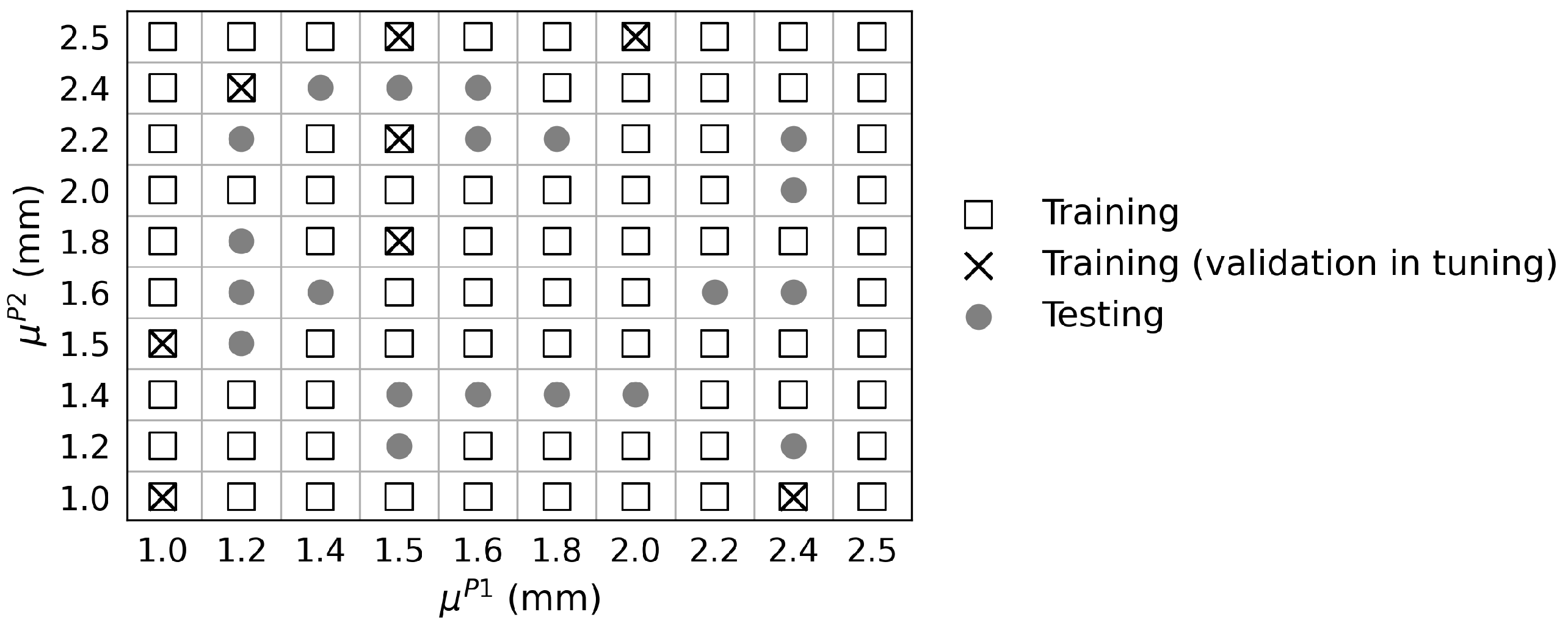
This section presents the surrogate model referred to as ${\mathcal{H}}_3$ for the prediction of the whole displacement profile in the frequency interval of [5,100] Hz. This task is much more difficult than the previous ones, as the output quantity has a dimension of 96, containing much more information to be learned by the model. Therefore, the training set size has been increased to 80 as presented in Figure 12. The model is further evaluated at the remaining 20 samples.

4.3.1. Fully-Connected Network Structure

First, we still adopt a standard neural network with a fully connected structure for the construction of model ${\mathcal{H}}_3$. Compared to model ${\mathcal{H}}_2$, the only difference is that now the output dimension is increased to 96.

Tuning tests are conducted to fix three hyperparameters, and an early-stop scheme helps to save the best model during the training process under each hyperparameter setup. Results are summarized in

Table 4. Error comparison of different networks in model ${\mathcal{H}}_3$ tuning tests. The network 2 (in red) is the final choice.

No.	Dimension Multiplication Factor k	Number of Hidden Layers d	Hidden Layer Dimension D	Trainable Parameters	Training $\mathit{ϵ}$	Validation $\mathit{ϵ}$
1	10	4	50	22,716	2.037%	2.792%
2	10	4	200	175,716	1.835%	2.745%
3	10	4	300	352,716	1.574%	2.855%
4	10	3	250	193,966	1.467%	2.889%
5	20	4	180	179,736	1.315%	3.167%

with the normalized RMSE in Equation (3) as an error indicator. This error is calculated at 8 samples selected from the training set, which are not used for training in tuning tests. As proved, increasing the hidden layer dimension could raise the risk of overfitting. Comparing networks No. 3, No. 4 and No. 5, the model appears to perform better with a deeper structure than wider layers of $L_1$ and $L_{2,d}$ where hyperparameters k and D are larger. Network No. 2 is finally chosen for the surrogate model construction.

The network with selected hyperparameters is trained for 5000 epochs with a batch size of 80. The optimization algorithm is Adam with a constant learning rate of ${10}^{-4}$ and $L2$ regularization of ${10}^{-4}$ is also applied. Figure 13 shows the prediction performance of all 20 samples in the testing set. The surrogate model provides close predictions of the whole displacement profiles on these unseen data. The worst case is noted in the third row and the last column, with normalized RMSE equal to 3.702%. For most samples, the model accurately captures the profile shape, and this suggests that the model has effectively learned a generalized relation between the functional parameters and the displacement outputs. Meanwhile, it presents a visible underestimation of the peak values, and predictions seem to be less satisfying at the natural frequencies’ neighborhood presented in the displacement profiles. The average normalized RMSE for all testing data is 2.153%.

4.3.2. Integrated Network Structure

It has been demonstrated that the approach with a conventional fully connected network structure already provides close approximations of the displacement curves. However, noticeable errors can be observed at the natural frequencies’ neighborhood where the model seems to underestimate these amplitude values. Given the satisfying performance of surrogate models, ${\mathcal{H}}_1$ and ${\mathcal{H}}_2$, here we propose a novel approach with an integrated network structure to enrich the existing model ${\mathcal{H}}_3$ with information from models ${\mathcal{H}}_1$ and ${\mathcal{H}}_2$ in order to improve the prediction accuracy in those regions. To differentiate from the surrogate model ${\mathcal{H}}_3$ with full-connected structure, the new model with the integrated structure will be noted as ${\mathcal{H}}_3^I$.

The integrated structure is illustrated in Figure 14 and emphasizes the fact that the model receives information from previous models ${\mathcal{H}}_1$ and ${\mathcal{H}}_2$: the predicted eigenfrequencies given by model ${\mathcal{H}}_1$ inform the peaks’ locations in the output vector of dimension 96, whereas amplitudes at those eigenfrequencies predicted by ${\mathcal{H}}_2$ enforce the prediction for peak values.

Regarding the network implementation, there are three details to mention:

• Predictions of eigenfrequencies from model ${\mathcal{H}}_1$ are float numbers, and they are rounded to the nearest integer, as they serve further as vector indexes.
• Amplitudes given by ${\mathcal{H}}_2$ are actually the values at the exact natural frequencies ${\mathbf{\omega }}^{{\mathbf{P}}_{\mathbf{1}}+{\mathbf{P}}_{\mathbf{2}}}$ while the displacement amplitudes to be predicted by ${\mathcal{H}}_3^I$ are values at discrete frequencies f within the range of [5, 100] Hz with a step of 1 Hz. Therefore, the predictions from ${\mathcal{H}}_2$ cannot directly replace the values in the output vector. Here, the network must learn the interpolation coefficients in vector $\mathbf{\beta }$ for representing ${\mathbf{u}}_{\mathbf{z}}\left({\mathbf{\omega }}^{{\mathbf{P}}_{\mathbf{1}}+{\mathbf{P}}_{\mathbf{2}}}\right)$ in the prediction of ${\mathbf{u}}_{\mathbf{z}}\left(f\right)$. The final model output ${{\widehat{\mathbf{u}}}_{\mathbf{z}}}^{\prime }\left(f\right)$ under the integrated structure is defined in Equation (4) that is later passed to calculate the loss for back-propagation:

  $${\widehat{\mathbf{u}}}_{\mathbf{z}}^{\prime }\left(f\right)={\widehat{\mathbf{u}}}_{\mathbf{z}}\left(f\right)+\mathbf{\beta }({\mathbf{u}}_{\mathbf{z}}^{\prime }\left(f\right)-{\widehat{\mathbf{u}}}_{\mathbf{z}}\left(f\right))$$

  (4)
• The amplitude predictions given by model ${\mathcal{H}}_2$ are passed to the same scalar for the normalization of output values, used in the pre-processing step before the ${\mathcal{H}}_3$ model training.

The final model ${\mathcal{H}}_3^I$ keeps the same structure of ${\mathcal{H}}_3$ with three hyperparameters $k=10,d=4,D=200$ together with the integration of predictions from ${\mathcal{H}}_1$ and ${\mathcal{H}}_2$. The network is trained for a maximum of 5000 epochs with a batch size of 80. The optimization algorithm is Adam with a constant learning rate of ${10}^{-4}$, and $L2$ regularization of ${10}^{-5}$ is applied.

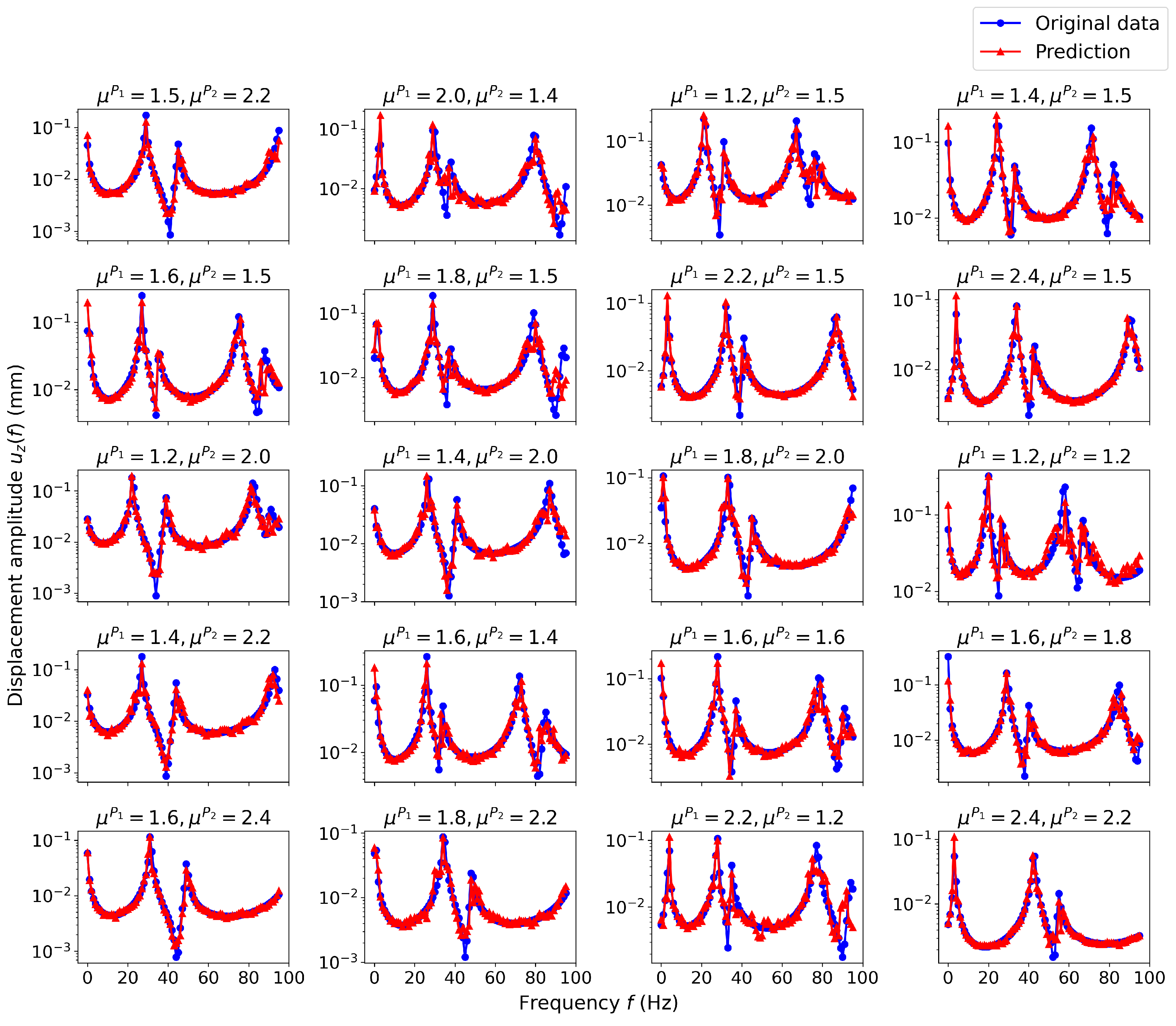
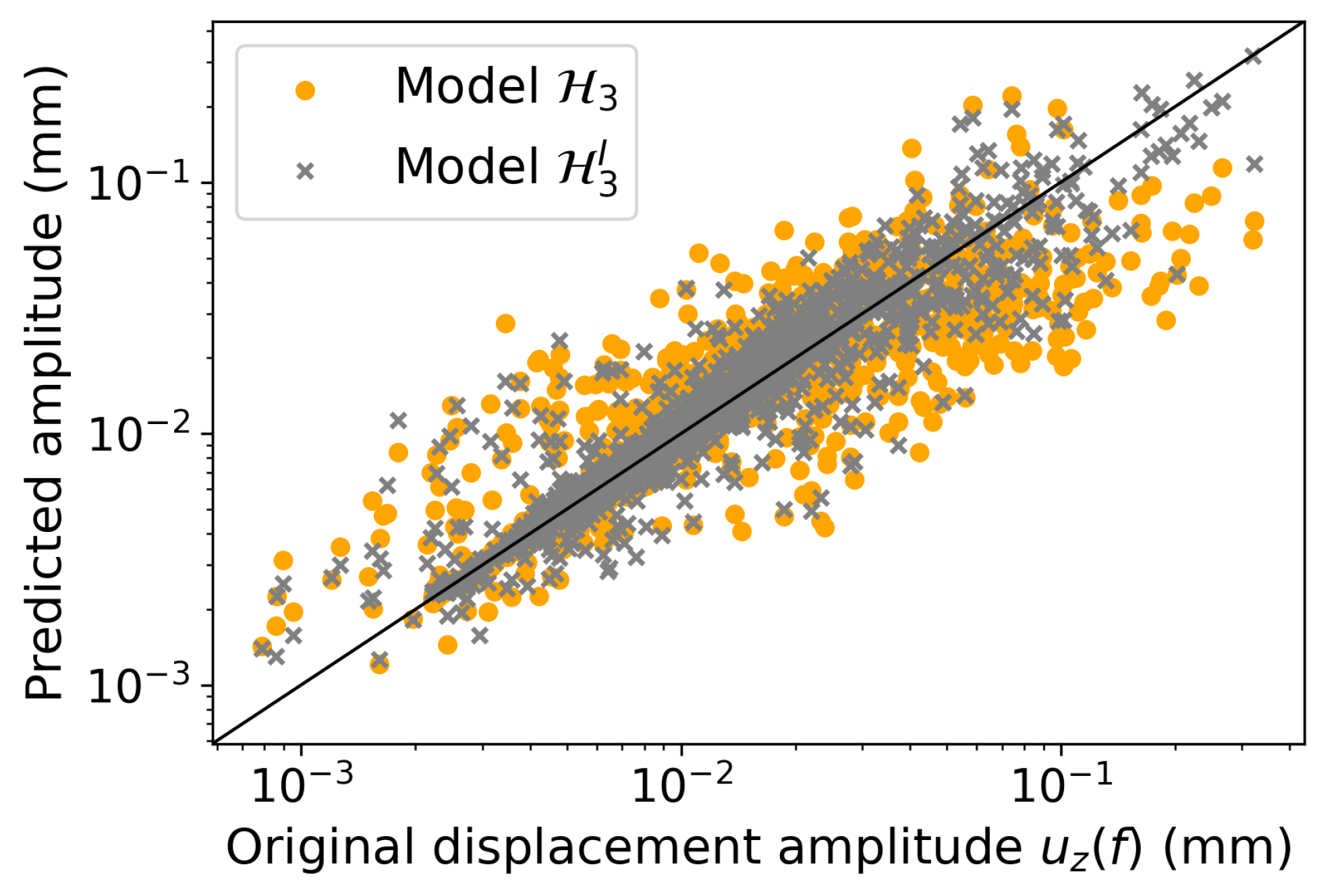
The results of the predicted displacement values and the reference ones are shown in Figure 15, in which each point represents one element value in the displacement profile vector for each of the samples in the testing set. Compared to model ${\mathcal{H}}_3$, it can be observed that the new model with an integrated network structure produces an improvement for large values, which usually corresponds to peak amplitudes in the displacement profile. Respective predictions for the same 20 samples of the testing set are shown in Figure 16. Improvements for peak amplitude predictions are quite visible for all samples, and the total normalized RMSE is reduced from $2.153\%$ to $1.685\%$ with this new approach.

5. Conclusions and Perspectives

In this paper, surrogate modeling based on neural networks is developed for the prediction of assembled system behavior with modal information of the structural components as inputs. The approach is illustrated on an elasto-dynamic problem of a two-component plate. The study starts with a database of 100 configurations, obtained by numerical simulations. For each prediction, only a subset of configuration samples is used as training set, and the model performance is evaluated on unseen data composing the testing set. Tuning experiments are conducted for each model to choose the best network hyperparameters. It is shown that the accuracy of neural networks is remarkable for the prediction of system eigenfrequencies and peak z-component displacement amplitudes at these natural frequencies. The prediction for nodal displacement profile within [5, 100] Hz appears to be much more difficult, considering the variations of configurations in the DOE. The first approach with a fully connected network structure allows capturing the global curve shape while exhibiting some underestimations of large amplitudes. A second network approach with the integration of the previous two models effectively improves the predictions in peak amplitudes and turns out to provide accurate results on unseen data.

From an application perspective, the work in this article can be extended to industrial problems, for example vibro-acoustic studies of a vehicle composed of several structural parts. It would be interesting to adopt surrogate modeling with functional parameters in a project process and evaluate its potential, typically for early stage optimization. These topics constitute a work in progress.