Numerical Analysis of Deformation Characteristics of Elastic Inhomogeneous Rotational Shells at Arbitrary Displacements and Rotation Angles

Abstract

Adequate mathematical models and computational algorithms are developed in this study to investigate specific features of the deformation processes of elastic rotational shells at large displacements and arbitrary rotation angles of the normal line. A finite difference method (FDM) is used to discretize the original continuum problem in spatial variables, replacing the differential operators with a second-order finite difference approximation. The computational algorithm for solving the nonlinear boundary value problem is based on a quasi-dynamic form of the ascertainment method with the construction of an explicit two-layer time-difference scheme of second-order accuracy. The influence of physical and mechanical characteristics of isotropic and composite materials on the deformation features of elastic spherical shells under the action of surface loading of “tracking” type is investigated. The results of the studies conducted have shown that the physical and mechanical characteristics of isotropic and composite materials significantly affect the nature of the deformation of the clamped spherical shell in both the subcritical and post-critical domains. The developed mathematical models and computational algorithms can be applied in the future to study shells of rotation made of hyperelastic (non-linearly elastic) materials and soft shells.

1. Introduction

There are many papers devoted to the study of shells, but there are still a number of unresolved issues that require attention [1,2,3]. Elastic single and multi-layered shells of rotation under the action of an axisymmetric system of boundary or surface static loads of general or local nature are considered. For a single-layer structure, the mid-surface of the shell is taken as the coordinate surface (datum surface); for a multi-layer structure, the mid-surface of one of the layers or the contact surface of the layers can be taken as the coordinate surface. To describe the deformation processes of elastic rotational shells at large displacements of coordinate surface points and unlimited rotation angles of the normal to it, the changes of Cartesian coordinates x, y are taken as unknowns, which allows for the considered variant of geometrically nonlinear deformation of thin-walled constructions to greatly simplify the structure of initial differential equations in comparison with using traditional components of tangential u and normal w displacements [4,5].

Unlike most traditional mathematical models for the study of shell deformation processes, when the geometric parameters of the shell are identical both in the initial and deformed state (for example, the curvature and the parameters of the Lamet before and after deformation are the same), this work takes into account the difference in the geometry of the shell in the initial and final (after loading—genia) state. This makes it possible to study the features of deformation of elastic multi-layer shells in the region of large displacements and angles of rotation of the normal. The developed mathematical models and computational algorithms can be practically implemented in various fields of science and technology, for example, in aerospace systems (deployable elastic antennas, displacement elements of fuel systems) and in the automotive industry when designing automotive-mobile springs made of multi-layer composites, which undergo significant shape changes during operation, etc. These issues are partially considered in the works [6,7].

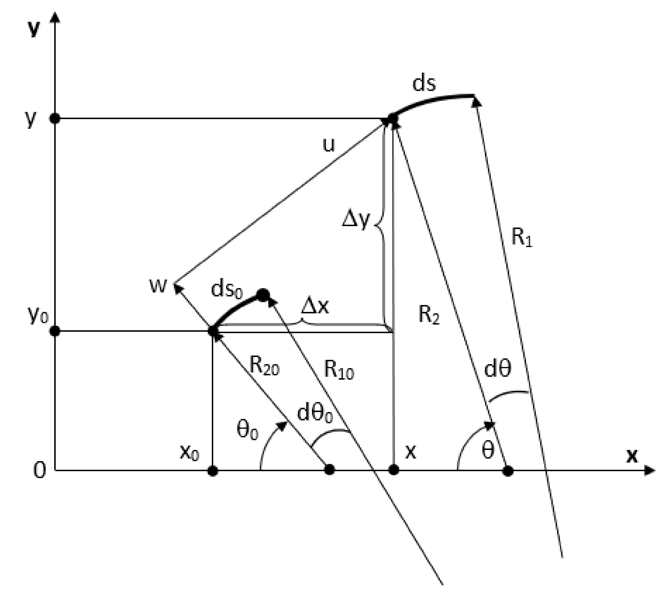
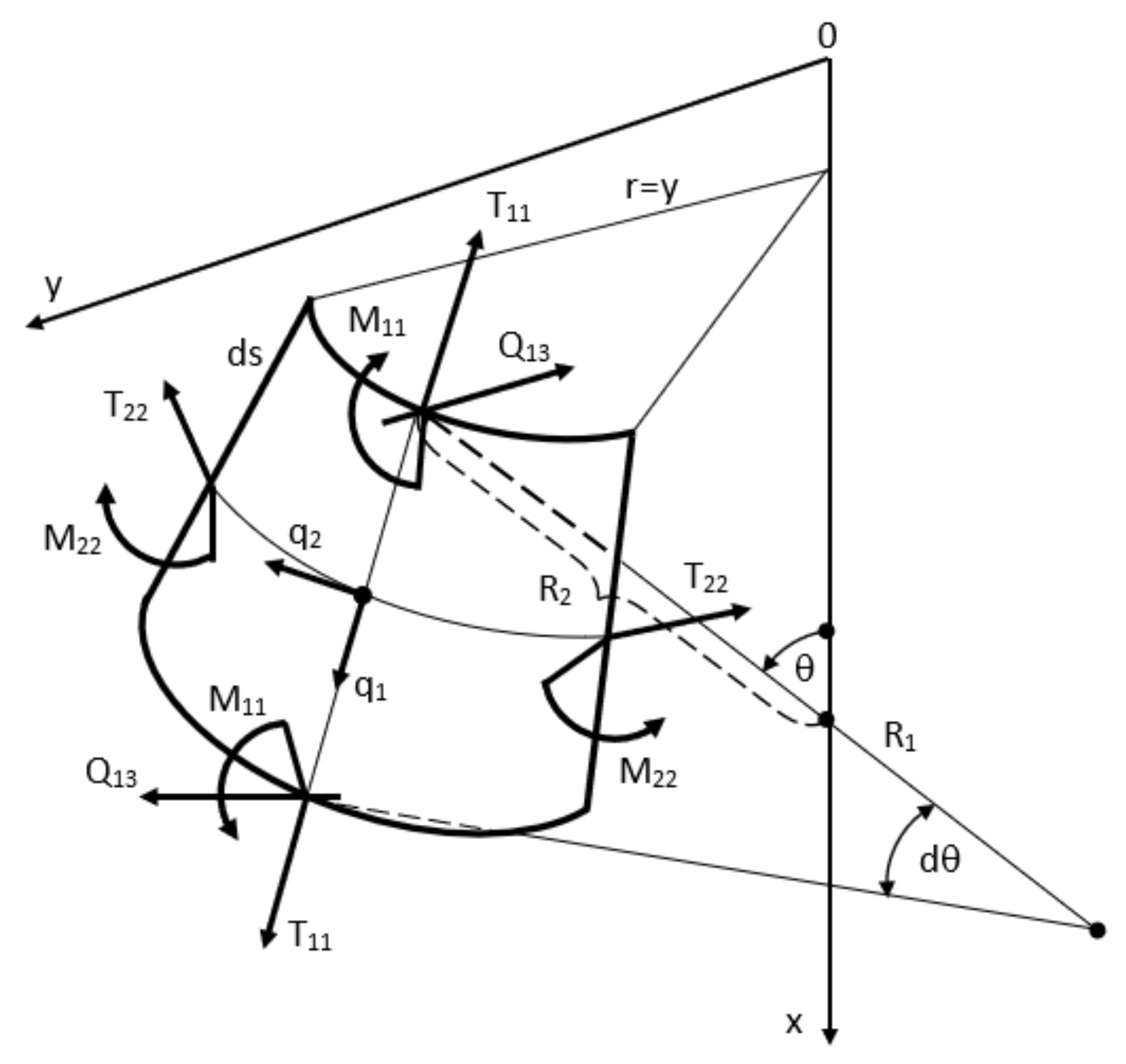
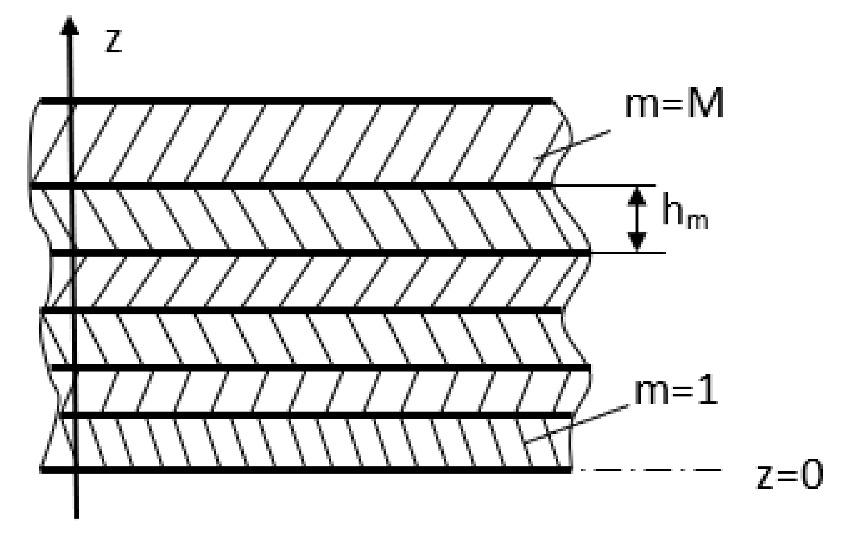
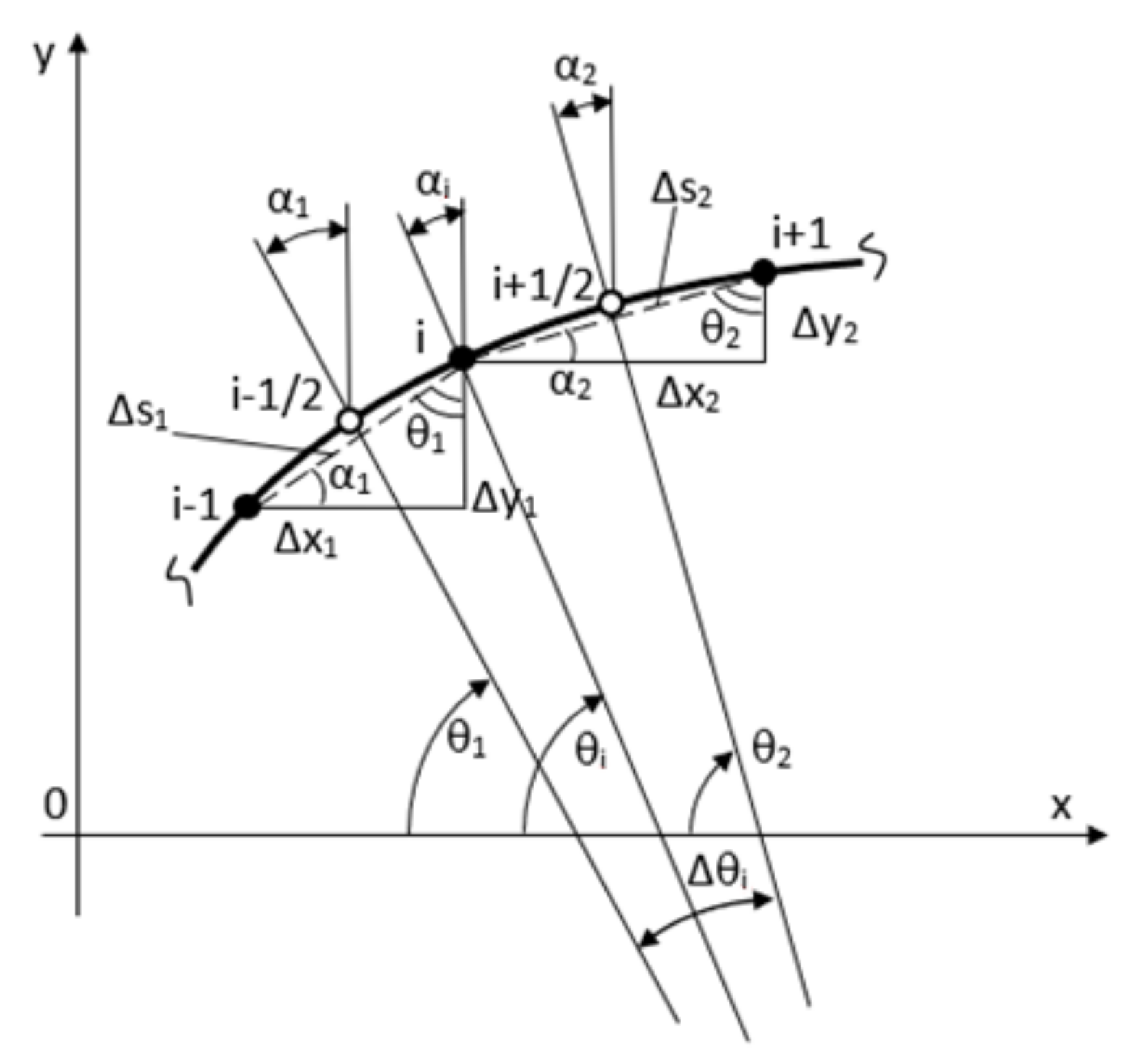
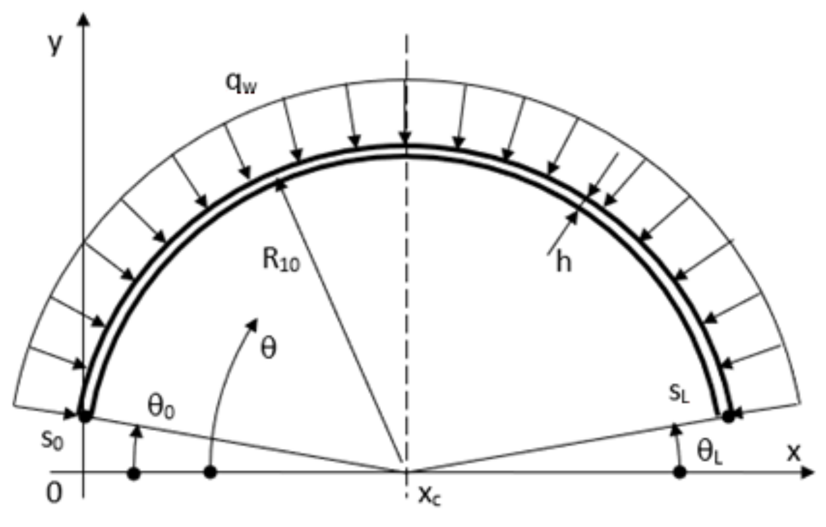
2. Materials and Methods

Before the deformation, an element of an unstrained formative shell of length ds₀ has initial coordinates x₀, y₀, curvatures k₁₀, k_20, and initial angle θ₀ between the x-axis and the normal to the generatrix (Figure 1). Given the coordinates x₀, y₀ as linear coordinate functions along the generatrix x₀ = x₀(s₀), y₀ = y₀(s₀), for the initial (undeformed) state, the following relations take place (1):

$$\begin{gathered} d{s}_0=\sqrt{d{x}_0^2+d{y}_0^2}; \sin {\theta }_0=\frac{d{x}_0}{d{s}_0}; \cos {\theta }_0=\frac{d{y}_0}{d{s}_0}; \\ d{s}_0=R_{10}\cdot d{\theta }_0; k_{10}=\frac{1}{R_{10}}=\frac{d{\theta }_0}{d{s}_0}; k_{20}=\frac{1}{R_{20}}=\frac{\sin {\theta }_0}{y_0}, \end{gathered}$$

(1)

where R₁₀ is the initial radius of curvature of the surface in the direction of the formant; R₂₀ is the initial radius of curvature in the circumferential direction (Figure 1).

After deformation, the element will have length ds, coordinates x, y, and curvatures k₁, k₂. Considering the coordinates x, y as functions of the linear coordinate s along the deformed generatrix x = x(s), y = y(s), it is possible to write down relations similar to (1) for the deformed state (2):

$$\begin{gathered} ds=\sqrt{d{x}^2+d{y}^2};\sin \theta =\frac{dx}{ds};\cos \theta =\frac{dy}{ds}; \\ ds=R_1\cdot d\theta ;k_1=\frac{1}{R_1}=\frac{d\theta }{ds};k_2=\frac{1}{R_2}=\frac{\sin \theta }{y}, \end{gathered}$$

(2)

where $\theta$ is the rotation angle between the normal to the deformed coordinate surface and the x-axis.

There are no restrictions imposed on rotation angles Δθ = θ − θ₀. The deformation components along the generatrix E₁₁ and in the circumferential direction E₂₂ are defined as (3):

$$E_{11}=\frac{ds-d{s}_0}{d{s}_0}=\frac{ds}{d{s}_0}-1;E_{22}=\frac{\pi ·y-\pi ·y_0}{\pi ·y_0}=\frac{y}{y_0}-1.$$

(3)

The curvature change parameters along the generatrix K₁₁ and in the circumferential direction K₂₂ are determined from the obvious ratios (4):

$$K_{11}=k_1-k_{10}=\frac{d\theta }{ds}-\frac{d{\theta }_0}{d{s}_0};K_{22}=k_2-k_{20}=\frac{\sin \theta }{y}-\frac{\sin {\theta }_0}{y_0}.$$

(4)

The deformation components at distance z from the coordinate surface, taking into account the hypotheses and assumptions made for thin shells, are distributed according to a linear law (5):

$$E_{11}^z=E_{11}+z·K_{11};E_{22}^z=E_{22}+z·K_{22}.$$

(5)

We introduce force factors in the cross-section of the shell: longitudinal force T₁₁ and circumferential force T₂₂, transverse force Q₁₃, as well as bending moments M₁₁ and M₂₂: M₁₁—in longitudinal direction, M₂₂—in circumferential direction. A distributed load q = q(s) with components: q₁ = q₁(s) and q₂ = q₂(s) acts on the shell locally or over the entire surface. For the conservative load case q₁ = q_x(s), q₂ = q_y(s), and for the “tracking” load case q₁ = q_u(s), q₂ = q_w(s). The positive directions for the force factors T₁₁, T₂₂, Q₁₃, M₁₁, M₂₂ and load components q₁, q₂ are shown in Figure 2.

In the case of a single-layer construction of an orthotropic material, the forces and moments in the elastic shell are expressed in terms of the deformed state components according to the following dependencies (6), (7) [2,3]:

$$\begin{gathered} T_{11}=B_{11}{E}_{11}+B_{12}{E}_{22};M_{11}=D_{11}{K}_{11}+D_{12}{K}_{22}; \\ {T}_{22}=B_{22}{E}_{22}+B_{21}{E}_{11};M_{22}=D_{22}{K}_{22}+D_{21}{K}_{11}, \end{gathered}$$

(6)

where

$$\begin{gathered} B_{11}=\frac{E_{1}h}{1-{\nu }_{12}{\nu }_{21}};B_{22}=\frac{E_{2}h}{1-{\nu }_{12}{\nu }_{21}};B_{12}={\nu }_{12}{B}_{11};B_{21}={\nu }_{21}{B}_{22}; \\ {D}_{11}=\frac{E_1{h}^3}{12\left(1-{\nu }_{12}{\nu }_{21}\right)};D_{22}=\frac{E_2{h}^3}{12\left(1-{\nu }_{12}{\nu }_{21}\right)};D_{12}={\nu }_{12}{D}_{11};D_{21}={\nu }_{21}{D}_{22}, \end{gathered}$$

(7)

where E₁, E₂ are the Young’s moduli in the longitudinal and circumferential directions, respectively; ν₁₂, ν₂₁ are the Poisson’s ratios: the first index indicates the direction of deformation and the second index indicates the direction of force.

The following correlation between the elastic characteristics of the material takes place (8):

$$E_1{\nu }_{12}=E_2{\nu }_{21}.$$

(8)

For a multi-layer structure as a whole, the conditions of rigid contact between layers without mutual separation and slippage are assumed, whereby layers of variable thickness h_m are generally considered; m is the layer index: 1 ≤ m ≤ M, M is the number of layers (Figure 3).

The force factors in the multi-layer package are expressed in terms of the deformation components of the coordinate surface according to the Formulas (9), (10) [8]:

$$\begin{gathered} T_{11}=B_{11}{E}_{11}+B_{12}{E}_{22}+A_{11}{K}_{11}+A_{12}{K}_{22}; \\ {T}_{22}=B_{21}{E}_{11}+B_{22}{E}_{22}+A_{21}{K}_{11}+A_{22}{K}_{22}; \\ {M}_{11}=A_{11}{E}_{11}+A_{12}{E}_{22}+D_{11}{K}_{11}+D_{12}{K}_{22}; \\ {M}_{22}=A_{21}{E}_{11}+A_{22}{E}_{22}+D_{21}{K}_{11}+D_{22}{K}_{22}, \end{gathered}$$

(9)

where

$$\begin{gathered} B_{11}=\stackrel{\underset{M}{m=1}}{\Sigma }\frac{E_1^{\left(m\right)}}{\left[1-{\nu }_{12}^{\left(m\right)}·{\nu }_{21}^{\left(m\right)}\right]}\left(z_m-z_{m-1}\right);B_{12}=\stackrel{\underset{M}{m=1}}{\Sigma }\frac{E_1^{\left(m\right)}·{\nu }_{12}^{\left(m\right)}}{\left[1-{\nu }_{12}^{\left(m\right)}·{\nu }_{21}^{\left(m\right)}\right]}\left(z_m-z_{m-1}\right); \\ {B}_{22}=\stackrel{\underset{M}{m=1}}{\Sigma }\frac{E_2^{\left(m\right)}}{\left[1-{\nu }_{12}^{\left(m\right)}·{\nu }_{21}^{\left(m\right)}\right]}\left(z_m-z_{m-1}\right);B_{21}=B_{12}; \\ {A}_{11}=\frac{1}{2}·\stackrel{\underset{M}{m=1}}{\Sigma }\frac{E_1^{\left(m\right)}}{\left[1-{\nu }_{12}^{\left(m\right)}·{\nu }_{21}^{\left(m\right)}\right]}\left(z_m^2-z_{m-1}^2\right);A_{12}=\frac{1}{2}·\stackrel{\underset{M}{m=1}}{\Sigma }\frac{E_1^{\left(m\right)}·{\nu }_{12}^{\left(m\right)}}{\left[1-{\nu }_{12}^{\left(m\right)}·{\nu }_{21}^{\left(m\right)}\right]}\left(z_m^2-z_{m-1}^2\right); \\ {A}_{22}=\frac{1}{2}·\stackrel{\underset{M}{m=1}}{\Sigma }\frac{E_2^{\left(m\right)}}{\left[1-{\nu }_{12}^{\left(m\right)}·{\nu }_{21}^{\left(m\right)}\right]}\left(z_m^2-z_{m-1}^2\right);A_{21}=A_{12}; \\ {D}_{11}=\frac{1}{3}·\stackrel{\underset{M}{m=1}}{\Sigma }\frac{E_1^{\left(m\right)}}{\left[1-{\nu }_{12}^{\left(m\right)}·{\nu }_{21}^{\left(m\right)}\right]}\left(z_m^3-z_{m-1}^3\right);D_{12}=\frac{1}{3}·\stackrel{\underset{M}{m=1}}{\Sigma }\frac{E_1^{\left(m\right)}·{\nu }_{12}^{\left(m\right)}}{\left[1-{\nu }_{12}^{\left(m\right)}·{\nu }_{21}^{\left(m\right)}\right]}\left(z_m^3-z_{m-1}^3\right); \\ {D}_{22}=\frac{1}{3}·\stackrel{\underset{M}{m=1}}{\Sigma }\frac{E_2^{\left(m\right)}}{\left[1-{\nu }_{12}^{\left(m\right)}·{\nu }_{21}^{\left(m\right)}\right]}\left(z_m^3-z_{m-1}^3\right);D_{21}=D_{12}. \end{gathered}$$

(10)

Formula (10) is obtained by assuming the constancy of the elastic characteristics of the material $E_1^{\left(m\right)},{\nu }_{12}^{\left(m\right)},E_2^{\left(m\right)},{\nu }_{21}^{\left(m\right)}$ within the m-layer [9,10,11]. The equilibrium equations of the deformed element of a rotational shell have the following form (11) [4,5,8]:

$$\begin{gathered} \frac{1}{y}\frac{d}{ds}\left(y·T_{11}\right)-\frac{\cos \theta }{y}·T_{22}+k_1·Q_{13}+q_1=0; \\ \frac{1}{y}\frac{d}{ds}\left(y·Q_{13}\right)-k_1·T_{11}-k_2·T_{22}+q_2=0; \\ {Q}_{13}=\frac{1}{y}\frac{d}{ds}\left(y·M_{11}\right)-\frac{\cos \theta }{y}·M_{22}. \end{gathered}$$

(11)

The system of differential equations of the developed mathematical model (1)–(11) is supplemented by boundary conditions at the edges s = s₀ and s = s_L. The characteristic boundary conditions at the edge s = s₀ can be written in the following way:

• rigid fixing (12):

$$\begin{gathered} x\left(s_0\right)=x_0; \\ y\left(s_0\right)=y_0; \\ \theta \left(s_0\right)={\theta }_0; \end{gathered}$$

(12)

• pin-edge fixing (13):

$$\begin{gathered} x\left(s_0\right)=x_0; \\ y\left(s_0\right)=y_0; \\ {M}_{11}\left(s_0\right)=0. \end{gathered}$$

(13)

The boundary conditions at the edge s = s_L are formulated similarly to (12)–(13).

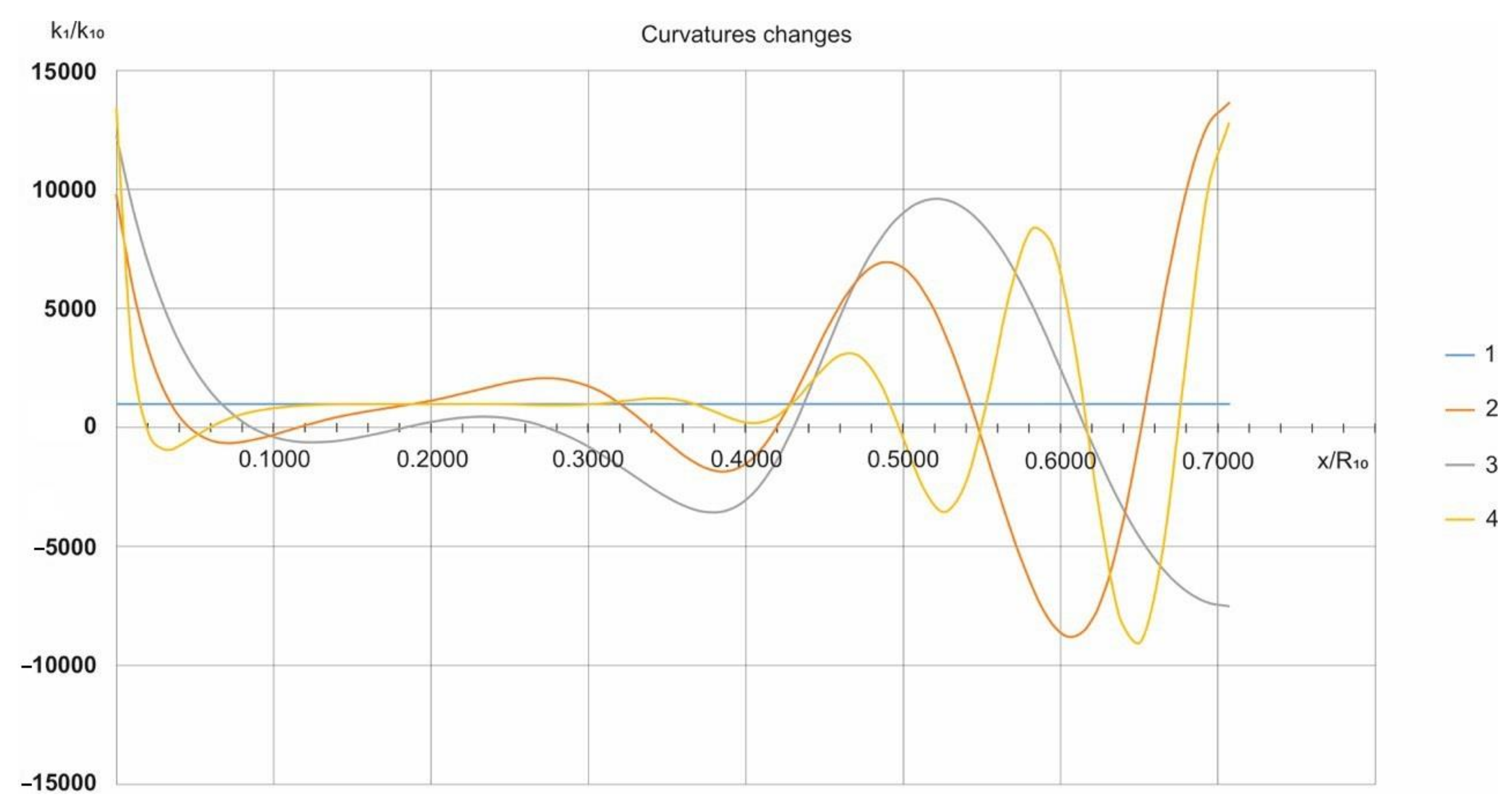
3. Results and Discussion

When constructing the discrete analog of the original continuum problem (1)–(13), FDM [3,4] is used to discretize the spatial variables. Two grids are introduced in the area of continuous variation of the argument s: a main grid with integer indices i and an auxiliary grid with indices i ± 1/2, the nodes of which are positioned in the middle between the nodes of the main grid i ± 1 (Figure 4).

The partial derivatives in differential relations (1)–(13) are approximated by difference operators of second-order accuracy (Δs²). The undeformed state of the shell is given by the grid functions (x₀)_i, (y₀)_i. Stress-strain state (SSS) parameters (1)–(10) are related to main and auxiliary grid nodes. Finite-difference approximations of differential relations (1) for the initial state of the rotational shell can be represented in the following way (14), (15):

$$\begin{gathered} {(\Delta s_0)}_{i-1/2}=\Delta s_1=\sqrt{\Delta x_1^2+\Delta y_1^2};{(\Delta s_0)}_{i+1/2}=\Delta s_2=\sqrt{\Delta x_2^2+\Delta y_2^2}; \\ \sin {\alpha }_1=\frac{\Delta y_1}{\Delta s_1};{\theta }_1={({\theta }_0)}_{i-1/2}=\frac{\pi }{2}-{\alpha }_1; \\ \sin {\alpha }_2=\frac{\Delta y_2}{\Delta s_2};{\theta }_2={({\theta }_0)}_{i+1/2}=\frac{\pi }{2}-{\alpha }_2; \\ {(\Delta s_0)}_i=\frac{{(\Delta s_0)}_{i-1/2}+{(\Delta s_0)}_{i+1/2}}{2};{(k_{10})}_i=\frac{{({\theta }_0)}_{i+1/2}-{({\theta }_0)}_{i-1/2}}{{(\Delta s_0)}_i}, \end{gathered}$$

(14)

where

$$\begin{gathered} \Delta x_1={(x_0)}_i-{(x_0)}_{i-1};\Delta y_1={(y_0)}_i-{(y_0)}_{i-1}; \\ \Delta x_2={(x_0)}_{i+1}-{(x_0)}_i;\Delta y_2={(y_0)}_{i+1}-{(y_0)}_i. \end{gathered}$$

(15)

In the relations (14), (15) the grid functions (x₀)_i, (y₀)_i are set from the condition of constancy of the step Δs₀ = const for the whole computational domain of the shell 0 ≤ s₀ ≤ L₀, so (16):

$$\Delta s_0=\frac{L_0}{N-1};\Delta s={(\Delta s_0)}_{i-1/2}={(\Delta s_0)}_{i+1/2},$$

(16)

where N is the number of sampling points: 1 ≤ i ≤ N.

The deformed state parameters of the shell are described by the grid functions of nodal displacements x_i and y_i with approximation of relations (2) by finite difference operators (17), (18) similar to (14), (15) (Figure 4):

$$\begin{gathered} \Delta s_{i-1/2}=\Delta s_1=\sqrt{\Delta x_1^2+\Delta y_1^2};\Delta s_{i+1/2}=\Delta s_2=\sqrt{\Delta x_2^2+\Delta y_2^2}; \\ \sin {\alpha }_1=\frac{\Delta y_1}{\Delta s_1};\sin {\alpha }_2=\frac{\Delta y_2}{\Delta s_2};{\theta }_1={\theta }_{i-1/2}=\frac{\pi }{2}-{\alpha }_1;{\theta }_2={\theta }_{i+1/2}=\frac{\pi }{2}-{\alpha }_2; \\ \Delta s_i=\frac{\Delta s_{i-1/2}+\Delta s_{i+1/2}}{2};{(k_1)}_i=\frac{{\theta }_{i+\frac{1}{2}}-{\theta }_{i-\frac{1}{2}}}{\Delta s_i}, \end{gathered}$$

(17)

where

$$\begin{gathered} \Delta x_1=x_i-x_{i-1};\Delta y_1=y_i-y_{i-1}; \\ \Delta x_2=x_{i+1}-x_i;\Delta y_2=y_{i+1}-y_i. \end{gathered}$$

(18)

The grid functions of the strain and curvature change components in (3) and (4) are approximated at the corresponding nodes of the main and auxiliary grid as follows (19):

$$\begin{gathered} {(E_{11})}_{i\pm 1/2}=\frac{\Delta s_{i\pm 1/2}-{(\Delta s_0)}_{i\pm 1/2}}{{(\Delta s_0)}_{i\pm 1/2}};{(E_{22})}_i=\frac{y_i}{{(y_0)}_i}-1; \\ {(K_{11})}_i={(k_1)}_i-{(k_{10})}_i;{(K_{22})}_{i\pm 1/2}={(k_2)}_{i\pm 1/2}-{(k_{20})}_{i\pm 1/2}. \end{gathered}$$

(19)

As follows from relations (14)–(18), uniform finite-difference approximations are used to describe both the initial state and the deformed state [1,2]. The finite-difference analogs of equilibrium equations (11), discretized with respect to the node point of the main grid i, are written in the following form (20), (21):

$$\begin{gathered} \frac{1}{y_i}\frac{{(y·T_{11})}_{i+1/2}-{(y·T_{11})}_{i-1/2}}{\Delta s_i}-{\left(\frac{\cos \theta }{y}·T_{22}\right)}_i+{(k_1)}_i·\frac{{(Q_{13})}_{i-1/2}+{(Q_{13})}_{i+1/2}}{2}+{(q_1)}_i=0; \\ \frac{1}{y_i}\frac{{(y·Q_{13})}_{i+1/2}-{(y·Q_{13})}_{i-1/2}}{\Delta s_i}-{(k_1)}_i·\frac{{(T_{11})}_{i-1/2}+{(T_{11})}_{i+1/2}}{2}-{\left(k_2·T_{22}\right)}_i+{(q_2)}_i=0, \end{gathered}$$

(20)

where

$$\begin{gathered} {\left(Q_{13}\right)}_{i-1/2}=\frac{1}{y_{i-1/2}}\frac{{(y·M_{11})}_i-{(y·M_{11})}_{i-1}}{\Delta s_{i-1/2}}-{\left(\frac{\cos \theta }{y}·M_{22}\right)}_{i-1/2}; \\ {\left(Q_{13}\right)}_{i+1/2}=\frac{1}{y_{i+1/2}}\frac{{(y·M_{11})}_{i+1}-{(y·M_{11})}_i}{\Delta s_{i+1/2}}-{\left(\frac{\cos \theta }{y}·M_{22}\right)}_{i+1/2}, \end{gathered}$$

(21)

where (q₁)_i, (q₂)_i are the grid functions of the surface loading components.

Since for approximation of VAT parameters in initial and deformed states the same type finite-difference approximations (14)–(19) are used, then at (q₁)_i = (q₂)_i = 0 the non-deformed state given by relations (14), (15) is the exact solution of grid equations (20), that confirms the correctness of developed difference approximations (14)–(21). To construct a computational algorithm for solving the system of nonlinear grid equations (20), a quasi-dynamic form of the establishment method is used [3,4,5,9]. To construct the evolutionary problem, the grid analogs of equilibrium equations (20) are replaced by non-stationary equations that have the same form as the shell’s equations of motion in a viscous medium [1,2,3,5]. The finite-difference analogs of the equilibrium equations (20) in operator form are represented as (22):

$${[L_{\Delta s}\left(U_k\right)]}_i+{(q_k)}_i=0,$$

(22)

where ${[L_{\Delta s}\left(U_k\right)]}_i$ are the corresponding generalised finite-difference operators for the vector U_k of the grid displacement functions; (k = 1, 2).

For the case of “tracking” load, to simplify the computational procedure, it is advisable to build an iterative process with respect to the displacements of the local basis u, w, followed by recalculation in the x, y coordinate system (Figure 1). Then the non-stationary setting method equations for the node point of the main grid will be written in the following way (23):

$${[L_{\Delta s}\left(U_k\right)]}_i+{(q_k)}_i={(m_k{\ddot{u}}_k)}_i+{({\epsilon }_k{\dot{u}}_k)}_i,$$

(23)

where m_k = ρh; ρ is the density; (u₁)_i = u_i, (u₂)_i = w_i, (q₁)_i = (q_u)_i, (q₂)_i = (q_w)_i; ε_k is the medium specific viscosity parameters; (k = 1, 2).

The point indicates the differentiation by time t. Approximation of equations (23) on a time grid with step Δt = const using difference operators of second-order accuracy O(Δ $t^2$) makes it possible to obtain explicit expressions for velocities ${\left[{\dot{u}}_k\right]}_i^{\left(n+1/2\right)}$ on time layer t^(n+1/2) and grid functions for the generalized displacements ${\left[u_k\right]}_i^{\left(n+1\right)}$ on time layer t⁽ⁿ⁺¹⁾ (24):

$$\begin{gathered} {\left[{\dot{u}}_k\right]}_i^{\left(n+1/2\right)}=\frac{{\left[{2m}_k-{\epsilon }_k\Delta t\right]}_i}{{\left[{2m}_k+{\epsilon }_k\Delta t\right]}_i}·{\left[{\dot{u}}_k\right]}_i^{\left(n-1/2\right)}+\frac{2\Delta t·{\left[L_{\Delta s}\left(U_k\right){+q}_k\right]}_i^{\left(n\right)}}{{\left[{2m}_k+{\epsilon }_k\Delta t\right]}_i}; \\ {\left[u_k\right]}_i^{\left(n+1\right)}={\left[u_k\right]}_i^{\left(n\right)}+\Delta t·{\left[{\dot{u}}_k\right]}_i^{\left(n+1/2\right)}. \end{gathered}$$

(24)

The grid functions of displacements x_i, y_i of the node points in the x, y coordinate system can be recalculated through the grid functions of the displacement components u_i, w_i in the following way (25), (26) (Figure 1):

$$\begin{gathered} x_i={(x_0)}_i+\Delta x_i; \\ {y}_i={(y_0)}_i+\Delta y_i, \end{gathered}$$

(25)

where

$$\begin{gathered} \Delta x_i=u_i·\sin {({\theta }_0)}_i-w_i·\cos {({\theta }_0)}_i; \\ \Delta y_i=u_i·\cos {({\theta }_0)}_i+w_i·\sin {({\theta }_0)}_i. \end{gathered}$$

(26)

Thus, the difference approximation of the non-stationary equations (23) leads to the iterative process (24) of finding the solution to the original stationary problem (22). The computational algorithm for solving the nonlinear problem in the case of conservative loading is constructed similarly to (23), (24). Iteration process parameters—specific viscosities of the medium ε_k(i) and step in time Δt—are determined from the condition of accelerated convergence and stability of the difference scheme [3,4]. The works related to the study of inhomogeneous elastic shells are reviewed in publications [12,13,14,15,16,17,18,19,20,21,22,23,24,25,26,27,28,29,30,31,32,33,34,35,36,37,38,39,40,41,42,43]. Estimating formulas, taking into account the structure of equations (23), can be written in the form (27) [5,8,9]:

$${\epsilon }_k=2{\mathit{a}}_{\epsilon ,\left(k\right)}\sqrt{\frac{m_k{\mu }_{1,\left(k\right)}{\mu }_{2,\left(k\right)}}{{\mu }_{1,\left(k\right)}+{\mu }_{2,\left(k\right)}};}\Delta t_k=2{\mathit{a}}_{t,\left(k\right)}\sqrt{\frac{m_k}{{\mu }_{1,\left(k\right)}+{\mu }_{2,\left(k\right)}}},$$

(27)

where μ_1(k) and μ_2,(k) are the smallest and largest eigenvalues for the corresponding difference operators in equations (22); a_ε,(k) and a_t,(k) are the correction factors close to unity.

The time step Δt for the whole difference scheme is determined from the condition of the form (28):

$$\Delta t=\underset{k}{min}\Delta t_k.$$

(28)

For nonlinear problems, the exact determination of the boundaries of the difference operator spectra is associated with considerable mathematical difficulties, so μ_1(k) and μ_2(k) are evaluated within the framework of linear relations with appropriate simplifications in the original equations. The evaluation formulas for μ_1(k) and μ_2(k) for the case of a single-layer orthotropic construction can be represented in the following way:

• the smallest eigenvalues (29):

$$\begin{gathered} {\mu }_{1,\left(1\right)}=4\frac{B_{11}}{\Delta s_0^2}·{\sin }^2\frac{\pi }{2}\frac{\Delta s_0}{L_0}; \\ {\mu }_{1,\left(2\right)}=16\frac{D_{11}}{\Delta s_0^4}{\sin }^4\frac{\pi }{2}\frac{\Delta s_0}{L_0}+k_{10}^2{B}_{11}+k_{20}^2{B}_{22}; \end{gathered}$$

(29)

• the largest eigenvalues (30):

$$\begin{gathered} {\mu }_{2,\left(1\right)}=4\frac{B_{11}}{\Delta s_0^2}·{\cos }^2\frac{\pi }{2}\frac{\Delta s_0}{L_0}; \\ {\mu }_{2,\left(2\right)}=16\frac{D_{11}}{\Delta s_0^4}{\cos }^4\frac{\pi }{2}\frac{\Delta s_0}{L_0}+k_{10}^2{B}_{11}+k_{20}^2{B}_{22}, \end{gathered}$$

(30)

where k₁₀, k₂₀ are the characteristic values of the shell curvature parameters.

Based on the developed mathematical models and computational procedures, (1)–(30) there was conducted a study on the influence of physico-mechanical characteristics of isotropic and composite materials on the deformation features of the elastic spherical shell in the subcritical and post-critical regions. A single-layer spherical shell of constant thickness h under the action of a static uniformly distributed external load of the “tracking” type with intensity q_w was considered. Geometric parameters of the shell: R₁₀/h = 200; x_c = 0.707·R₁₀; y_c = 0; θ₀ = θ_L = 15⁰, where R₁₀—the initial radius of curvature (Figure 5). At the edges of the shell s = s₀ and s = s_L the rigid fixing boundary conditions were considered (12).

The intensity of the surface-distributed external pressure q_w was determined through the value of the load parameter p_q in relation to the critical pressure q_cr for a closed isotropic spherical shell with radius R = R₁₀:

The intensity of the surface-distributed external pressure q_w was determined through the value of the load parameter p_q in relation to the critical pressure q_cr for a closed isotropic spherical shell with radius R = R₁₀ (31):

$$q_w=p_q·q_{cr};q_{cr}=\frac{2·E}{\sqrt{3·\left(1-{\nu }^2\right)}}{\left(\frac{h}{R}\right)}^2.$$

(31)

The influence of physical and mechanical characteristics of isotropic and orthotropic materials on peculiarities of nonlinear deformation of the shell in the subcritical and post-critical regions has been investigated. Carbon fiber composite with the following combinations of Young’s moduli E₁ and E₂ in formula (6) [3,5,8] was considered as an orthotropic material (32):

E₁ > E₂: E₁ = 11.25·E₂; ν₂₁ = 0.289;
E₁ < E₂: E₁ = 0.083·E₂; ν₁₂ = 0.289.

(32)

The value of Young’s modulus E of the isotropic material in relation to the moduli E₁ and E₂ of the carbon fiber-reinforced plastic was: E = 0.39·E_max, where E_max = max(E₁, E₂). Poisson’s ratio of an isotropic material: ν = 0.3. The studies were conducted for load parameter values p_q = 0.566; 1.18; 2.36. Due to the symmetry of the problem, the calculation domain was ½ of a shell structure bounded by the parameters: θ₀ ≤ θ ≤ π/2. In the numerical solution of the problem, the number of sampling points 1 ≤ i ≤ N was assumed to be N = 57. The node point with index i = 1 corresponded to the clamped edge of the shell s₀, and at the node point i = 57 at θ = π/2 the conditions of solution symmetry were fulfilled. Figure 6 illustrates the change in k₁/k₁₀ curvatures at p_q = 2.36 for the considered variants of isotropic and orthotropic materials. The horizontal line1 corresponds to the curvature of the spherical shell in the initial (undeformed) state: k₁₀ = const. Curve 2 describes the change in curvature k₁/k₁₀ for an isotropic material (E₁ = E₂), and curves 3 (E₁ > E₂) and 4 (E₁ < E₂)—for an orthotropic material. When building the dependencies in Figure 6, Microsoft Office Excel application was used.

4. Conclusions

The results of the studies conducted have shown that the physical and mechanical characteristics of isotropic and composite materials significantly affect the nature of the deformation of the clamped spherical shell in both the subcritical and post-critical domains. The most optimal variant in terms of increasing the bearing capacity and reducing the deformability of the shell is the carbon fiber reinforced plastic with the Young’s modulus ratio E₂ > E₁. At the same time, maximum displacements u,w in the shell for isotropic material were of order max(u,w) ≈ 5·h at the maximum rotation angles of normal max(Δθ) ≈ 0.15·π, and for orthotropic material maximum values of deformed state parameters were of order max(u,w) ≈ 20·h, max(Δθ) ≈ 0.2·π—for the case E₁ > E₂, and max(u,w) ≈ 2·h, max(Δθ) ≈ 0.07·π—for E₂ > E₁. The results obtained can be applied to the use of additive technologies in the aviation and space industries.

The developed mathematical models and computational algorithms can be applied in the future to study shells of rotation made of hyperelastic (non-linearly elastic) materials and soft shells.

References

1. Babaytsev, A.V.; Rabinskiy, L.N.; Thu Aung, K. Investigation of the contact zone of a cylindrical shell located between two parallel rigid plates with a gap. INCAS Bull. 2020, 12, 43–52. [Google Scholar] [CrossRef]
2. Babaytsev, A.V.; Zotov, A.A. Designing and calculation of extruded sections of an inhomogeneous composition. Russ. Met. 2019, 2019, 1452–1455. [Google Scholar] [CrossRef]
3. Lomakin, E.; Rabinskiy, L.; Radchenko, V.; Solyaev, Y.; Zhavoronok, S.; Babaytsev, A. Analytical estimates of the contact zone area for a pressurized flat-oval cylindrical shell placed between two parallel rigid plates. Meccanica 2018, 53, 3831–3838. [Google Scholar] [CrossRef]
4. Dmitriev, V.G.; Egorova, O.V.; Starovoitov, E.I. Particularities of mathematical modeling of deformation processes for arched and panel designs of composites with large displacements and rotation angles. INCAS Bull. 2020, 12, 53–66. [Google Scholar] [CrossRef]
5. Dmitriev, V.G.; Biryukov, V.I.; Egorova, O.V.; Zhavoronok, S.I.; Rabinskii, L.N. Nonlinear deforming of laminated composite shells of revolution under finite deflections and normal’s rotation angles. Russ. Aeronaut. 2017, 60, 169–176. [Google Scholar] [CrossRef]
6. Grigolyuk, E.I.; Shalashilin, V.I. The method of parameter continuation in problems of nonlinear deformation of rods, plates and shells. Stud. Theory Plat Shells 1984, 17, 3–58. [Google Scholar]
7. Grigolyuk, E.I.; Shalashilin, V.I. Problems of Nonlinear Deformation: A Method for Continuing the Solution by Parameter in Nonlinear Problems of Mechanics of a Solid Deformable Body; Science: Moscow, Russia, 1988. [Google Scholar]
8. Dmitriev, V. Applied mathematics technologies in nonlinear mechanics of thin-walled constructions. In Mathematics Applied to Engineering and Management; Routledge: London, UK, 2019; pp. 71–116. [Google Scholar]
9. Babaytsev, A.V.; Rabinskiy, L.N. Design calculation technique for thick-walled composite constructions operating under high-speed loading. Period. Tche Quim. 2019, 16, 480–489. [Google Scholar] [CrossRef]
10. Bakhvalov, N.S.; Zhidkov, N.P.; Kobelkov, G.M. Numerical Methods; Nauka: Moscow, USSR, 1987. [Google Scholar]
11. Dmitriev, V.G.; Preobrazhensky, I.N. Deformation of flexible shells with cutouts. News USSR Ac. Sci. 1988, 1, 177–184. [Google Scholar]
12. Dmitriev, V.G.; Egorova, O.V.; Zhavoronok, S.I.; Rabinsky, L.N. Investigation of buckling behavior for thin-walled bearing aircraft structural elements with cutouts by means of numerical simulation. Russ. Aer. 2018, 61, 165–174. [Google Scholar] [CrossRef]
13. Babaytsev, A.V.; Orekhov, A.; Rabinskiy, L.N. Properties and microstructure of AlSi10Mg samples obtained by selective laser melting. Nanosci. Technol. Int. J. 2020, 11, 213–222. [Google Scholar] [CrossRef]
14. Dudkin, K.K.; Alifanov, O.M.; Babaitsev, A.V. Determination of the thermophysical characterisitics of the Moon soil with depthed thermoprobes. J. Phys. Conf. Ser. 2020, 1683, 032023. [Google Scholar] [CrossRef]
15. Kyaw, Y.K.; Pronina, P.F.; Polyakov, P.O. Mathematical modelling of the effect of heat fluxes from external sources on the surface of spacecraft. J. Appl. Eng. Sci. 2020, 18, 732–736. [Google Scholar]
16. Astapov, A.N.; Kuznetsova, E.L.; Rabinskiy, L.N. Operating capacity of anti-oxidizing coating in hypersonic flows of air plasma. Surf. Rev. Lett. 2019, 26, 1850145. [Google Scholar] [CrossRef]
17. Egorova, O.V.; Kyaw, Y.K. Solution of inverse non-stationary boundary value problems of diffraction of plane pressure wave on convex surfaces based on analytical solution. J. Appl. Eng. Sci. 2020, 18, 676–680. [Google Scholar] [CrossRef]
18. Zagovorchev, V.A.; Tushavina, O.V. Selection of temperature and power parameters for multi-modular lunar jet penetrator. INCAS Bull. 2019, 11, 231–241. [Google Scholar] [CrossRef]
19. Zagovorchev, V.A.; Tushavina, O.V. The use of jet penetrators for movement in the lunar soil. INCAS Bull. 2019, 11, 121–130. [Google Scholar] [CrossRef]
20. Vahterova, Y.A.; Fedotenkov, G.V. The inverse problem of recovering an unsteady linear load for an elastic rod of finite length. J. Appl. Eng. Sci. 2020, 18, 687–692. [Google Scholar] [CrossRef]
21. Fedotenkov, G.V.; Tarlakovsky, D.V.; Vahterova, Y.A. Identification of non-stationary load upon timoshenko beam. Lobachevskii J. Math. 2019, 40, 439–447. [Google Scholar] [CrossRef]
22. Ivannikov, S.I.; Vahterova, Y.A.; Utkin, Y.A.; Sun, Y. Calculation of strength, rigidity, and stability of the aircraft fuselage frame made of composite materials. INCAS Bull. 2021, 13, 77–86. [Google Scholar] [CrossRef]
23. Vahterova, Y.A.; Min, Y.N. Effect of shape of armoring fibers on strength of composite materials. Turk. J. Comp. Math. Educ. 2021, 12, 2703–2708. [Google Scholar]
24. Starovoitov, E.I.; Zakharchuk, Y.V.; Kuznetsova, E.L. Elastic circular sandwich plate with compressible filler under axially symmetrical thermal force load. J. Balk. Tribol. Assoc. 2021, 27, 175–188. [Google Scholar]
25. Kuznetsova, E.L.; Makarenko, A.V. Mathematical model of energy efficiency of mechatronic modules and power sources for prospective mobile objects. Period. Tche Quim. 2019, 16, 529–541. [Google Scholar] [CrossRef]
26. Bulychev, N.A.; Kuznetsova, E.L. Ultrasonic application of nanostructured coatings on metals. Russ. Eng. Res. 2019, 39, 809–812. [Google Scholar] [CrossRef]
27. Kuznetsova, E.L.; Rabinskiy, L.N. Heat transfer in nonlinear anisotropic growing bodies based on analytical solution. Asia Life Sci. 2019, 2, 837–846. [Google Scholar]
28. Kuznetsova, E.L.; Rabinskiy, L.N. Numerical modeling and software for determining the static and linkage parameters of growing bodies in the process of non-stationary additive heat and mass transfer. Period. Tche Quim. 2019, 16, 472–479. [Google Scholar]
29. Kuznetsova, E.L.; Rabinskiy, L.N. Linearization of radiant heat fluxes in the mathematical modeling of growing bodies by the action of high temperatures in additive manufacturing. Asia Life Sci. 2019, 2, 943–954. [Google Scholar]
30. Babaytsev, A.V.; Kuznetsova, E.L.; Rabinskiy, L.N.; Tushavina, O.V. Investigation of permanent strains in nanomodified composites after molding at elevated temperatures. Period. Tche Quim. 2020, 17, 1055–1067. [Google Scholar] [CrossRef]
31. Rabinsky, L.N.; Kuznetsova, E.L. Simulation of residual thermal stresses in high-porous fibrous silicon nitride ceramics. Powd. Metall. Met. Ceram. 2019, 57, 663–669. [Google Scholar] [CrossRef]
32. Sun, Y.; Kolesnik, S.A.; Kuznetsova, E.L. Mathematical modeling of coupled heat transfer on cooled gas turbine blades. INCAS Bull. 2020, 12, 193–200. [Google Scholar] [CrossRef]
33. Antufev, B.A.; Kuznetsova, E.L.; Rabinskiy, L.N.; Tushavina, O.V. Investigation of a complex stress-strain state of a cylindrical shell with a dynamically collapsing internal elastic base under the influence of temperature fields of various physical nature. Asia Life Sci. 2019, 2, 689–696. [Google Scholar]
34. Antufev, B.A.; Kuznetsova, E.L.; Rabinskiy, L.N.; Tushavina, O.V. Complex stressed deformed state of a cylindrical shell with a dynamically destructive internal elastic base under the action of temperature fields of various physical nature. Asia Life Sci. 2019, 2, 775–782. [Google Scholar]
35. Kuznetsova, L.E.; Fedotenkov, V.G. Dynamics of a spherical enclosure in a liquid during ultrasonic cavitation. J. Appl. Eng. Sci. 2020, 18, 681–686. [Google Scholar] [CrossRef]
36. Makarenko, A.V.; Kuznetsova, E.L. Energy-efficient actuator for the control system of promising vehicles. Russ. Eng. Res. 2019, 39, 776–779. [Google Scholar] [CrossRef]
37. Kuznetsova, E.L.; Makarenko, A.V. Mathematic simulation of energy-efficient power supply sources for mechatronic modules of promising mobile objects. Period. Tche Quim. 2018, 15, 330–338. [Google Scholar]
38. Kuznetsova, E.L.; Fedotenkov, G.V.; Starovoitov, E.I. Methods of diagnostic of pipe mechanical damage using functional analysis, neural networks and method of finite elements. INCAS Bull. 2020, 12, 79–90. [Google Scholar] [CrossRef]
39. Rabinskiy, L.N.; Tushavina, O.V. Problems of land reclamation and heat protection of biological objects against contamination by the aviation and rocket launch site. J. Environ. Manag. Tour. 2019, 10, 967–973. [Google Scholar]
40. Dobryanskiy, V.N.; Rabinskiy, L.N.; Tushavina, O.V. Validation of methodology for modeling effects of loss of stability in thin-walled parts manufactured using SLM technology. Period. Tche Quim. 2019, 16, 650–656. [Google Scholar] [CrossRef]
41. Rabinskiy, L.N.; Tushavina, O.V.; Starovoitov, E.I. Study of thermal effects of electromagnetic radiation on the environment from space rocket activity. INCAS Bull. 2020, 12, 141–148. [Google Scholar] [CrossRef]
42. Rabinskiy, L.N.; Sitnikov, S.A. Development of technologies for obtaining composite material based on silicone binder for its further use in space electric rocket engines. Period. Tche Quim. 2018, 15, 390–395. [Google Scholar]
43. Kyaw, Y.K.; Kuznetsova, E.L.; Makarenko, A.V. Complex mathematical modelling of mechatronic modules of promising mobile objects. INCAS Bull. 2020, 12, 91–98. [Google Scholar] [CrossRef]
Figure 1. Element of an unstrained formative shell before the deformation.
Computation 10 00184 g001
Figure 2. Cross-section of the shell. Distributed force factors, load components, and their direction.
Computation 10 00184 g002
Figure 3. Multi-layer structure scheme.
Computation 10 00184 g003
Figure 4. FDM explanation.
Computation 10 00184 g004
Figure 5. Single-layer spherical shell under the action of a static uniformly distributed external load of the “tracking” type.
Computation 10 00184 g005
Figure 6. Change in k1/k10 curvatures at pq = 2.36 for the considered variants of isotropic and orthotropic materials.
Computation 10 00184 g006
Publisher’s Note: MDPI stays neutral with regard to jurisdictional claims in published maps and institutional affiliations.