Automatic Detection of Trawl-Marks in Sidescan Sonar Images through Spatial Domain Filtering, Employing Haar-Like Features and Morphological Operations

Abstract

Bottom trawl footprints are a prominent environmental impact of deep-sea fishery that was revealed through the evolution of underwater remote sensing technologies. Image processing techniques have been widely applied in acoustic remote sensing, but accurate trawl-mark (TM) detection is underdeveloped. The paper presents a new algorithm for the automatic detection and spatial quantification of TMs that is implemented on sidescan sonar (SSS) images of a fishing ground from the Gulf of Patras in the Eastern Mediterranean Sea. This method inspects any structure of the local seafloor in an environmentally adaptive procedure, in order to overcome the predicament of analyzing noisy and complex SSS images of the seafloor. The initial preprocessing stage deals with radiometric inconsistencies. Then, multiplex filters in the spatial domain are performed with multiscale rotated Haar-like features through integral images that locate the TM-like forms and additionally discriminate the textural characteristics of the seafloor. The final TMs are selected according to their geometric and background environment features, and the algorithm successfully produces a set of trawling-ground quantification values that could be established as a baseline measure for the status assessment of a fishing ground.

1. Introduction

Protecting marine environments is a matter of great scientific and socio-economic concern [1,2,3,4]. Over the last decades, the progression of remote sensing has brought to light widespread anthropogenic effects on the seafloor [5,6], caused mainly by fishing, mineral extraction and marine pollution [7]. An emergent theme that has aroused a growing degree of interest is bottom trawling, a method of fishing involving the pull of trawl nets and trawl doors through the seafloor in order to catch bottom-living fish. Trawl-fishing could lead to benthic habitat degradation with consequent ecosystem alteration [8,9]. Direct contact of trawling nets and trawl doors with the seafloor scraps the seafloor and leaves scars in pairs, causing sediment suspension [10,11]. Bottom trawling has destructive effects on priority habitats (e.g., coral community, coralligenous formations, seagrass beds) which are targets for conservation actions [12,13,14]. In addition, marine geoarchaeological sites have also been heavily impacted by trawl-fishing [15,16]. The amount of the damage done depends on the spatial extent and the frequency of trawling [17]. However, there is a crucial gap in evaluating the trawling impacts originating from insufficient information about the spatial scale and the effort of fishing [18]. In this view, increasing knowledge of trawl-mark (TM) densities could offer details about the level and the geographic distribution of trawling that are needed for measuring the relevant physical impacts [19,20].

To date, very-high resolution images of the seafloor are obtained by acoustical imaging system (e.g., sidescan sonar—SSS) [21]. An underwater transducer (towfish) emits acoustic pulses that travel in the water column until they meet objects along their route or the seafloor, and then the sound signal is scattered. The strength and travel time of the backscattered pulses are recorded and processed into an image of the seafloor [22,23]. SSS permits the sonification of wide areas of the seafloor in relatively short periods of time [24], and it is the most approved system for underwater sound imaging of anthropogenic and natural features, and textures of the seafloor [25,26]. The locations of trawl door scars are visualized accurately by SSS sonograms [27,28] that contributed to many studies to investigate the importance of seafloor disturbances [10,27,28,29,30,31,32,33,34,35,36,37,38,39,40]. The manual interpretation of SSS images is a laborious task that takes considerable time and there is important necessity to design computer aided image-processing systems that could automatically detect and quantify TMs. The combination of different seafloor morphologies, the uneven image intensity and the heavy image noise increase the complexity and stand as obstacles in automatic recognition of TMs. González et al. [41] studied an automatic TMs detection and classification method on SSS images that was based on the Canny filter edge detector. As TMs take the shape of long, slim, linear scour marks in SSS images [29], in the main stage of their automatic recognition, one may probably emphasize to classic edge detection techniques based on the intensity gradient of the image, such as Canny filter [42]. Classic edge detectors are susceptible to the high variability of the real-world images of deep-sea which contain a large number of edges caused by acoustic radiometric and geometric artifact and therefore these methods could be performed successfully only in selected ideal sub-images, but with low general usability. Sams et al. [43] presented a method for the identification of the seafloor type that is produced by the presence of TMs, but this method did not offer much information for each TM individually. Malik and Mayer [44] noted that video images depict the TMs with significantly less accuracy than SSS, while Tang et al. [45] analyzed the trawling pattern in video images with a neural classifier. Despite the fact that there has recently been strong interest in deep learning methods for geological seafloor mapping [46,47] there are no studies using machine learning methods for TM recognition in SSS images. To the best of our knowledge, up to today there is no TM detection algorithm in the literature applied to a large SSS mosaic that could detect and quantify TMs for their environmental impact monitoring use.

The use of sonar data to simultaneously characterize both the fishing effort and the seafloor type that is developed on can ameliorate management decisions on how bottom trawling impacts the marine environment [18]. The purpose of this study is to approach accurately an overview of this issue in both narrow and broad scope terms and propose an algorithm for automatic TMs detection and quantification in SSS data that could be used for a large trawling ground. This study also involves texture characterization as the concept is not only to concentrate on the linear edge detection but also to define what is and what is not a TM and in which seafloor types it is expected to be detected.

There is an emerging interest in developing applications concerning seafloor classification using sonar imagery [48,49,50]. Texture feature extraction methods are classified in four major categories [51]: (1) statistical (such as gray-level co-occurrence probabilities (GLCMs) [52], (2) geometrical [53], (3) model-based (such as Markov random fields (MRFs) [54], and (4) signal processing (e.g., Gabor filters [55], spatial domain filters [56] and Fourier domain filters [53,57]). This work describes seafloor texture using the contrast textural group, quantified suitably via spatial domain filtering. Spatial domain filters can be much faster, compared to statistical and model-based methods, but they lack robustness as they model the environment in a deterministic, simplistic manner, and are incapable of adapting to local conditions. However, they can be used to measure the systematic properties of the environment, as in our case. In principle, they measure the level of contrast between neighbor areas (usually adjacent ones). In the proposed algorithm, spatial-domain filters were employed through Haar-like features and integral images in a dual-purpose use as they not only produce information about the seafloor type but can also detect linear seafloor features, like TMs forms. The candidate TMs are undergone morphological operations and geometric analysis that combined with the textural information lead to a comprehensive TM selection. The automatically detected TMs are quantified in terms of density, length and direction per unit area and the algorithm results are compared to the equivalent dataset of manually extracted TMs. The SSS dataset used, acquired during a general-purpose research in the Corinth Gulf, Greece, does not meet the highest acquisition standards for seafloor target exploration in terms of towing height above the ground and acoustic incidence angles, and thus represents a challenging scenario for the evaluation of the proposed method.

2. Materials and Methods

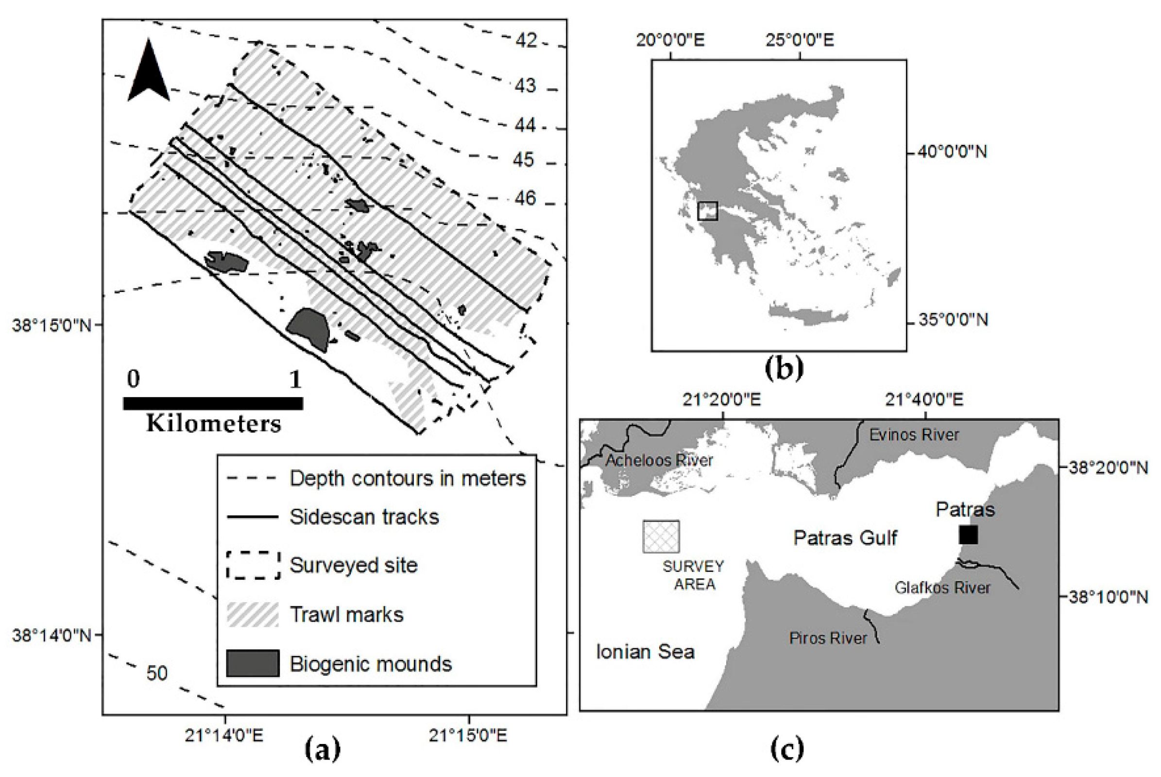
2.1. Study Area

The study area is located on the western end of the Gulf of Patras (western Greece, Mediterranean Sea), almost tangent to the geographic boundary line which separates the Gulf from Ionian Sea (Figure 1). The Gulf is an interconnected shallow marine embayment between Gulf of Corinth and Ionian Sea [58] and its deepest part lies at the depth of 135 m [59]. Pirros and Glafkos streams are the secondary sediment suppliers of Patraikos Gulf, complementary to the most important sediment provider, the Evinos River [58]. Fine sand and silt prevail close to river mouths which exhibit an ongoing fining trend as they move along into deeper water [58]. Sedimentation rate ranges levelly from 0.3 to 0.5 mm/year over the whole gulf [58]. The seabed of the study area is made up of Holocene clay and silt with high water content, indicating low energy sedimentation regime. Water circulation is mainly caused by wind-driven currents, at least in the winter months and tidal circulation in the Gulf of Patras is characterized by counter-clockwise direction [58]. Otter trawling is the most common method of fishing, targeting in soft sediments communities. The study area is estimated to be a bottom trawler fishing ground-hot spot for 7–8 of the 15 most important commercial species in Greece [60]. Due to the physical and mechanical properties of the sediments, TMs are expected to remain as visible linear seafloor disturbance for long period taking also in consideration that the fishing season lasts for 6 months (November-April) every year. Moreover, the study area is considered as an area of important archaeological significance as the crucial Lepanto Naval Battle took place in the area, in 1571, between Holly League Navy and the Ottoman Navy. Although Throckmorton et al. [61] suggested, through acoustic imaging, that there are scattered targets in the area that are likely ship remains from the battle, recent work by Patsourakis et al. [24] showed that those targets are nothing but biogenic mounds.

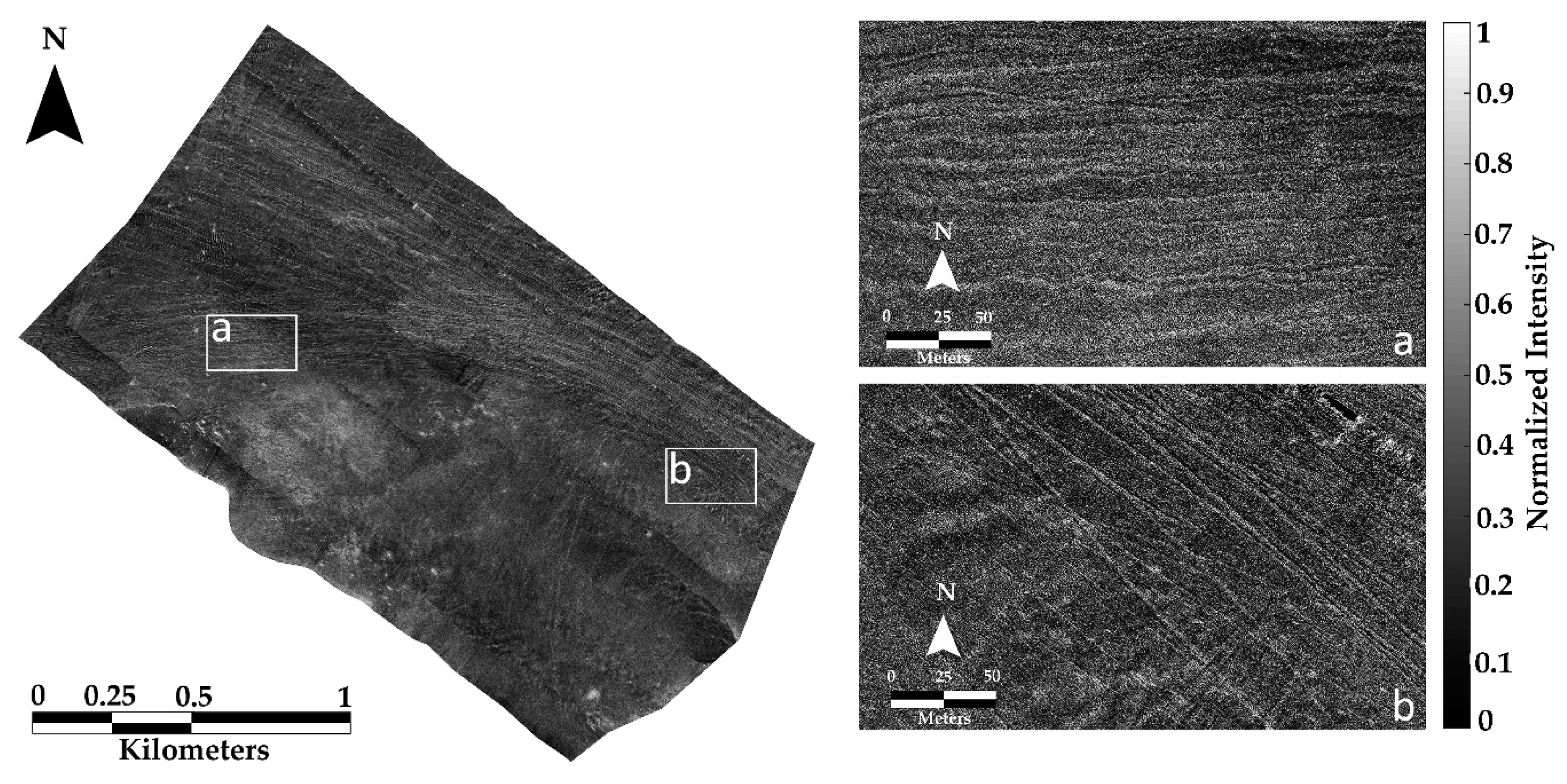
2.2. Data Acquisition and Processing

The survey took place in September 2006, after a closed trawl-fishing season of 6 months. The survey was conducted in a parallel-pass survey design to produce an SSS mosaic with 100% coverage of the seafloor. Six tracks were required (with a total length of 13.962 km) to cover an area of 2.98 km². The bathymetry in the research area is gradually increasing from −42 m to the northeast to −53 m in the southwest. Acoustic backscatter data of the seafloor were acquired with an EG&G 272TD sidescan towfish, connected to a top-side processor unit (EdgeTech 4200-P) with the data acquisition software Discover (EdgeTech). The sonar towfish was towed at an average height of 45 m above the seafloor and was operated at a sound pulse frequency of 100 kHz. A Hemisphere VS101 GPS system was used for the positioning of the research vessel. The position of the SSS towfish was calculated through the hypotenuse formula taking into account the cable-out and the towfish depth. Due to technical problems, only the right channel of the towfish was in operation and thus the survey-lines were adapted accordingly to achieve the desired overlap (20%) between the corresponding swaths. The swath range was set to 200 m and the ship speed ranged between three and four knots.

Data processing and mosaicking was performed using the “Isis” and “Tritonmap” softwares (Triton Imaging Inc.). Basic radiometric and geometric corrections were applied to the SSS records, including slant-range and Time Varying Gain (TVG) corrections respectively. The produced mosaic (Figure 2) has a pixel size of 0.2 m and dimensions of 13.380 × 12.056 pixels.

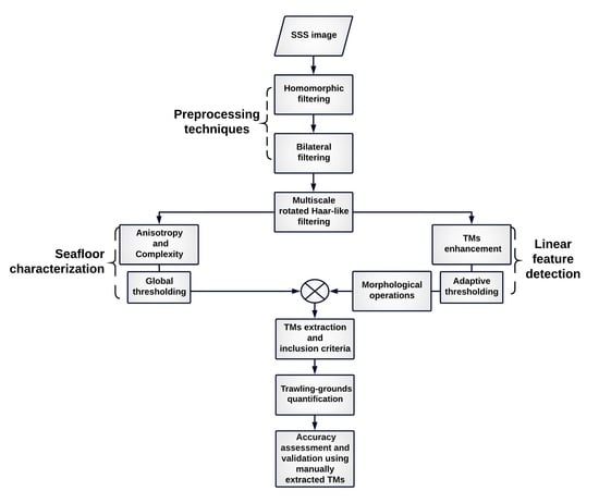
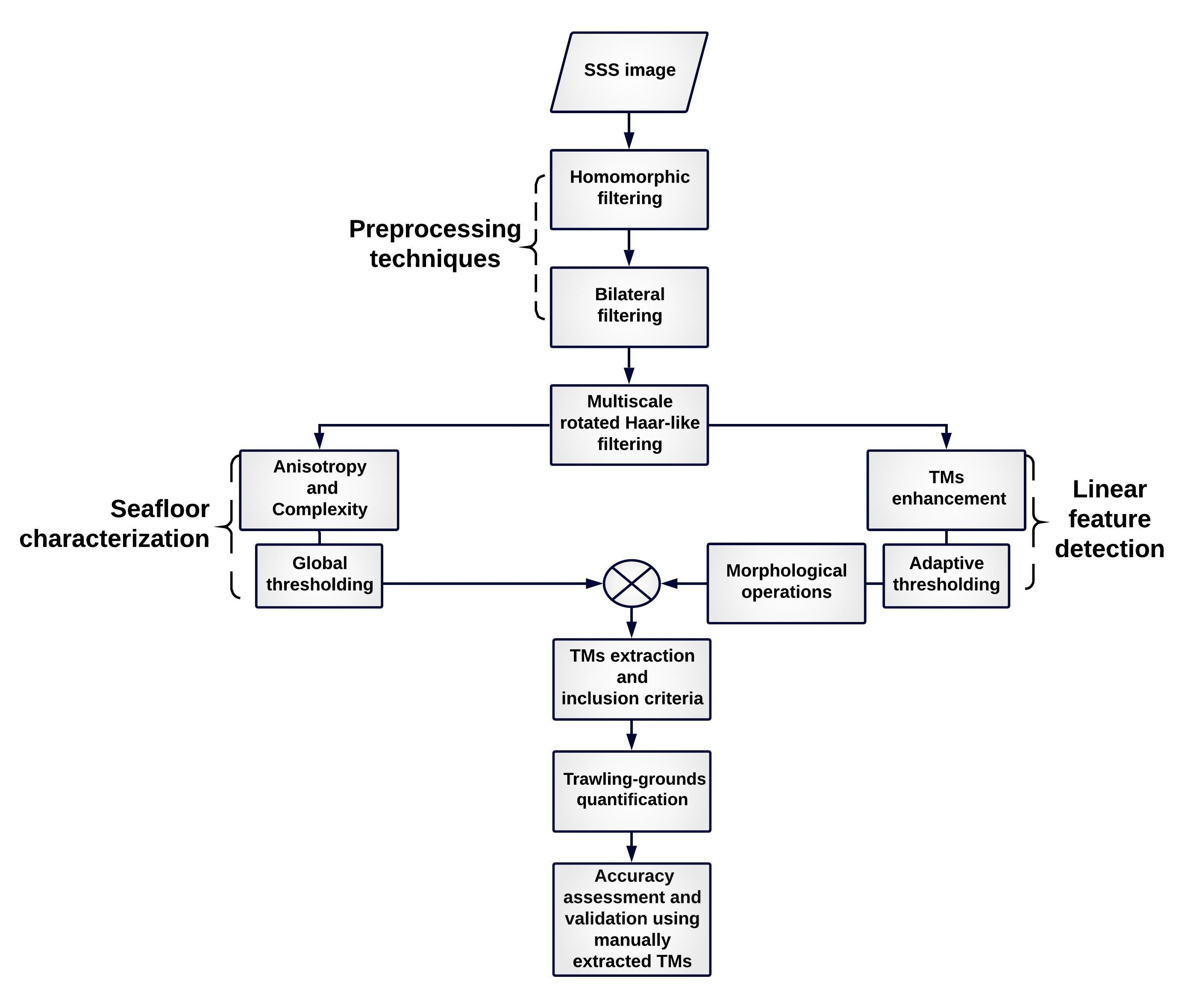
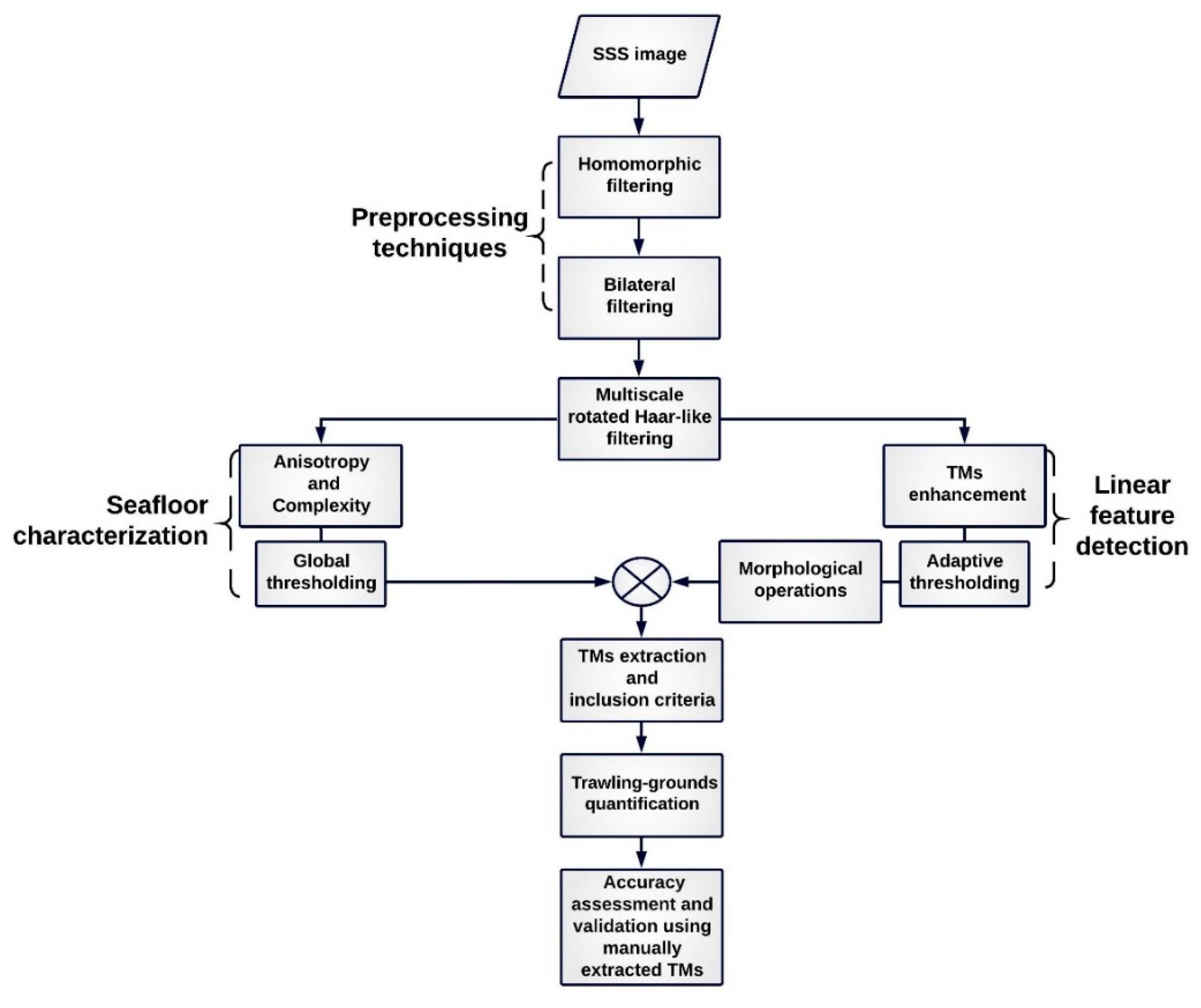
3. Methodology Overview

A multi-stage algorithm was implemented for automated TMs extraction and fishing ground quantification. This method applies spatial domain filtering and morphological operations to achieve an environmentally adaptive TMs detection and quantification, taking into account both TMs morphology and background seafloor type aspects. The procedure begins with subdividing the image into partially overlapping (sliding) blocks for computational efficiency. Our initial concern was to compensate image noise and amplitude inconsistencies, reform the visual information content of the backscatter images, and then proceed to a more in-depth analysis. Bottom-fishing grounds produce a monadic anisotropic seafloor type described as an otherwise flat seabed form with intense presence of long slightly curved lines [43]. In the main stage of the algorithm, we use Haar-like features that are capable of measuring the contrast between two adjacent areas of the seafloor. We followed work of Fakiris et al. [62] which used spatial domain filtering with Haar-like features for detecting anisotropic (oriented textures e.g., sand ripples) and complex (e.g., scattered rock - clutter) seafloor areas. Spatial domain filters, such as those based on Haar-like features, provide continuous metrics, which have explicit meanings, correlated to certain—consistent sea bottom characteristics, such as its level of Anisotropy and Complexity under certain scales. Those methods provide filter response maps that can be segmented using simple thresholds into accurate delineations of very specific bottom types. Fakiris et al. [62] used window averaged responses of the Haar-like filter to assess Anisotropy and Complexity definitions. In this study, effort has been put to designing a new filter with the use of the raw Haar-like filter’s responses in order to scale down the analysis and achieve feature–level segmentation of sub-meter analysis. The responses of the new filter lead to robust TMs detection by producing a map which highlight the locations of the linear seafloor features. The produced response-map is appropriately binarized and morphologically processed, and the TMs are extracted through an inclusion-exclusion procedure accordingly to their geometric, morphological and textural characteristics. Finally, fishing grounds are quantified in terms of the density, total length and direction of the TMs that they include. The evaluation of the proposed method’s performance was carried out by comparing the automatically extracted TMs with manual. All involved methods were implemented in MATLAB programming tool. The overall methodology workflow is presented in Figure 3.

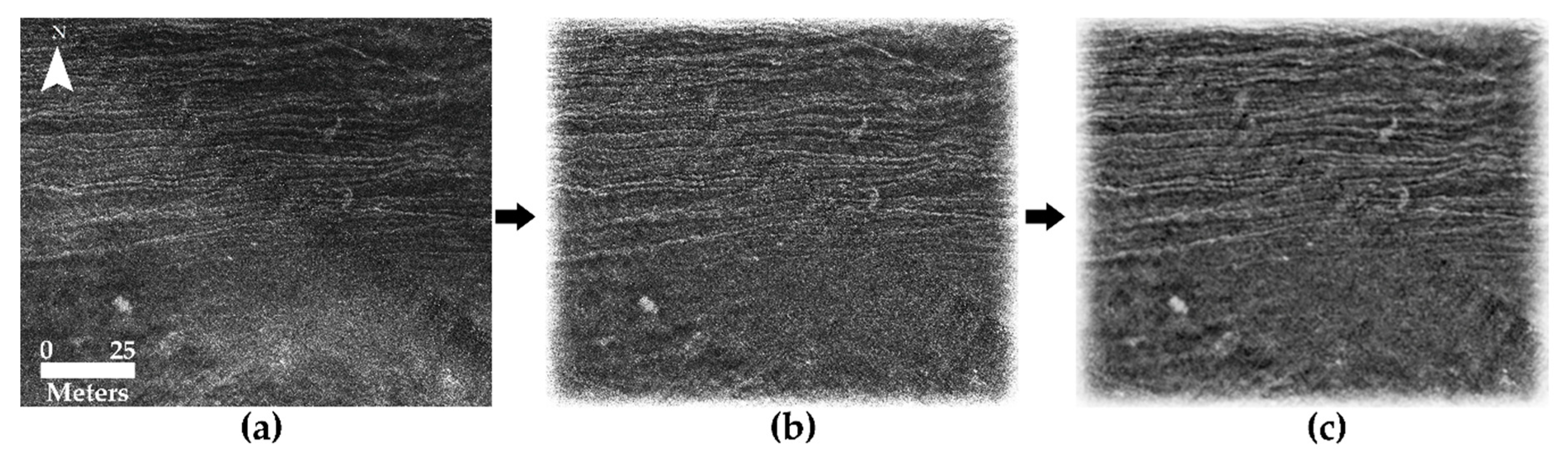
3.1. Preprocessing Techniques

3.1.1. Intensity Normalization

Homomorphic filtering, a frequency filtering complementary to an illumination-reflectance model, is applied to control the misbalance of intensity and strength the further processing. Image parts are the reflectance component and the illumination intensity component, described by a multiplicative relationship:

$$f\left(x,y\right)=i\left(x,y\right)r\left(x,y\right)$$

(1)

where $f\left(x,y\right)$ represents an image, $i\left(x,y\right)$ is the illumination factor and $r\left(x,y\right)$ is the reflectance factor [63]. Illumination varies without jerking though the field of view generating low frequencies, unlike the reflectance which abruptly changes and is associated with high frequency components [64]. The homomorphic filtering technique suppresses low-frequency components and is constituted of the following five steps [65] :(1) taking the logarithm of equation (1) allows the transformation of the multiplication operation to addition operation, (2) the Fourier transform of the log-image is applied to provide the image into frequency domain,(3) is achieved the elimination of the low frequencies by the use of a high-pass Gaussian filter, (4) returning to the spatial domain variants of the frequency domain filters by the evaluation of the inverse Fourier-transform, and (5) the exponential function is computed to obtain the filtered image.

3.1.2. Edge Preserving Smoothing

At the second step, we utilize bilateral filtering with Gaussian kernels which is implemented at the output image of the Homomorphic filter and offers edge-preserving smoothing (Figure 4). Bilateral filtering was introduced by Tomasi and Manduchi [66] and is a compromise between complexity and drastic denoising in cluttered imagery. It is a non-linear filter which is synthesized by domain and range filtering. Bilateral filtering run through the image pixel by pixel, replacing every pixel with a weighted average of the pixels that are close spatially and photometrically with it [67]. Combined filtering for the point x and a nearby point ξ is given by [68]:

$$B_x=\frac{1}{K\left(x\right)}{\displaystyle \sum }_{\xi \in \Omega }f(\xi ,x)g\left(I_{\xi },I_x\right)I_{\xi }$$

(2)

• $\Omega$ is the whole image,
• $I$ symbolizes the intensity,
• $f$ is the spatial gaussian kernel $f\left(\xi ,x\right)=e^{-\frac{1}{2}{\left(\frac{d\left(\xi ,\chi \right)}{{\sigma }_d}\right)}^2},$
• where $d\left(\xi ,x\right)=d\left(\xi -x\right)=\left|\left|\xi -x\right|\right|$ is the Euclidean distance between ξ and x,
• $g$ is an edge stopping function in intensity domain $g\left(\xi ,x\right)=e^{-\frac{1}{2}{\left(\frac{\delta \left(\xi ,\chi \right)}{{\sigma }_{\delta }}\right)}^2}$ where
• $\delta \left(I_{\xi },I_x\right)=\delta \left(I_{\xi }-I_x\right)=\left|\left|I_{\xi }-I_x\right|\right|$ is the distance between the two intensity values $I_{\xi }$ and $I_x$, and $K\left(x\right)$ is a normalization constant:
• $K\left(x\right)={\displaystyle {\displaystyle \sum }_{\xi \in \Omega }}f(\xi ,x)g\left(I_{\xi },I_x\right).$

3.2. Seafloor Characterization and Linear Seabed Feature Detection

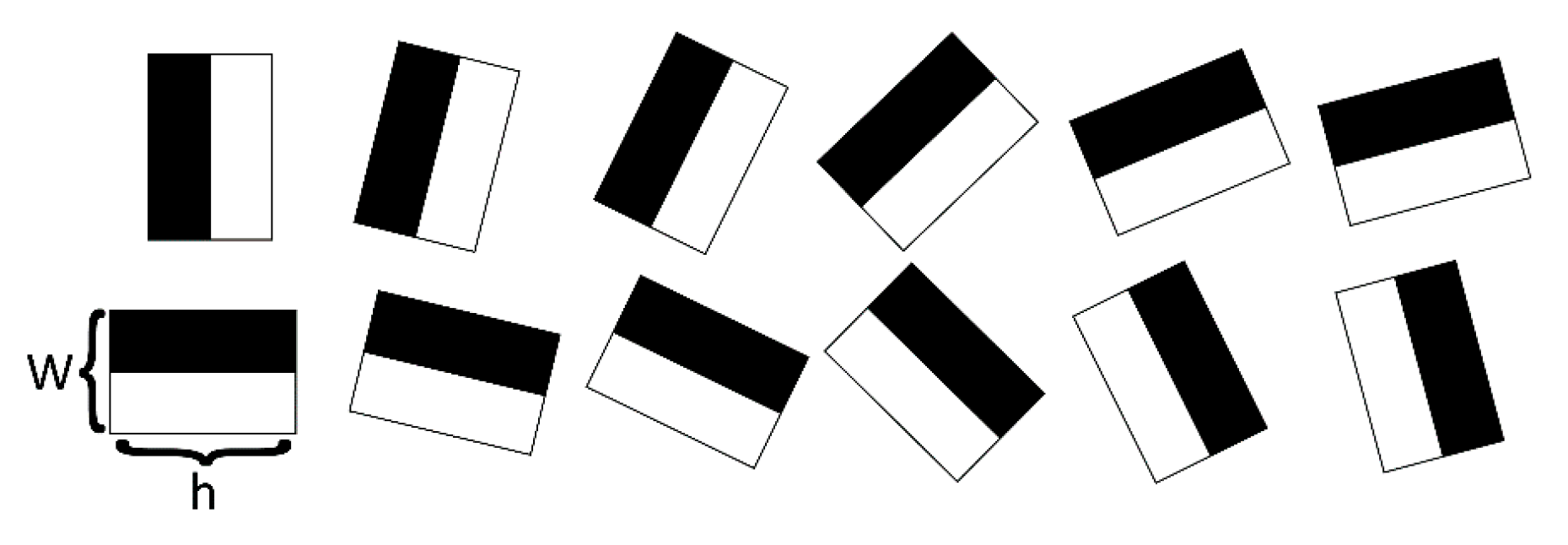
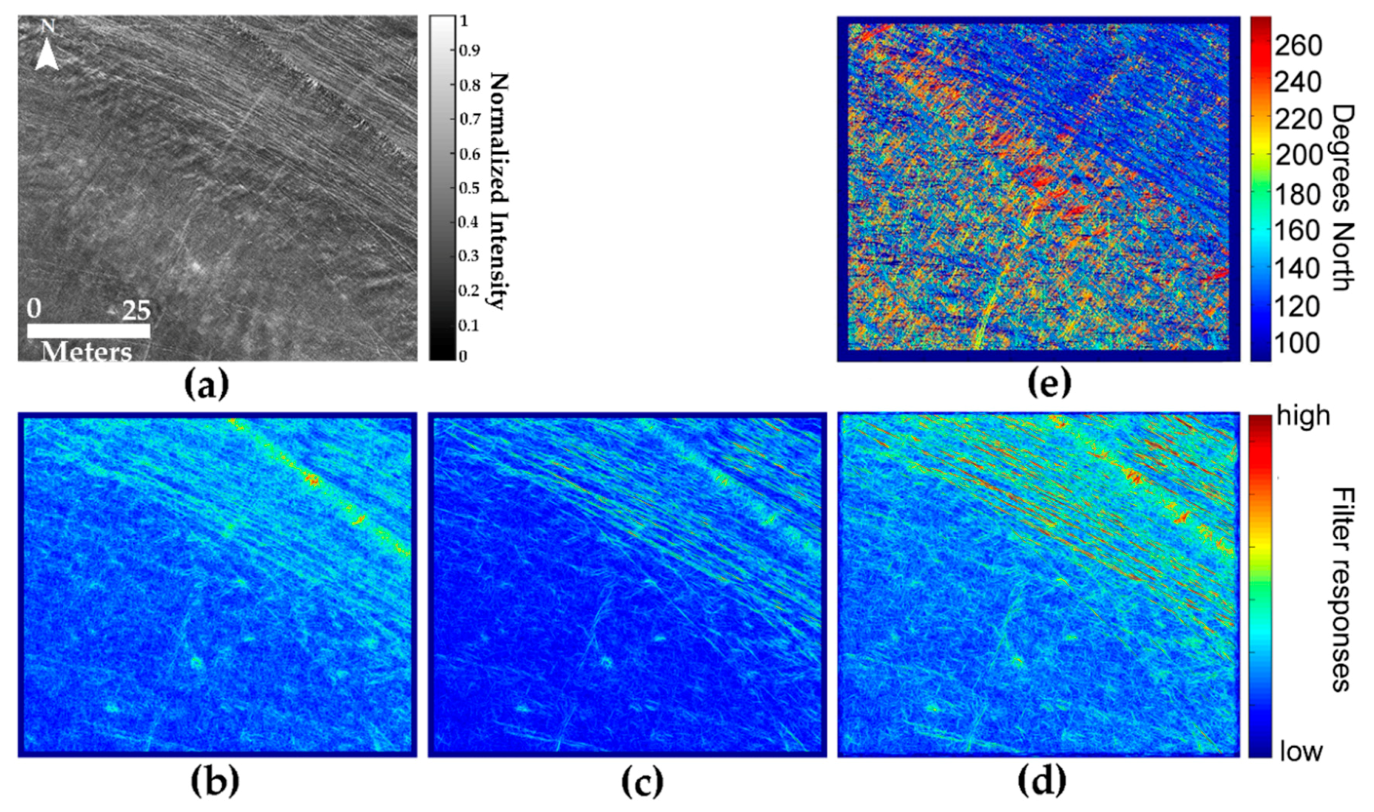
3.2.1. Multi-Scale Rotated Haar-Like Features

Haar-like features consist of white and black rectangles whose union is a rectangle. A Haar-like structure is represented as 0s and 1s in a geometrical order and the filter’s response is calculated as the subtraction of the summation of white subregions from the summation of the complementary subregion. Haar-like features have the advantage that they can be calculated directly from an integral image, speeding significantly up data processing. Normal Haar-like features were developed by Viola and Jones [69], their use had spread rapidly but those are not rotation invariant. Various rotated Haar-like features methods have been presented, including that of Fakiris et al. [62] that covers twelve rotations (Figure 5) and is sufficient for depicting features of almost any orientation. The rotated integral image, for a given integer rotation, is calculated by summing the pixels in the relevant aligned quadrant above the given pixel.

Intensity contrasts refer to neighbor areas that have certain spatial relationship (e.g., certain distance between them). As far as the spatial relationship is concerned, the scale under which the analysis is performed must be specified a-priori. In our case, two-rectangle rotated in twelve angles Haar-like features are able to depict the highlight-shadow scheme of TMs and delineate the various seafloor textures. For a more information-rich result, we implement a multi-scale, rotated Haar-like feature. We utilize a sequence of rotated two-rectangle Haar-like features with common aspect ratio but whose widths respectively correspond on terms of an arithmetic progression. The following function allows to determine the width w and the height h of the sequential Haar-like features:

$$s\left(i\right)=\left(w,h\right)=\left(z+\left(i-1\right)d, \alpha z+\left(i-1\right)\alpha d\right)$$

(3)

where i is the ordinal number of each rectangle in the sequential order of Haar-like features, α is the ratio of height to width, z is the width of the first rectangle and d is the common difference between the widths of the rectangles. For this case, the height of the smaller feature is 12 m and its width 0.6 m. The height of the second feature is 16 m and its width 0.8 m and the last one has dimensions 20 m and 1 m.

Next subsections’ filters are performed for each designed scale (s) of the set of Haar-like features with width (w) and height (h), rotated at direction k, that measure the contrast (c) between two adjacent oblong areas of the seafloor. High values of contrast show that the texture exhibits high differences between local intensities while low ones indicate uniform texture with little or no tonal changes. Local contrast $C_0$ can be expressed as the mean of differences (in grey levels) or as a percentage if normalized by the maximum value that intensities can take. Local contrast normalization for a fixed rotation k and scale s, is defined as is given by [70]:

$$C_{s,k}\left(x,y\right)=\frac{\left|C_{0_{s,k}}\left(x,y\right)\right|}{R}$$

(4)

where R is the intensity range (e.g., 256 for an 8-bit grayscale image) and $C_{s,k}\left(x,y\right)\in \left[0,1\right]$. Statistical measures are also constructive for our method such as the maximum, the average (μ_s,n) and the standard deviation (σ_s,n) of local contrast along a set of n directions, that are described by Equations (5)–(7) [70] and an example of their implementation is presented in Figure 6:

$${\mu }_{s,n}\left(x,y\right)=\frac{1}{n}{\displaystyle \sum }_{k=k\left(1\right)}^{k\left(n\right)}{C}_{s,k}\left(x,y\right)$$

(5)

$${\sigma }_{s,n}\left(x,y\right)=\sqrt{\frac{1}{n}\left[{\displaystyle \sum }_{k=k\left(1\right)}^{k\left(n\right)}{(C_{s,k}\left(x,y\right)-{\mu }_{\mathrm{s},n}\left(x,y\right))}^2\right]}$$

(6)

$$max{C}_k\ge C_k,\forall k\in \left[1,n\right]$$

(7)

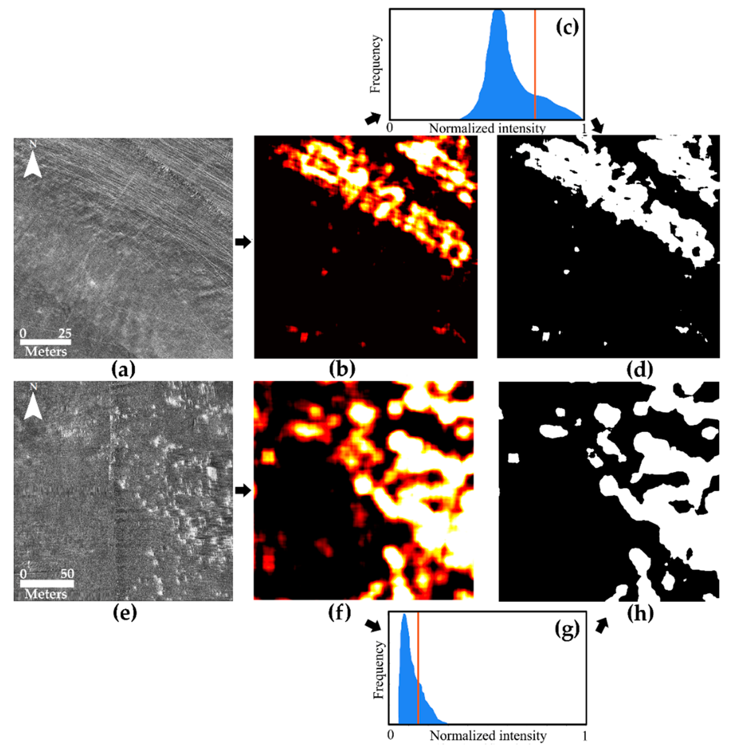
3.2.2. Seafloor Characterization

Texture can be described according to its two main characteristics: its contrast and orderliness, forming two groups of qualitative terms Image texture, defined as a function of the spatial variation in pixel intensities, is a topic investigated by many researchers in the last few decades [48,52,71]. A common application of image texture is the recognition of image regions using texture properties. The textural properties can characterize a seafloor region as rough or smooth, varied or homogeneous, repetitive or random, and hence can help in distinguishing between different areas and features in the images. Haar-like features’ filtering can be used to quantify both contrast and orderliness, as a single feature can assess the local variation of intensities but also highlight certain pre-specified structural geometries.

A square moving average filter is implemented with edge dimensions equal to the height (h) of the Haar-like feature that calculates the local averages of μ (called M) and σ (called Σ) filter’s responses. Based upon the above local averages of filter responses, two seafloor characterization measures: anisotropy and complexity, have been estimated, that are described thoroughly in [62]. The anisotropy A_s,h,k is equal to the square of the averaged standard deviation (Σ) to the averaged mean (M) ratio of filter responses over a set of k directions [62]:

$$A_{s,h,k}\left(x,y\right)={(\frac{\Sigma }{{\rm M}})}^2$$

(8)

Anisotropy refers to the level of heterogeneity of filters’ responses given for each direction [72] and therefore high values of anisotropy indicates that at least one direction responses overrides the others. Opposingly, when there are no poles apart in filters’ responses regarding to their direction, anisotropy is low valued. The complexity is equal to the square average (μ) to the standard deviation (σ) ratio of the filter responses over the set of k directions [62]:

$$C_{s,h,k}\left(x,y\right)=\frac{{{\rm M}}^2}{\Sigma }$$

(9)

The complexity filter highlights the high-contrast areas where seafloor features are anarchical distributed with respect to their direction. The combination of anisotropy and complexity allows the separation of the area into three seabed types: complex, anisotropic and featureless. The anisotropy and complexity threshold values that discriminate the three types of texture were set manually by the human interpreter, pre-trained using a small part of the dataset.

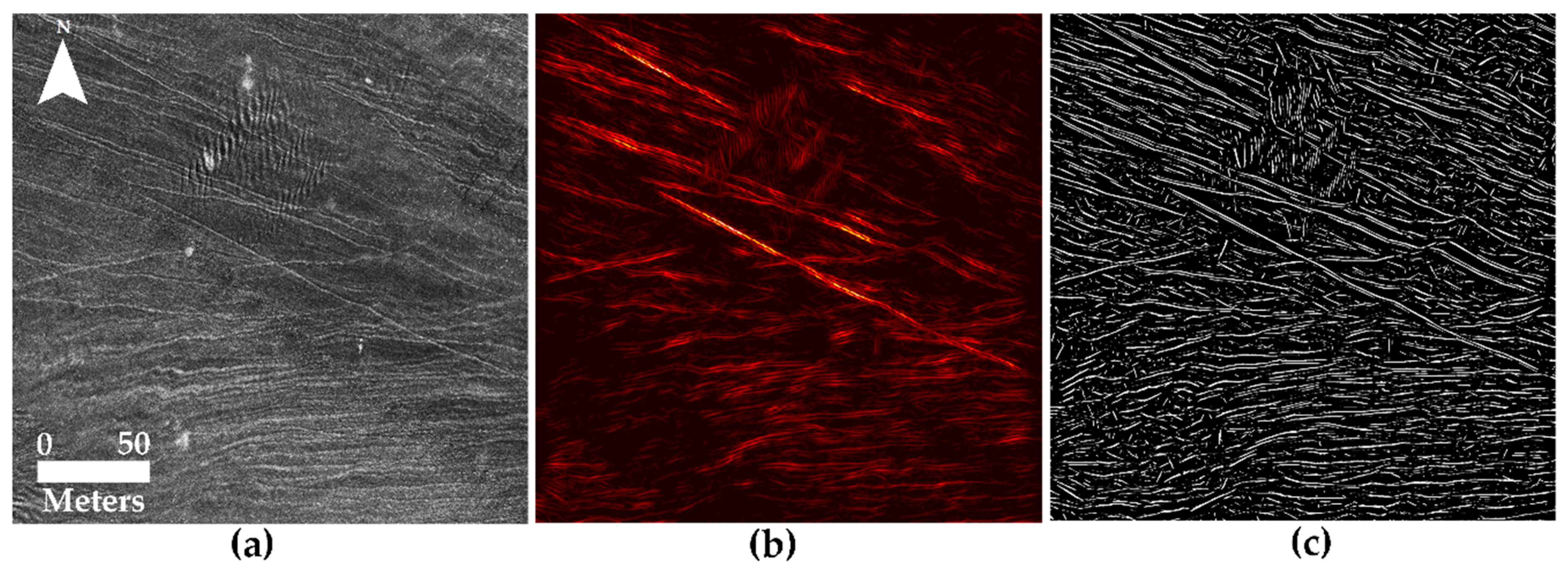
3.2.3. Linear Seafloor Feature Detection

The second utility of multi-scale rotated Haar-like features concerns linear seafloor features detection (segmentation). As the two-rectangle window slides in twelve directions, any linear edge is effectively depicted. A function over the filter responses aims at enhancing the figure of the TMs. Trawl-marks enhancement filtering (TME) works for each pixel of the image block and is defined as:

$$TME={\left(MRF\right)}^2$$

(10)

where MRF (maximum response filter) is the maximum contrast over all directions. Figure 7b shows a filtering result. For the binarization of the produced map with the potential TMs, the Gaussian adaptive thresholding method is used in which the threshold value is a weighted average of the pixel values in a manageable sized neighborhood (x,y) around pixel x. The variable threshold (T) is computed by the convolution of the image with the Gaussian function [73]:

$$T\left(x,y\right)={\displaystyle \sum }_{k=-a}^a{\displaystyle \sum }_{l=-b}^{b}G\left(s,t\right)f\left(x-k,y-l\right)$$

(11)

and G is the Gaussian function with standard deviation τ: $G\left(x,y\right)=\frac{1}{2\pi {\tau }^2}{e}^{-\frac{x^2+y^2}{2{\tau }^2}}.$

For each scale of the rotated Haar-like features a binary image is produced with the potential TMs. The binary images are combined with the logical operation “union” that synthesize a final binary image which contains each scale’s extracted TMs.

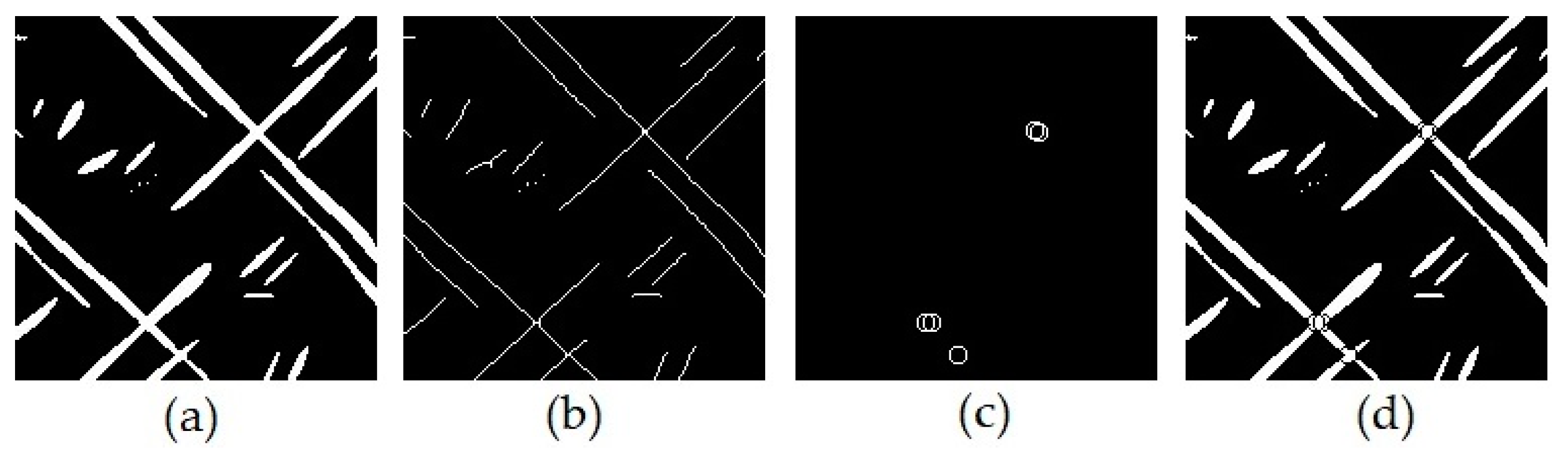
3.2.4. Splitting Lines at Intersections through Morphological Operations

All white connected pixels in the binary image are labelled as unique linear foreground objects and their properties are measured, such as their length and their orientation. The crossed lines are split and separated before the orientation of the identified objects is computed. The splitting of the lines is achieved through logical and morphological operations. Line skeletonization produces a thinned center line with respect to the length and the connectivity of the original linear object [64]. Skeleton shape facilitates the localization of the set of the intersection points. The points where the lines meet, are dilated and converted to circles in order to overlay the start points of the branches of any possible orientation. The set operation “difference” follows, and the circle-shaped structuring elements are subtracted by the primary binary image. In this way, the perimeters of the line junctions are thrown away from the original binary image and unlinked section lines are revealed. Figure 8 below presents each step of the lines spitting method.

3.3. TMs Extraction through Geometric and Textural Criteria, and Trawling Grounds Quantification

Via the feature space we seek to substantiate which line structures correspond to TMs. TΜ selection is designed based on an object’s geometric signature and the background environment features in the affected area. Following, this is a set of criteria that narrows the detected linear features down to those corresponding to TMs have been designed. The first geometric discrimination of the lines of interest is built upon their physical size. Lines with length more than 10 m are kept for further analysis. Additionally, we excluded line segments that have orientation perpendicular plus-minus 5 degrees from the survey line. As for the textural criteria, objects in the image whose Anisotropy background values lie under the manually chosen threshold are excluded from analysis. Moreover, areas that are characterized by high complexity are deleted from the regions of interest.

The example given here (Figure 9) is based on both geometric and textural criteria.

The final binary image is divided into 50 × 50 m blocks and their linear elements are analyzed statistically. The statistical analysis includes extraction of: (i) the density of the detected TMs (counts per area unit), (ii) the total length of the detected TMs per area unit and (iii) the mean per block orientation of the detected TMs. These parameters can be directly correlated to the fishing effort applied to a seafloor area.

4. Validation Data and Accuracy Assessment

The automatic TMs extraction results were evaluated using a dataset of manually extracted TMs. The results obtained by Patsourakis et al. [24] has preceded this, in which the same data were processed, and each individual TM was extracted manually, delineated and mapped on ArcGis software. The vector data of the manually digitized TMs were undergone spatial analysis to derive their mean density, length and direction per 50 × 50 m square area. These results are used as validation data and are compared to the results of the proposed method to assess its significance. Blocks were classified into four classes according to the TMs’ total length. The first category includes the blocks that do not contain any TMs, the second category includes the blocks with total ΤΜs length less than 200 m, the third category contains the blocks with total length between 200 and 400 m and the last category includes the blocks with total length greater than 400 m. A cross tabulation matrix is used to evaluate the one-to-one correspondence of the classes and to identify a possible relationship between two different classes. The Cohen’s kappa coefficient evaluates the agreement between the corresponding class limits who each classify the blocks into the four mutually exclusive categories and can range from 0 to +1.

Accuracy of automatic TMs detection method is evaluated by comparing the two data sets that are defined by thresholds of the total TMs length that are used as binary classifiers. If a block contains a number of total TMs length bigger than the threshold it is considered as ‘positive’ block else is considered as ‘negative’. Depending on whether respective blocks of manually and automatically derived TMs coincide in their ‘positive’ (positive/positive) or ‘negative’ (negative/negative) characterizations correspond to ‘true positive’ (TP) and ‘true negative’ (TN) sections which indicate an equivalence relation between the data sets. Otherwise, when the blocks are oppositely characterized (positive/negative or negative/positive) correspond to ‘false positive’ (FP) and ‘false negative’ (FN) sections that point out commission and omission errors, respectively. For each class, the number of the TP, TN, FP, FN determine the sensitivity (or recall), specificity, precision and accuracy measurements that are shown in Equations (12)–(15):

$$Sensitivity=\frac{TP}{TP+FN}$$

(12)

$$Specificity=\frac{TN}{TN+FP}$$

(13)

$$Precision=\frac{TP}{TP+FP}$$

(14)

$$Accuracy=\frac{TP+TN}{TP+TN+FP+FN}$$

(15)

Sensitivity, specificity, precision and accuracy measurements can range between 0 and 1, where 1 represents perfect correspondence between the length quantification values of the classified data sets, and 0 indicates failure.

5. Results

5.1. Data Interpretation and Seafloor Characterization through Anisotropy and Complexity Definitions

The interpretation of the 100 kHz side scan sonar mosaics revealed three distinct acoustic backscatter patterns in the survey area: (i) uniform low-reflectivity seafloor, (ii) localized strong backscatter facies in low reflectivity seafloor that well matches with micro-relief seafloor areas, and (iii) numerous, long, linear to curvilinear and parallel to subparallel features on the seafloor with high reflectivity (Figure 2). The first acoustic backscatter pattern represents fine grained sediments (clay, silt and fine sand). The second one represents high reflectivity mounds. Ground truthing survey showed that those mounds are biogenic mounds (Figure 2). These biogenic mounds are quite similar to the coralline algae reefs that have been reported in the Eastern Mediterranean Sea (Aegean Sea) by the authors of [13]. The linear features of the third acoustic pattern are interpreted as marks produced by bottom-fishing gear (TMs) (Figure 2).

Planar seafloor is characterized by the absence of directional features and is represented by low anisotropy values while a trawled seafloor area gives high values of anisotropy [62], as presented in Figure 10. Biogenic mounds, bedrocks and scattered boulders synthesize a seafloor area that corresponds to high complexity. The combination of anisotropy and complexity allows the separation of the area into three seabed types: complex, anisotropic and featureless. Setting a well-suited threshold, complex areas can be easily selected and fully represented as shown in Figure 10. Anisotropy thresholding creates two zones: above the threshold stand the anisotropic areas and below of it, the benign seabed. Planar seabed and anisotropic-complex zones are mutually exclusive. As well, complex areas are not strongly correlated with regions that contain TMs.

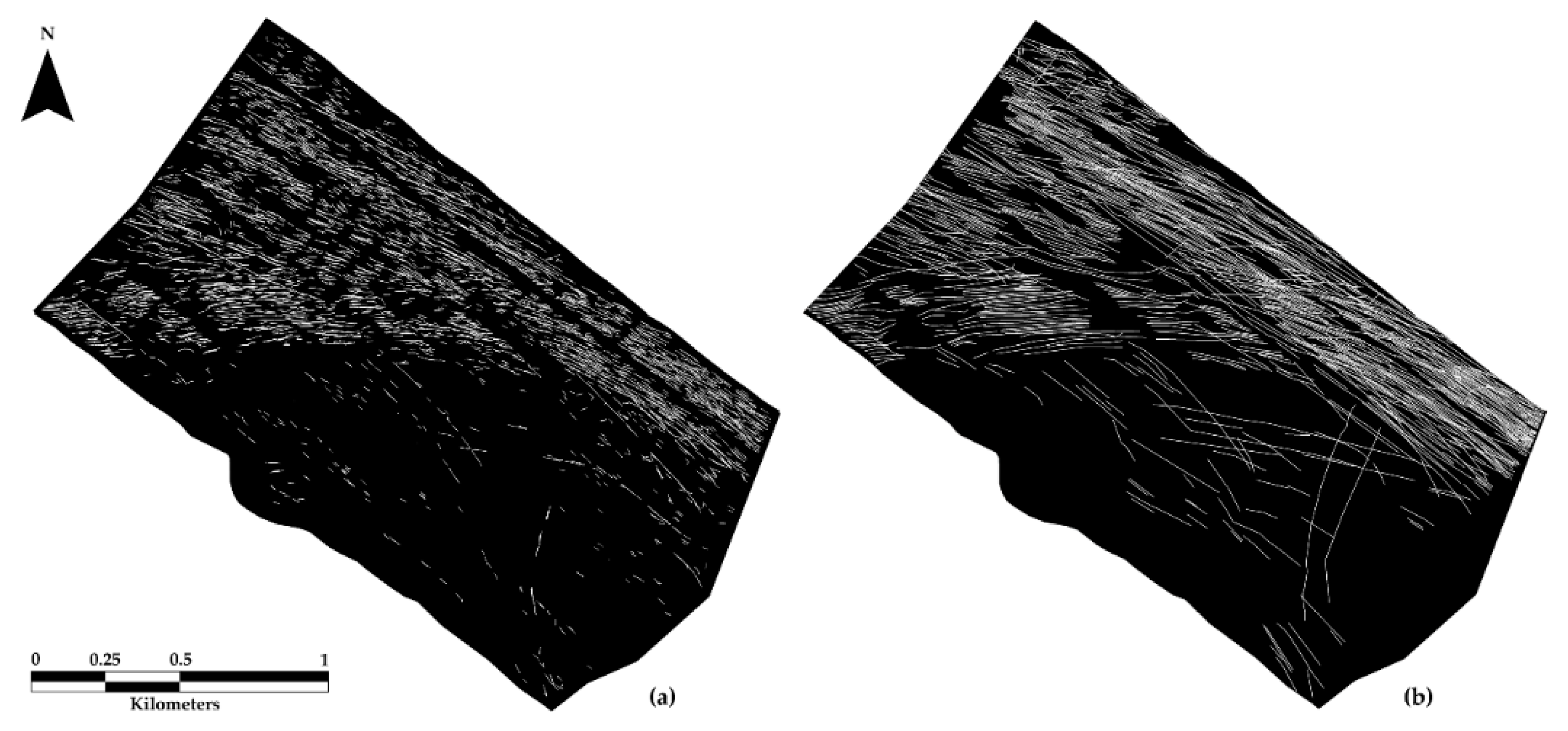
5.2. Trawl-Marks Extraction and Quantification

The spatial scale analysis of the detected TMs has a significant impact on interpreting effects of bottom-fishing. The statistical results of the spatial quantification of TMs length are reported in

Table 1. Results of statistics on the quantification values of TMs length. The analysis calculates statistics for the blocks that contain TMs.

Descriptive Statistics	TMs Length Automatic Method	TMs Length Manual Method
Min (m/km2)	392	896
Max (m/km2)	86,176	90,493
Mean (m/km2)	25,369	26,226
Total TMs in whole area (m/2.98km2)	53,212	51,960

. The results were calculated per 25 × 10⁻⁴ km² and then converted per km².

The proposed algorithm was applied in sliding blocks of the backscatter mosaic to achieve lower computational-cost. The automatically detected TMs are shown in Figure 11a. The main aim of this study was to derive density maps that visualize the fishing stress and the preferred axles of towing. In Figure 12 vectors, TM density maps, and rose-plots are presented both for the automatic and manual TMs digitization cases, giving the means for visual comparison and qualitative accuracy assessment.

5.3. Accuracy Assessment

The accuracy assessment results of the proposed approach are reported in

Table 2. The accuracy assessment results. Cases correspond to total TM length per analyzed block.

Categories	Cases	TP	TN	FP	FN	Sensitivity	Specificity	Precision	Accuracy
Classes	0	318	755	19	84	0.79	0.98	0.94	0.91
	<200 m	655	361	103	57	0.92	0.78	0.86	0.86
	200–400 m	108	796	95	117	0.38	0.89	0.53	0.77
	>400 m	104	886	111	75	0.58	0.89	0.48	0.84
Existence—absence		755	318	84	19	0.98	0.79	0.9	0.91

. Accuracy exhibited high values, ranging from 77% to 91%, with the highest values being met in the “0” and “>400” classes as well as in the “TM existence—absence” case. Precision and Sensitivity were lower at the third and fourth cases of high total TM lengths, indicating that those length ranges exhibit average agreement to the manually digitized equivalents. The accuracy assessment results of the first and last classes (“0” and “>400 m”) as well as the very high accuracy of the “TM existent-absence” binary case, shows that the proposed method can provide accurate quantitative results for highly trawled areas, but it can also separate impacted from non-impacted ones. What is more, the proposed method manages to determine TMs directions with very high precision, as shown in Figure 12c,d.

The cross-tabulation matrix of the four classes (regarding certain ranges of total per unit area TM length) is shown in Figure 13a. The diagonal in the cross tabulation has the greatest concentration of scores indicating consistency and stable correlation between the corresponding classes of the two datasets. The class ‘0’ has a 94% agreement, conveying that FP rates are almost entirely suppressed at the areas where TMs do not exist. In classes with higher TMs densities there is a good agreement between the manual and automatic TM densities. The Cohen’s kappa coefficient is equal to 0.65, indicating a substantial agreement of all class ranges that are used to classify the blocks of the manually and automatically derived TMs. The automatically and the manually extracted TMs have the same spatial distribution when blocks are given 0–1 values (TM absence—presence), where the accuracy value is greater than 0.9 (Figure 12b). This implies that fishing grounds, as a bottom-type, can very accurately be detected through the proposed method.

High accuracy values are in the diagonal of the accuracy vs threshold diagram (Figure 13b), indicating highly accurate results as the total-length threshold increases (excluding more and more low TM density areas from the analysis). This graph was made to be interpreted as the sensitivity of the method to noise, i.e., to areas with few scattered linear element detections that could potentially be false detection (noise). However, the fact that very low thresholds (no or limited exclusions) have comparatively better accuracies suggests that even areas with very few TMs are very well segmented and do not need to be considered even partially false. The agreement between the manual and the automatic TMs assessment is strong (>0.9) up to the threshold of 240 m, after which the accuracy has a slight decrease, and it is improved after 400 m total TM length per unit area. This threshold range between 240 and 400 m indicates that there is a factor limiting the accuracy of the method in blocks that are within this range, which is most likely correlated with the northwest area where the worst agreement between manual and automatic TMs assessment is met, due to increased deviation between the TMs’ and survey lines’ orientations, as discussed in Section 6.

6. Discussion

The proposed algorithm enables the automatic detection of TMs that was previously unattainable due to the limitations of the data conditions and the environmental variable characteristics. The automatic TMs detection algorithm was performed in SSS images with high presence of noise, disfigurements and artifacts. The results reveal that the design of the algorithm overcomes the aforementioned limitations, achieving high accuracy in TMs detection and decreasing the false alarm rates. This image processing method was performed to the whole sonar mosaic providing quantitative estimation of trawling impacts on the seafloor. Returning to the aim of this study posed at the beginning of this paper, it is now possible to state that fishing activity had highly localized impact on the seafloor of Gulf of Patras (Table 1), a biologically significant marine area with historical and cultural relevance. The quantified TMs length values were used as a new indicator of pressure of bottom trawling.

The preprocessing stage was a necessary step that successfully normalizes the non-uniform intensity, suppresses the noise and at the same time gives at TMs a more discrete appearance in SSS image data. In reviewing the literature, many prior studies in this field [74,75] have noted the importance of using an uniform backscatter intensity mosaic. Radiometric and geometric corrections is an issue of high importance in acoustic imaging, but in SSS data, where there is no auxiliary information about the exact geometry of the ensonification, their elaboration is difficult [73,76,77,78]. The proposed approach embeds a common technique in satellite and medical image processing for correcting non-uniform intensity, the Homomorphic filtering, which reverses the situation of hidden environment in images. Homomorphic filtering helps in TMs separation when the background backscatter intensities change in space, depending on the sediments properties, making TMs in low backscatter intensity soft sediment hardly separated. Considerable emphasis was also placed on the most conventional problem of sonar imagery, the injected noise. The acoustic backscatter images are getting acquired and transmitted under the presence of ambient noise [79]. Acoustic artifacts such as stripe noise by roll towfish motion or other electrical noise deteriorate the quality of the sonar image [80]. According to Wilken et al. [81] in most cases SSS mosaics are affected by visible stripe noise. Although stripe noise and the TMs differ in thickness, geometry and intensity, if we do not use an effective noise reduction filter, we jeopardize to set stripe noise as candidate line segments which may or may not be portions of TMs. Furthermore, the stripe noise engenders impoverishing and fragmentation of the illustrated TMs when they intersect. It is apparent from Figure 4 that bilateral filtering boosts TMs performance in the SSS data while noise is reduced.

The implemented algorithms exhibit low computational costs, utilizing calculations on integral-image, making it suitable for quasi real-time operations. Digital filters based on multiscale, rotated Haar-like features, proved to be capable of detecting TMs of great variability in curvature, orientations, intensities and contrasts. The smaller rotated Haar-like features can depict more precisely the step edges of a narrow line and fit better in curves of considerable torsion. The longer Haar-like features are able to highlight ramp edges and surpass small gaps of long linear edges. The binarization of the highlighted linear features and the splitting of the crossed lines were two of the key problems in this method. The lines splitting method was achieved in an accurate way by removing the nodes of the skeleton which satisfy high geometrical fidelity to the lines’ representation. The splitting of the lines allows the proper lines orientation measurement that is precious information for a set of operations in this method, such as the TMs quantification in terms of orientation.

Thresholding is one of the most important approaches in image segmentation. The most widely used thresholding method is to choose a single threshold value as assignment criteria [82]. Sometimes, the fixed thresholding method breaks down in complex images [83] as the weak edges, features and information are getting ignored [84]. To maximize the generalizability of the designed algorithm, we tried to make use as much as possible of adaptive thresholds [85], that require no human decision making to be involved in the process. However, our method still concerns a range of parameters that need to be defined manually. Some of them were set to their most bibliographically common ones (intensity normalization), offering adequate results. Others were determined using the well-defined geometries of the target seafloor feature (TMs), such as the Haar-like features, whose dimensions were adapted to common TM geometries met in sonar images. Still, very few parameters needed to be set in a heuristic. The latter are the Anisotropy and Complexity thresholds used for environmental adaptation through seafloor characterization. These thresholds are particularly sensitive to the ensonification geometries (incidence angles, towing-height above the ground) and the equipment used (transmit frequency) that control the shadow extents and the texture contrast of the TMs. However, those are simple thresholds and so they need no time-consuming training phases but rather a couple of sample areas to tune them suitably.

The SSS mosaic encompasses a combination of anisotropic areas with the intense presence of TMs and areas of featureless homogeneous soft sediments. The SSS mosaic also depicts complex areas that represent scattered biogenic mounds. A growing body of literature pays particular attention to the extent and the acoustic pattern of coralligenous formations [13,71,86,87]. Despite the fact that the EU 1967/2006 Mediterranean fisheries management Regulation protects the biogenic habitats, they are commonly impacted by fishing activities [13,88]. The presence of biogenic mounds creates areas of complex surficial geology which are accurately delineated by the Complexity filter. One unanticipated finding of this study was that there is no linkage of the trawling activity with the biogenic mounds according to the textural analysis and the data interpretation of the mosaic. This is most probably explained by the fishermen’s knowledge of this rigorous morphology of the seafloor and the consequent avoidance of surpassing them in order to protect their gears [24]. This is also reaffirmed by the turn of the trawl tracks on the northern boundary of the research area [24] (Figure 11a,b). TMs presence on seafloor implies tonal differences of adjacent image regions creating an anisotropic textured area [62] and seem to be uncorrelated with regions of featureless textural seafloor which is characterized by homogeneity. By implication, areas that are characterized by low Anisotropy constitutes non-TM regions. The implementation of Anisotropy filter facilitates the separation of the two different textures which consequently eliminate the number of false alarms at the zones where TMs are absent, as reaffirmed by the high precision score of the class ‘0’. TMs are described as long straight or slightly curved lines, sometimes parallel and equidistant. Boundaries of biogenic mounds produce sharp edges in sonar imaging that could be confused with TMs and therefore are excluded. Collectively, the information about the texture of the seafloor has a valuable impact on eliminating false alarms while no classifiers are needed for the seafloor characterization.

Seafloor linear structures are accurately visualized when the towfish fly parallel to their orientation, but may be not clearly depicted or hidden when the towfish track is perpendicular to their orientation [89,90]. In addition, a major part of the SSS image noise is in the across-track direction, caused by towfish movements (roll, pitch and yaw), electric and mechanical interferences. These factors contribute to the exclusion of the detected line segments that have orientation perpendicular ± 5 degrees from the survey line. Contrary to expectations, total 10⁰ degrees orientation exclusion is an appropriate way to achieve the right balance between a high level of noise-free mosaic and high accuracy in the TMs density estimation. Moreover, as TMs are appeared as long linear troughs [29] in SSS data, short lines are not selected as TMs. Short line segments may be a result of the interaction between high sensitivity of the adaptive thresholding and complex marine noise, inferior image resolution or inherently changes of the seafloor backscatter strength.

The data used in the present work was not acquired for the assessment of trawling activity, which would require higher acoustic incidence angles (proximity of the SSS towfish to the ground) but rather for a general-purpose, low-cost and time-limited seafloor research. The swath range was kept high (200 m) and as a consequence the acoustic signature of TMs has low contrast and under-developed acoustic shadows, hindering the quality of the produced mosaic. The direction of the survey lines was set constant, without any multi-angle view compensation. This way, TMs that run parallel to the survey tracks had a more vivid and clear depiction than the ones which stand at an increased angle [29,90], affecting the detection accuracy. Consequently, the design of this survey lacked some sidescan tracks, especially perpendicular to the tracks made, which would offer focused and safer TMs depiction by viewing them from different angles. Further elaboration on the reasons that hinder method significance in the present case study, revealed that the direction of the TMs in comparison to the direction of the survey lines plays an important role in TM detection accuracies. This is intuitively clear given that TMs and other proud linear features (such as sand-ripples) are more difficult to be detected when they get perpendicular to the swath direction, where their contrast and shadow length decreases. Figure 12a confirms the above hypothesis, showing an increased error per unit area as the deviation of the TM orientation from the survey-lines’ equivalent gets higher. The total TM length is slightly underestimated (<10%) when the orientation deviation is less than 35° but it is severely overestimated (up to 50%) for deviations higher than 35° (Figure 14). This finding is opposite to what one should expect, i.e., a decreased ability of the system to detect TMs as the direction deviation gets higher, leading to increasing their underestimation. This paradox can be interpreted in just one way: what is expected to bias computer aided detections is also biasing human-interpretation. It is true that there are cases within the present dataset where the human interpreter did not include intentionally, or even missed, some minute, controversial linear features that actually were TM parts, while the proposed method did.

Regardless of the above survey set-up and data suitability restrictions, application of the proposed fishing ground detection and quantification method exhibited high potentials. The overall accuracy of the method on separating trawl-impacted grounds from non-impacted ones was more than 90%, the general orientation of the TMs was very accurately determined, while a substantial agreement (Kappa = 0.65) between the manual and automatic total TM length per unit area was achieved. The results of this automatic TMs detection and quantification method show that trawling grounds can be detected irrespectively to the survey design. However, there are findings that indicate that the automatic assessment of fishing effort, quantified as increased TM lengths per unit area, were better determined using the proposed method rather than through manual interpretation. Nonetheless, future work should regard evaluation of the algorithm’s performance using SSS datasets from better adapted surveys to the general needs of target and object detection tasks.

7. Conclusions

In this paper a new method was presented that achieves automatic detection and spatial quantification of TMs under challenging conditions of acoustic imaging when general-purpose SSS data are used. The algorithm was demonstrated on SSS images of board-scale and structural complex habitats and successfully detected TMs of great variability with respect to orientation, intensity and contrast. This is the largest study so far documenting a delayed onset of automatic TMs quantification in terms of length and orientation, that is also characterized by high accuracy values. The integration of this image processing method in acoustic remote sensing, provides valuable information about the bottom fishing effort intensity and distribution. The approaches developed prove that there is definitely room for improvement in identifying fishing behavior of trawlers and in evaluating fishing impacts on the seafloor through SSS imaging. Spatiotemporal analyses of the exported data are expected to be useful for the prognosis of the ecosystem’s recovery trajectories in terms of trawling impacts.

A natural progression of this study is to implement some of its features in conjunction with machine learning principles through the use of extended sonar datasets of TMs. As in the case of other geological seafloor features (e.g., faults, land-slides, pock-marks etc.) though, open swath sonar datasets are still quite limited to meet the need for extensive training datasets that deep learning or other machine learning methods demand. A major factor for this is that sonars produce multi-aspect, multi-frequency views of the same seafloor target, depending on the acquisition parameters and the type of equipment used, and so a huge number of samples may be needed to adequately include all the possible versions of the same feature in the training dataset. In addition, backscatter intensity normalization is still a matter of negotiation among acousticians and so datasets between different users are not yet directly comparable. Although transfer learning is an intriguing option in recent deep learning applications, that could minimize the training-sets needed or even take advantage of extensive datasets in similar terrestrial applications (e.g., radarsat ), it still needs to be extensively validated against real sonar datasets before replacing traditional spatial domain filtering for seafloor feature recognition, as those used operationally in mine counter-measurement tasks [91].

References

1. Rosales, R.M.P. SEAT: Measuring socio-economic benefits of marine protected areas. Mar. Policy 2018, 92, 120–130. [Google Scholar] [CrossRef]
2. Sanchirico, J.N.; Cochran, K.A.; Emerson, P.M. Marine Protected Areas: Economic and Social Implications; No. 1318-2016-103151; Resources for the Future: Washington, DC, USA, 2002. [Google Scholar]
3. Bennett, N.J. Marine Social Science for the Peopled Seas. Coast. Manag. 2019, 47, 244–252. [Google Scholar] [CrossRef]
4. Russi, D.; Pantzar, M.; Kettunen, M.; Gitti, G.; Mutafoglu, K.; Kotulak, M.; ten Brink, P. Socio-Economic Benefits of the EU Marine Protected Areas; Institute for European Environmental Policy: London, UK, 2016. [Google Scholar]
5. Oberle, F.K.J.; Puig, P.; Martín, J. Fishing Activities. In Submarine Geomorphology; Micallef, A., Krastel, S., Savini, A., Eds.; Springer International Publishing: Cham, Switzerland, 2018; pp. 503–534. ISBN 978-3-319-57852-1. [Google Scholar]
6. Ramirez-Llodra, E.; Tyler, P.A.; Baker, M.C.; Bergstad, O.A.; Clark, M.R.; Escobar, E.; Levin, L.A.; Menot, L.; Rowden, A.A.; Smith, C.R.; et al. Man and the Last Great Wilderness: Human Impact on the Deep Sea. PLoS ONE 2011, 6, e22588. [Google Scholar] [CrossRef] [PubMed]
7. Woodall, L.; Stewart, C.; Rogers, A. Function of the High Seas and Anthropogenic Impacts Science Update 2012–2017; University of Oxford: Oxford, UK, 2017. [Google Scholar]
8. Merillet, L.; Mouchet, M.; Robert, M.; Salaün, M.; Schuck, L.; Vaz, S.; Kopp, D. Using underwater video to assess megabenthic community vulnerability to trawling in the Grande Vasière (Bay of Biscay). Environ. Conserv. 2017, 45, 163–172. [Google Scholar] [CrossRef]
9. Riemann, B.; Hoffmann, E. Ecological consequences of dredging and bottom trawling in the Limfjord, Denmark. Mar. Ecol. Ser. 1991, 69, 171–178. [Google Scholar] [CrossRef]
10. Robelly, M.; Beaman, R.J. Spatial analysis of seabed trawl marks, Frederick Patches, northern Great Barrier Reef. In Proceedings of the SEES Research Student Conference, Townsville, Australia, 1 November 2011. [Google Scholar]
11. Jones, J.B. Environmental impact of trawling on the seabed: A review. N. Z. J. Mar. Freshw. Res. 1992, 26, 59–67. [Google Scholar] [CrossRef] [Green Version]
12. Kiparissis, S.; Fakiris, E.; Papatheodorou, G.; Geraga, M.; Kornaros, M.; Kapareliotis, A.; Ferentinos, G. Illegal trawling and induced invasive algal spread as collaborative factors in a Posidonia oceanica meadow degradation. Biol. Invasions 2011, 13, 669–678. [Google Scholar] [CrossRef]
13. Georgiadis, M.; Papatheodorou, G.; Tzanatos, E.; Geraga, M.; Ramfos, A.; Koutsikopoulos, C.; Ferentinos, G. Coralligène formations in the eastern Mediterranean Sea: Morphology, distribution, mapping and relation to fisheries in the southern Aegean Sea (Greece) based on high-resolution acoustics. J. Exp. Mar. Biol. Ecol. 2009, 368, 44–58. [Google Scholar] [CrossRef]
14. Ingrassia, M.; Martorelli, E.; Bosman, A.; Chiocci, F.L. Isidella elongata (Cnidaria: Alcyonacea): First report in the Ventotene Basin (Pontine Islands, western Mediterranean Sea). Reg. Stud. Mar. Sci. 2019, 25, 100494. [Google Scholar] [CrossRef]
15. Brennan, M.L.; Davis, D.; Ballard, R.D.; Trembanis, A.C.; Vaughn, J.I.; Krumholz, J.S.; Delgado, J.P.; Roman, C.N.; Smart, C.; Bell, K.L.C.; et al. Quantification of bottom trawl fishing damage to ancient shipwreck sites. Mar. Geol. 2016, 371, 82–88. [Google Scholar] [CrossRef] [Green Version]
16. Krumholz, J.S.; Brennan, M.L. Fishing for common ground: Investigations of the impact of trawling on ancient shipwreck sites uncovers a potential for management synergy. Mar. Policy 2015, 61, 127–133. [Google Scholar] [CrossRef] [Green Version]
17. Jennings, S.; Nicholson, M.D.; Dinmore, T.A.; Lancaster, J.E. Effects of chronic trawling disturbance on the production of infaunal communities. Mar. Ecol. Prog. Ser. 2002, 243, 251–260. [Google Scholar] [CrossRef] [Green Version]
18. Board, O.S.; National Research Council. Effects of Trawling and Dredging on Seafloor Habitat; National Academies Press: Washington, DC, USA, 2002. [Google Scholar]
19. Eigaard, O.R.; Bastardie, F.; Breen, M.; Dinesen, G.E.; Hintzen, N.T.; Laffargue, P.; Mortensen, L.O.; Nielsen, J.R.; Nilsson, H.C.; Neill, F.G.O.; et al. Estimating seabed pressure from demersal trawls, seines, and dredges based on gear design and dimensions. ICES J. Mar. Sci. 2016, 73, i27–i43. [Google Scholar] [CrossRef]
20. Buhl-Mortensen, L.; Ellingsen, K.; Buhl-Mortensen, P.; Skaar, K.L.; Gonzalez-Mirelis, G.L. Trawling disturbance on megabenthos and sediment in the Barents Sea: Chronic effects on density, diversity, and composition. ICES J. Mar. Sci. 2015, 73, i98–i114. [Google Scholar] [CrossRef]
21. Kenny, A.J.; Andrulewicz, E.; Bokuniewicz, H.; Boyd, S.E.; Breslin, J.; Brown, C.; Cato, I.; Costelloe, J.; Desprez, M.; Dijkshoorn, C.; et al. An overview of seabed mapping technologies in the context of marine habitat classification. ICES J. Mar. Sci. 2003, 60, 411–418. [Google Scholar] [CrossRef]
22. Bell, J.M. A Model for the Simulation of Sidescan Sonar; Heriot-Watt University: Edinburgh, UK, 1995. [Google Scholar]
23. Wang, X.; Zhao, J.; Zhu, B.; Jiang, T.; Qin, T. A Side Scan Sonar Image Target Detection Algorithm Based on a Neutrosophic Set and Diffusion Maps. Remote Sens. 2018, 10, 295. [Google Scholar] [CrossRef]
24. Patsourakis, M.-J.; Fakiris, E.; Papatheodorou, G. A method to estimate otter trawling effects on the seafloor morphology: A case study from Gulf of Patras, Greece. In Proceedings of the 13th Pan-Hellenic Conference of the Greek Ichthyologists, Lesvos, Greece, 27–30 September 2007. [Google Scholar]
25. Lazǎr, A.V.; Bugheanu, A.D.; Ungureanu, G.V.; Ionescu, A.D. Side-scan sonar mapping of anthropogenically influenced seafloor: A case-study of Mangalia Harbor, Romania. Geo-Eco-Marina 2013, 19, 59–64. [Google Scholar]
26. Fakiris, E.; Papatheodorou, G. Calibration of Textural Analysis Parameters Towards Valid Classification of Sidescan Sonar Imagery. In Proceedings of the 2nd International Conference & Exhibition on “Underwater Acoustic Measurements: Technologies & Results” Papadakis and Bjorno, Crete, Greece, 25–29 June 2007; pp. 1253–1264. [Google Scholar]
27. Krost, P.; Bernhard, M.; Werner, F.; Hukriede, W. Otter trawl tracks in Kiel Bay (Western Baltic) mapped by side-scan sonar. Meeresforsch 1990, 32, 344–353. [Google Scholar]
28. Demestre, M.; Muntadas, A.; de Juan, S.; Mitilineou, C.; Sartor, P.; Mas, J.; Kavadas, S.; Martín, J. The need for fine-scale assessment of trawl fishing effort to inform on an ecosystem approach to fisheries: Exploring three data sources in Mediterranean trawling grounds. Mar. Policy 2015, 62, 134–143. [Google Scholar] [CrossRef]
29. Friedlander, A.M.; Boehlert, G.W.; Field, M.E.; Mason, J.E.; Gardner, J.V.; Dartnell, P. Sidescan-sonar mapping of benthic trawl marks on the shelf and slope off Eureka, California. Fish. Bull. 1999, 97, 786–801. [Google Scholar]
30. Palanques, A.; Puig, P.; Guillén, J.; Demestre, M.; Martín, J. Effects of bottom trawling on the Ebro continental shelf sedimentary system (NW Mediterranean). Cont. Shelf Res. 2014, 72, 83–98. [Google Scholar] [CrossRef]
31. Palanques, A.; Guillén, J.; Puig, P. Impact of bottom trawling on water turbidity and muddy sediment of an unfished continental shelf. Limnol. Oceanogr. 2001, 46, 1100–1110. [Google Scholar] [CrossRef] [Green Version]
32. Sanchez, P. The impact of otter trawling on mud communities in the northwestern Mediterranean. ICES J. Mar. Sci. 2000, 57, 1352–1358. [Google Scholar] [CrossRef] [Green Version]
33. Humborstad, O.B.; Nøttestad, L.; Løkkeborg, S.; Rapp, H.T. RoxAnn bottom classification system, sidescan sonar and video-sledge: Spatial resolution and their use in assessing trawling impacts. ICES J. Mar. Sci. 2004, 61, 53–63. [Google Scholar] [CrossRef]
34. Tuck, I.D.; Hall, S.J.; Robertson, M.R.; Armstrong, E.; Basford, D.J. Effects of physical trawling disturbance in a previously unfished sheltered Scottish sea loch. Mar. Ecol. Prog. Ser. 1998, 162, 227–242. [Google Scholar] [CrossRef] [Green Version]
35. DeAlteris, J.; Skrobe, L.; Lipsky, C. The significance of seabed disturbance by mobile fishing gear relative to natural processes: A case study in Narragansett Bay, Rhode Island. Am. Fish. Soc. 1999, 22, 224–237. [Google Scholar]
36. Dellapenna, T.M.; Allison, M.A.; Gill, G.A.; Lehman, R.D.; Warnken, K.W. The impact of shrimp trawling and associated sediment resuspension in mud dominated, shallow estuaries. Estuar. Coast. Shelf Sci. 2006, 69, 519–530. [Google Scholar] [CrossRef]
37. De Juan, S.; Lo Iacono, C.; Demestre, M. Benthic habitat characterisation of soft-bottom continental shelves: Integration of acoustic surveys, benthic samples and trawling disturbance intensity. Estuar. Coast. Shelf Sci. 2013, 117, 199–209. [Google Scholar] [CrossRef]
38. De Juan, S.; Demestre, M.; Sanchez, P. Exploring the degree of trawling disturbance by the analysis of benthic communities ranging from a heavily exploited fishing ground to an undisturbed area in the NW Mediterranean. Sci. Mar. 2011, 75, 507–516. [Google Scholar] [CrossRef] [Green Version]
39. Smith, C.J.; Banks, A.C.; Papadopoulou, K.N. Improving the quantitative estimation of trawling impacts from sidescan-sonar and underwater-video imagery. ICES J. Mar. Sci. 2007, 64, 1692–1701. [Google Scholar] [CrossRef] [Green Version]
40. Lucchetti, A.; Sala, A.; Jech, J.M. Impact and performance of Mediterranean fishing gear by side-scan sonar technology. Can. J. Fish. Aquat. Sci. 2012, 69, 1806–1816. [Google Scholar] [CrossRef]
41. González, B.G.; Petillot, Y.; Smith, C. Detection and classification of trawling marks in side scan sonar images. In Proceedings of the Advances in Technology for Underwater Vehicles Conference, ExCeL, London, UK, 16–17 March 2004. [Google Scholar]
42. Canny, J. A Computational Approach to Edge Detection. IEEE Trans. Pattern Anal. Mach. Intell. 1986, 8, 679–698. [Google Scholar] [CrossRef]
43. Sams, T.; Hansen, J.L.; Thisen, E.; Stage, B. Segmentation of Sidescan Sonar Images; Danish Defence Research Establishment: Copenhagen, Denmark, 2004. [Google Scholar]
44. Malik, M.A.; Mayer, L.A. Investigation of seabed fishing impacts on benthic structure using multi-beam sonar, sidescan sonar, and video. In Proceedings of the U.S. Hydrographic Conference, San Diego, CA, USA, 29–31 March 2005. [Google Scholar]
45. Tang, Y.; Yu, X.; Wang, N. Trawling Pattern Analysis with Neural Classifier. In Proceedings of the Second International Conference on Advances in Natural Computation, ICNC’06—Volume Part I, Xi’an, China, 24–28 September 2006; Springer: Basel, Switzerland, 2006; pp. 598–601. [Google Scholar]
46. Feldens, P.; Darr, A.; Feldens, A.; Tauber, F. Detection of Boulders in Side Scan Sonar Mosaics by a Neural Network. Geosciences 2019, 9, 159. [Google Scholar] [CrossRef]
47. Bourgeois, B.; Walker, C. Sidescan Sonar Image Interpretation with Neural Networks. In Proceedings of the OCEANS 91, Honolulu, HI, USA, 1–3 October 1991; pp. 1687–1694. [Google Scholar]
48. Blondel, P.; Parson, L.M.; Robigou, V. TexAn: Textural analysis of sidescan sonar imagery and generic seafloor characterisation. In Proceedings of the IEEE Oceanic Engineering Society, OCEANS’98, Nice, France, 28 September–1 October 1998; Volume 1, pp. 419–423. [Google Scholar]
49. Fakiris, E.; Papatheodorou, G. Sonar Class: A MATLAB toolbox for the classification of side scan sonar imagery, using local textural and reverberational characteristics. In Proceedings of the International Conference on Underwater Acoustic Measurements (UAM), Nafplion, Greece, 21–26 June 2009; pp. 1445–1450. [Google Scholar]
50. QTC (Quester Tangent Corporation). QTC Multiview, Acoustic Seabed Classification for Multibeam Sonar; QTC: Sidney, Canada, 2005. [Google Scholar]
51. Tuceryan, M.; Jain, A.K. Texture Analysis. In The Handbook of Pattern Recognition and Computer Vision; Chen, C.H., Pau, L.F., Wang, P.S.P., Eds.; World Scientific Publishing Co., Inc.: River Edge, NJ, USA, 1993; pp. 235–276. ISBN 981-02-1136-8. [Google Scholar]
52. Haralick, R.M. Statistical and structural approaches to texture. Proc. IEEE 1979, 67, 786–804. [Google Scholar] [CrossRef]
53. Fakiris, E.; Papatheodorou, G. Quantification of regions of interest in swath sonar backscatter images using grey-level and shape geometry descriptors: The TargAn software. Mar. Geophys. Res. 2012, 33, 169–183. [Google Scholar] [CrossRef]
54. Cross, G.R.; Jain, A.K. Markov Random Field Texture Models. IEEE Trans. Pattern Anal. Mach. Intell. 1983, PAMI-5, 25–39. [Google Scholar] [CrossRef]
55. Super, B.J.; Bovr, A.C. Localized Measurement of Image Fractal Dimension Using Gabor Filters. J. Vis. Commun. Image Represent. 1991, 2, 114–128. [Google Scholar] [CrossRef]
56. Daniell, O.; Petillot, Y.; Reed, S. Unsupervised sea-floor classification for automatic target recognition. In Proceedings of the International Conference on Underwater Remote Sensing, Brest, France, 10–11 October 2012. [Google Scholar]
57. Bajcsy, R.; Lieberman, L. Texture Gradient as a Depth Cue. Comput. Graph. Image Process. 1976, 5, 52–67. [Google Scholar] [CrossRef]
58. Piper, D.; Panagos, A. Surficial sediments of the Gulf of Patras. Thalassographica 1980, 3, 5–20. [Google Scholar]
59. Ferentinos, G.; Brooks, M.; Doutsos, T. Quaternary tectonics in the Gulf of Patras, western Greece. J. Struct. Geol. 1985, 7, 713–717. [Google Scholar] [CrossRef]
60. Maina, I.; Kavadas, S.; Katsanevakis, S.; Somarakis, S.; Tserpes, G.; Georgakarakos, S. A methodological approach to identify fishing grounds: A case study on Greek trawlers. Fish. Res. 2016, 183, 326–339. [Google Scholar] [CrossRef]
61. Throckmorton, P.; Edgerton, H.E.; Yalouris, E. The Battle of Lepanto search and survey mission (Greece), 1971–72. Int. J. Naut. Archaeol. 1973, 2, 121–130. [Google Scholar] [CrossRef]
62. Fakiris, E.; Williams, D.; Couillard, M.; Fox, W. Sea-floor acoustic anisotropy and complexity assessment towards prediction of ATR performance. In Proceedings of the International Conference on Underwater Acoustics, Corfu, Greece, 23–28 June 2013; pp. 1277–1284. [Google Scholar]
63. Garcia, R.; Nicosevici, T.; Cufi, X. On the way to solve lighting problems in underwater imaging. In Proceedings of the Oceans ’02 MTS/IEEE, Biloxi, MI, USA, 29–31 October 2002; Volume 2, pp. 1018–1024. [Google Scholar]
64. Parker, J.R. Algorithms for Image Processing and Computer Vision, 2nd ed.; Wiley Publishing: Indianapolis, IN, USA, 2010; ISBN 0470643854. [Google Scholar]
65. Mandhouj, I.; Amiri, H.; Maussang, F.; Solaiman, B. Sonar image processing for underwater object detection based on high resolution system. In Proceedings of the Second Workshop on Signal and Document Processing, Hammamet, Tunisia, 18–22 December 2012. [Google Scholar]
66. Tomasi, C.; Manduchi, R. Bilateral filtering for gray and color images. In Proceedings of the Sixth International Conference on Computer Vision (IEEE Cat. No.98CH36271), Bombay, India, 7 January 1998; pp. 839–846. [Google Scholar]
67. Pallavi, C.; Siddeswara Reddy, S. Denoising of an Image using Bilateral Filter on FPGA. Int. J. Eng. Res. Technol. 2015, 4, 142–147. [Google Scholar] [CrossRef]
68. Durand, F.; Dorsey, J. Fast bilateral filtering for the display of high-dynamic-range images. In Proceedings of the 29th Annual Conference on Computer Graphics and Interactive Techniques—SIGGRAPH ’02, San Antonio, TX, USA, 21–26 July 2002; pp. 257–266. [Google Scholar]
69. Viola, P.; Jones, M. Robust real-time face detection. Int. J. Comput. Vis. 2004, 57, 137–154. [Google Scholar] [CrossRef]
70. Fakiris, E.; Zoura, D.; Ramfos, A.; Spinos, E.; Georgiou, N.; Ferentinos, G.; Papatheodorou, G. Object-based classification of sub-bottom profiling data for benthic habitat mapping. Comparison with sidescan and RoxAnn in a Greek shallow-water habitat. Estuar. Coast. Shelf Sci. 2018, 208, 219–234. [Google Scholar] [CrossRef]
71. Fakiris, E.; Blondel, P.; Papatheodorou, G.; Christodoulou, D.; Dimas, X.; Georgiou, N.; Kordella, S.; Dimitriadis, C. Multi-Frequency, Multi-Sonar Mapping of Shallow Habitats—Efficacy and Management Implications in the National Marine Park of Zakynthos, Greece. Remote Sens. 2019, 11, 461. [Google Scholar] [CrossRef]
72. Williams, D.P.; Fakiris, E. Exploiting Environmental Information for Improved Underwater Target Classification in Sonar Imagery. IEEE Trans. Geosci. Remote Sens. 2014, 52, 6284–6297. [Google Scholar] [CrossRef]
73. Rahnemoonfar, M.; Yari, M.; Rahman, A.; Kline, R. The First Automatic Method for Mapping the Pothole in Seagrass. In Proceedings of the IEEE Computer Society Conference on Computer Vision and Pattern Recognition Workshops, Honolulu, HI, USA, 21–26 July 2017; pp. 267–274. [Google Scholar]
74. Tamsett, D.; Hogarth, P. Sidescan Sonar Beam Function and Seabed Backscatter Functions from Trace Amplitude and Vehicle Roll Data. IEEE J. Ocean. Eng. 2016, 41, 155–163. [Google Scholar]
75. Tamsett, D. Geometrical Spreading Correction in Sidescan Sonar Seabed Imaging. J. Mar. Sci. Eng. 2017, 5, 54. [Google Scholar] [CrossRef]
76. Al-Rawi, M.S.; Galdrán, A.; Yuan, X.; Eckert, M.; Martínez, J.F.; Elmgren, F.; Cürüklü, B.; Rodriguez, J.; Bastos, J.; Pinto, M. Intensity Normalization of Sidescan Sonar Imagery. In Proceedings of the 2016 Sixth International Conference on Image Processing Theory, Tools and Applications, Oulu, Finland, 12–15 December 2016. [Google Scholar]
77. Chang, Y.-C.; Hsu, S.; Tsai, C. Sidescan sonar image processing: Correcting brightness variation and patching gaps. J. Mar. Sci. Technol. 2010, 18, 785–789. [Google Scholar]
78. Burguera, A.; Oliver, G. High-resolution underwater mapping using Side-Scan Sonar. PLoS ONE 2016, 11, e0146396. [Google Scholar] [CrossRef] [PubMed]
79. Anitha, U.; Malarkkan, S. A Novel Approach for Despeckling of Sonar Image. Indian J. Sci. Technol. 2015, 8, 252–259. [Google Scholar] [CrossRef]
80. Tian, W. Side-scan sonar techniques for the characterization of physical properties of artificial benthic habitats. Braz. J. Oceanogr. 2011, 59, 77–90. [Google Scholar] [CrossRef] [Green Version]
81. Wilken, D.; Feldens, P.; Wunderlich, T.; Heinrich, C. Application of 2D Fourier filtering for elimination of stripe noise in side-scan sonar mosaics. Geo-Mar. Lett. 2012, 32, 337–347. [Google Scholar] [CrossRef]
82. Bradley, D.; Roth, G. Adaptive Thresholding Using the Integral Image. J. Graph. Tools 2007, 12, 13–21. [Google Scholar] [CrossRef]
83. Modalavalasa, N.; Rao, G.S.; Prasad, K.S. A Novel Approach for Segmentation of Sector Scan Sonar Images using Adaptive Thresholding. Int. J. Inf. 2012, 2, 113–119. [Google Scholar] [CrossRef]
84. Banerjee, S.; Ray, R.; Shome, S.N.; Sanyal, G. Noise induced feature enhancement and object segmentation of forward looking SONAR Image. Procedia Technol. 2014, 14, 125–132. [Google Scholar] [CrossRef]
85. Parker, J.R. Gray level thresholding in badly illuminated images. IEEE Trans. Pattern Anal. Mach. Intell. 1991, 13, 813–819. [Google Scholar] [CrossRef]
86. Correa, T.B.S.; Grasmueck, M.; Eberli, G.P.; Verwer, K.; Purkis, S.J. Deep Acoustic Applications. In Coral Reef Remote Sensing; Goodman, J.A., Purkis, S.J., Phinn, S.R., Eds.; Spinger: London, UK, 2013; pp. 253–282. ISBN 9789048192922. [Google Scholar]
87. Peignon, C.; Kayal, M.; Poisson, E.; Adjeroud, M.; Penin, L. Spatial Patterns and Short-term Changes of Coral Assemblages Along a Cross-shelf Gradient in the Southwestern Lagoon of New Caledonia. Diversity 2019, 11, 21. [Google Scholar] [CrossRef]
88. Morrison, M.A.; Jones, E.G.; Consalvey, M.; Berkenbusch, K. Linking Marine Fisheries Species to Biogenic Habitats in New Zealand: A Review and Synthesis of Knowledge; Aquatic Environment and Biodiversity Report No 130; Ministry for Primary Industries: Wellington, New Zealand, 2014; Volume 6480.
89. Klaucke, I. Sidescan Sonar. In Submarine Geomorphology; Micallef, A., Krastel, S., Savini, A., Eds.; Springer: Cham, Switzerland, 2018; pp. 13–25. ISBN 9783319578521. [Google Scholar]
90. Coggan, R.A.; Smith, C.J.; Atkinson, R.J.A.; Papadopoulou, K.N.; Stevenson, T.D.I.; Moore, P.G.; Tuck, I.D. Comparison of Rapid Methodologies for Quantifying Environmental Impacts of Otter Trawls; Final Report EU DG XIV Study Project 98/017. 2001. Available online: http://www.imbc.gr/institute/eco_bio/feg2/OTIP2.pdf (accessed on 28 March 2019).
91. Williams, D.P.; Myers, V.; Silvious, M.S. Mine classification with imbalanced data. IEEE Geosci. Remote Sens. Lett. 2009, 6, 528–532. [Google Scholar] [CrossRef]
Figure 1. (a) The study area, (b) The location of Gulf of Patras, (c) Gulf of Patras (revised from Patsourakis et al. [24]).
Geosciences 09 00214 g001
Figure 2. Left: the SSS mosaic of the study area (pixel resolution 0.2 m). Right: (a) area illustrating an abundance of TMs with poor exactness of depiction and (b) area with vivid presence of TMs.
Geosciences 09 00214 g002
Figure 3. Overall methodology workflow.
Geosciences 09 00214 g003
Figure 4. (a) The original SSS image, (b) the SSS image after application of Homomorphic filter and (c) after edge preserving filtering.
Geosciences 09 00214 g004
Figure 5. The two-rectangle Haar-like feature, rotated at twelve angles (revised from [62]).
Geosciences 09 00214 g005
Figure 6. (a) The original SSS image, (b) and (c) the mean (μ) and the std (σ) values respectively of the filter responses across all directions, (d) the Maximum Filter Responses (MFR), (e) the directions (k) for which the maximum filter responses occur.
Geosciences 09 00214 g006
Figure 7. (a) The original SSS image depicting TMs of various orientations and contrasts, (b) the TME filter over the preprocessed image, (c) threshold segmentation over the TME filter’s result.
Geosciences 09 00214 g007
Figure 8. (a) The original binary image, (b) the objects’ skeletons, (c) conversion of the line intersection points to circles and (d) the disjoint line segments.
Geosciences 09 00214 g008
Figure 9. (a) The original SSS image, (b) the automatically detected linear features, (c) the final extracted TMs which meet the inclusive criteria.
Geosciences 09 00214 g009
Figure 10. (a) SSS mosaic area with plain sand and TMs, (b) the Anisotropy map of up-left image, (c) the Anisotropy histogram with vertical orange line indicating the threshold used, (d) fishing-grounds segmentation map using the Anisotropic threshold. (e) SSS mosaic area with plain sand and biogenic mounds, (f) the Complexity map of low-left image, (g) the Complexity histogram and the Complexity threshold, (h) biogenic mounds segmentation map using the Complexity threshold.
Geosciences 09 00214 g010
Figure 11. (a) A binary image showing the automatically extracted TMs and (b) an image depicting the manually digitized TMs (dataset from [24]).
Geosciences 09 00214 g011
Figure 12. (a,b) Quiver (vector) plots visualizing the mean length and orientation of the TMs within each analyzed block for the automatic and the manual TMs detection cases respectively, overplayed to maps of the total length of TMs per 10,000 m2 (100 × 100 m block) unit area. (c,d) Rose diagrams of the corresponding quiver plots.
Geosciences 09 00214 g012
Figure 13. (a) The cross-tabulation matrix for the four-classes scenario and (b) accuracy versus TM length per unit area threshold.
Geosciences 09 00214 g013
Figure 14. Total TM length error per 100 × 100 m versus the deviation of TM orientation from the survey-line’s equivalent. Y-axis lower limit corresponds to 10% TM length underestimation while the upper one to 50% overestimation.
Geosciences 09 00214 g014