Article

A Mathematics Inspired Notation of Scales in the Climate System

Department of Mathematics and Center for Earth System Research and Sustainability (CEN), Bundesstrasse 55, Universität Hamburg, 20146 Hamburg, Germany
Geosciences 2018, 8(6), 213; https://doi.org/10.3390/geosciences8060213
Submission received: 13 April 2018 / Revised: 5 June 2018 / Accepted: 7 June 2018 / Published: 11 June 2018

Abstract

:
Conducting integrated climate research with involvement of such diverse disciplines as mathematics, meteorology, oceanography, economics, geology, biology, social, and communication sciences poses great challenges to the underlying nomenclature and methodology. In this article, we give a definition of the notion of scales, which is a central term in the geosciences, but not so familiar to social sciences or economics. We start with defining agents, involved in a specific subject of study, determined by their attributes or states. We move on to understand processes and phenomena as maps and subsets of image sets. With this and the introduction of metrics, we can measure sizes of phenomena and processes and finally define scales. Several examples illustrate our definition. An attempt is made to motivate a notion of scale interaction. This concept has proved useful in an interdisciplinary teaching project.

1. Introduction

Climate (natural) sciences have long used the notion of scales, when comparing and categorizing phenomena and limiting the analysis to a certain range of length or time-scales. The Encyclopaedia Brittanica lists under the keyword of Scale Classes in the Climate section [1]:
The concept of scale considers the typical size and lifetime of a phenomenon. Since the atmosphere exhibits such a large variety of both spatial and temporal scales, efforts have been made to group various phenomena into scale classes. The class describing the largest and longest-lived of these phenomena is known as the planetary scale. Such phenomena are typically a few thousand kilometres in size and have lifetimes ranging from several days to several weeks.
The article moves on to describe examples of such planetary scale phenomena and elaborates on other scale classes such as mesoscale or microscale phenomena. There is no precise definition of the sizes and the phenomena are all selected from atmospheric sciences.
Examples of the utilization of the notion of scales in more diverse contexts of climate related research are given by several authors. Adger et al. [2] argue that societal and organizational adaptation to climate change depends on spatial scales, however not clearly defining such scales. A more physical sciences related spatial and temporal framework for scale interaction in climate phenomena is proposed by Meehl et al. [3]. A similar multi-scale approach for the description of the South Pacific Convergence Zone is provided by Matthews [4]. Emanuel [5] gives a thorough description of how to describe scales and in particular discusses the limitations of this approach. While we do not intend to give an exhaustive review of scale approaches in climate sciences, a few more references can be found in [6,7,8].
Mathematics provides a universal language, abstract to reveal structure, and independent of disciplines such that the term of interest can precisely be described. This main feature of mathematics is often misunderstood, since learning the language of mathematics is not straightforward and often obscured by pure formalism; additionally, not everybody has the privilege to practice it regularly. Ionescu et al. [9] made a similar observation in an interdisciplinary research project, where the term vulnerability needed a proper and commonly accepted definition.
In an interdisciplinary teaching experiment the notion of scales was the central topic to connect the climate research perspectives of natural sciences with social and economic sciences. At Universität Hamburg the graduate School of Integrated Climate System Sciences (SICSS) [10] strives to educate climate scientists in an interdisciplinary curriculum. The course “Scales in the Climate System” [11] was taught in Summer terms 2015 through 2017. In order to communicate about scales out of these diverse disciplinary backgrounds, a proper definition of the term was required. A mathematics inspired definition of the term is thus the topic of this manuscript. It is the intention to provide models of thought that may work in diverse disciplines such that communication of the term across disciplines is unambiguous.
In the sequel we will introduce the notion of scales starting from very basic terms, and providing several examples in the following Section 2. In order to make the description understandable for non-mathematicians informal descriptions will be mixed with more formal mathematical language. Section 3 adds two illustrative examples on how to apply the theory to phenomena in the climate system. It is followed by a discussion (Section 4), which also strives to give a communication model for scale interaction. Finally, we give a conclusion.
It should be noted that this study does not intend to introduce a novel methodological approach to analyze scale interaction or to reveal formerly obscured relations of phenomena or processes. It is rather intended to provide a model of thought with some formal notation to describe phenomena from different disciplinary spheres and to put them into context. This may in some cases lead to a slight lack of mathematical or physical rigor. However, the author is convinced that the unification of language by some mathematical abstraction proves useful in cross-disciplinary communication.

2. Basic Terms and Mathematical Concept

In this section, we introduce a conceptual notation for scales. We will mix an informal wording with a more formal mathematical description for each of the involved terms. We will illustrate the development of the notation by several recurring examples from diverse topical backgrounds.

2.1. Agents, Rules, Phenomena—Basic Terms

For our definition of the term scale we start with those items that are the actors in all the different contexts: gas constituents, liquids, individuals, particles, or aggregate sets of these. We will call them agents. Agents carry properties and attributes that characterize them. A fluid is characterized by its density or temperature; an individual by its state, wealth, educational level, age or others; particles are characterized by their position in space and time and possibly other properties. Therefore, an agent carries a state. Agents are part of a system, e.g., the atmosphere, the ocean, or a society.
Definition 1.
We call a = a [ x , t ; l ] an agent , where x R n ( n N dimension) is its location, t R + is its time and l may be several attributes characterizing its state. We may denote a set of agents by A = { a | a is an agent } .
Remark 1.
Please note that the characterizing attributes space x , time t, and other attributes l may not be important in certain contexts. For example, when looking at communication patterns in the internet, space is of minor relevance.
Example 1.
Agents can be quite diverse, depending on the discipline and context of investigation:
1.
A fluid parcel λ = λ [ x , t ; l ] may have attributes density, temperature, pressure, etc.
2.
Individuals ι = ι [ x , t ; l ] in a population may be agents. l may be all kinds of attributes, like income, vulnerability, societal status, etc. depending on the scope of investigation.
3.
Companies η = η [ x , t ; l ] in an economy may be agents, where l may be a characterization like revenue, number of employees, etc.
4.
Cars γ = γ [ x , t ; l ] in a traffic situation may be agents, with l being attributes like speed, value, size, etc.
5.
Groups of species σ = σ [ x , t ; l ] in an ecosystem may be agents with attributes l characterizing their size, role (predator/prey), etc.
Once agents are in place, their state changes are of foremost interest. Agents can change their state under the influence of rules. A rule is an atomistic operation that changes one parameter in the set of states. For example, a particle is moved under gravitational forces, so its position changes. An individual goes to work and earns money, so its wealth increases, and so on. In many realistic situations we are not able to identify these atomistic rules, and often the changes are more complex. A change of a particle position could also mean a change in potential energy level, temperature, pressure, etc. Or an individual earning money might get happy at the same time. Therefore, a combination of rules is often acting on agents, and we will call these combinations a process.
In general, rules as well as processes can be understood as mappings A A that change the attribute set of an agent.
Definition 2.
We call r : A A a rule when r ( a [ x , t ; l ] ) = a [ x ¯ , t ¯ ; l ¯ ] . That means a rule may change the status of an agent.
As described above, a process establishes a combination of rules, acting on an agent. While we are aware of more complex interactions, as a model of thought we apply the notion of a linear combination of rules defining a process here.
Definition 3.
Let r i , i = 1 : n be a set of n different rules all applicable to an agent set A. Then we call the map
p ( a ) = i = 1 : n c i r i ( a ) ,
a process, where c i represent some weights. Please note that the result of p applied to a is also a transformation of the attributes, thus
p ( a [ x , t ; l ] ) = a [ x ¯ , t ¯ ; l ¯ ] .
We come back to our agents above and apply examples of processes to these:
Example 2.
Let us consider the five examples from 1 again:
1.
If the agent is a fluid parcel λ with density ρ as one of the attributes, then fluid flow can be a process, described by the Navier-Stokes equations. Basically, these are a mathematical formulation of the balance of forces acting on the fluid parcel, influencing for example the density.
2.
If the agents are individuals ι in a population, then a process can for example describe the way, how this individual generates income. This may well be comprised by several rules. If the individual is a university professor, then there may be a rule that describes how knowledge is gained, another rule describes the way, how knowledge is transferred to other individuals, a third rule may describe how this transfer is accounted for in terms of salary, and thus the composition of all three rules establishes the process of generating income.
3.
If companies η are the agents, then a process may describe how a company generates revenue, or how a company uses resources in order to generate products, etc.
4.
If the agents are cars γ in a traffic situation, then a process may describe how they move in accordance to the traffic rules with stops at red lights, etc.
5.
If we consider our agents as groups of species σ in an ecosystem, then a process can describe how these species depend on each other and how they grow or perish in dependence of each other (the simplest mathematical model being a predator-prey system of differential equations).
We have agents and mappings that transform the agents. However, of course they can change the states only in a limited way. The speed cannot exceed (as far as we know today) the speed of light, and if a fluid is heated beyond its evaporation point it becomes a gas, i.e., an agent with different properties. Therefore, we will call the range of useful or allowed states a domain. The domain will often be composed of the space-time domain and the set of possible attributes:
Definition 4.
We call D = Ω × T × L , a domain of an agent set A, where Ω R n , is a spatial domain, T R + is a time interval, and L is a domain of possible states/attributes of the agent set A.
Remark 2.
We will restrict ourselves to real space and time domains here. Of course we could extend our definition to more general spaces like the complex domain C .
Remark 3.
Note that we will usually also assume the attributes in L to form a real vector, since we will strive to map all attributes quantitatively to a real value. Often an index is used for this mapping.
Example 3.
Let us go through our list of examples again:
1.
The attributes of a fluid parcel are space, time, density (among others), where the density function depends on time and space. The corresponding domain is an area (a pipeline system, a riverine system, an atmospheric section, etc.) and a certain time interval. Density is a positive constituent, therefore the domain is non-negative. Depending on the problem setting, we might consider other attributes like total energy, vorticity, or enstrophy.
2.
The attributes of an individual in a society are again its location at any time and a range of societal indicators: income range, social class and the like. The domain may be a city or a country, for the spatial domain, a categorized income scale (where we mean scale in the sense of several different pre-defined classes), etc.
3.
A company’s attribute list may again have a space and time component, though usually these will be rather static. Additional attributes may be the range of revenues, the range of numbers of employees, etc. where the corresponding domains are given by finite minimum and maximum numbers.
4.
The attributes of a car include its location in time and additional ones like speed range, or gas consumption, with again minimum and maximum values as their corresponding domain.
5.
For species the location in time is characterizing as well as additionally, attribute ranges like population size.
When we define an agent with several attributes in a certain context, then the agent is uniquely determined by the triplet [ x , t , l ] D , where
  • x = ( x 1 , , x n ) R n is its location in space ( n N dimension),
  • t R is its status in time,
  • l = ( l 1 , , l d ) R d is the list of attributes ( d N number of attributes).
Thus, we can identify the agent with its attributes. Moreover, we can mathematically formulate the action of a rule (and thus of a process) as a mapping of the attributes. More formally, let α = [ x , t , l ] be the triplet of attributes corresponding to agent a. Then a rule is a map α α ¯ , where α ¯ = [ x ¯ , t ¯ , l ¯ ] .
Rules and processes can be applied to individual agents, but can also be applied to a whole set of agents. This corresponds to applying the mappings to a whole set of attribute triplets. These triplets are members of the domain, i.e., α D , where D is a domain of possible attributes of α . Therefore, let us consider a set of attribute triplets A = { α | α = [ x , t , l ] } D . Then obviously a process is a mapping
p : D D , α α ¯ .
In order to define a phenomenon we have to recall that a process maps the states (or attributes) of an agent. A phenomenon is an identifiable and bounded subset of states in the image of that mapping. As an example, a fluid can form a vortex, which can be identified by looking at the velocity vector field of the fluid and computing the vorticity. If the vorticity exceeds a certain threshold, the fluid forms a vortex. An individual can be called poor (or rich) if the income falls below (or exceeds) a certain threshold.
A phenomenon is always induced by a process (or a rule). Sometimes we can identify and describe the process leading to a phenomenon. The Navier-Stokes equations are believed to give a more or less complete description of fluid flow behavior. Under certain influences (shear flow or obstacles in the flow) solutions to these equations lead to areas of high vorticity and therefore form vortices. Sometimes it is not possible to identify the process exactly, since we might not know the rules yet. Therefore, sometimes it is only possible to observe the phenomenon. In any case, the phenomenon is the result of processes acting on agents. Additionally, since the phenomenon is identified by all those agents whose states fulfill the limiting conditions that define the phenomenon, it is formally a subset of the domain of states.
Definition 5.
Let D be a domain of an agent/attribute set A and let p : D D be a process. Then a phenomenon Φ is defined as a subset U D of the image of p:
Φ : = { α ¯ | α ¯ = p ( α ) , and α ¯ U } .
Example 4.
Considering our examples, we look at phenomena with their corresponding processes:
1.
For a fluid flow problem a typical phenomenon would be a vortex. The process leading to a vortex is given by the thermodynamic processes (manifested in the Navier-Stokes equations) and the phenomenon is one with arbitrary location and time but a positive vorticity above a certain threshold:
Φ vortex = { λ [ x , t ; ζ ] | ζ θ } ,
where we have denoted by ζ the vorticity as an attribute of the fluid parcel λ and θ as the threshold.
2.
We can describe the phenomenon of poverty in a population of individuals by the subset of individuals ι with an income attribute $ below a certain threshold θ. The corresponding process is the generation of income, which modifies the attribute $, (more or less) independent of space and time:
Φ poor = { ι [ x , t ; $ ] | $ θ } .
3.
The phenomenon of bankruptcy of a company η [ x , t ; ( I , O ) ] with liquid assets I and immediate liabilities to pay O can be defined as:
Φ bankrupt = { η [ x , t ; ( I , O ) ] | I < O } .
4.
The phenomenon of a traffic jam can be characterized by cars γ [ x , t ; ( v , φ ) ] with velocity v = 0 , which are not parked ( φ = ¬ parked ):
Φ jam = { γ [ x , t ; ( v , φ ) ] | v = 0 φ = ¬ parked } .
5.
The phenomenon of extinction of a species σ [ x , t ; S ] can be characterized by the fact that its population size ♯ becomes zero:
Φ extinct = { σ [ x , t ; ] | = 0 } .
Remark 4.
It is important to note that a phenomenon is a subset of the image I ( p ) D of the mapping represented by the process p. Therefore, even if we do not know the process in a functional form (and even less the combination of rules forming the process), we can still observe and describe the phenomenon. It can be formulated as a subset of the image, without knowing the mapping, i.e., we can define the subset in a phenomenological way.
In the above example 4 we did so in case of the traffic jam. In that case it was not described what process caused the vehicles to stall, just their observable zero velocity defines the phenomenon.

2.2. Measuring Size—Metrics

In order to define scales, we will need a concept of measuring sizes. The mathematical concept behind measuring is a metric. A metric does nothing else than measuring the distance of two objects in an appropriate space. Measuring distance for location and time is simple: the distance between two positions in space is the Euclidean distance; and between two points in time, it is just the time elapsed between these. Measuring the distance between a poor and a rich person can be achieved by comparing their income. Since we have associated the agents with the triplet of space, time and attributes (all being real numbers), we can easily measure the size in each of the three components of the triplet. However, before doing so, we want to formally introduce a metric.
Definition 6.
A norm , denoted by · , is a mapping · : R d R + , x x that assigns a positive real number to each element x. It is defined by the following properties:
1.
x = 0 x = 0 ;
2.
α · x = | α | · x for a scalar α;
3.
x + y x + y .
A norm induces a metric d that measures the distance between two members x , y Ω by
d ( x , y ) : = x y .
Example 5.
A well known norm is the length of a vector x in R d , i.e., the Euclidean norm:
x 2 : = i = 1 : d x i 2 1 2 ,
which induces the metric d 2 as described in Definition 6. With this, we can measure the size of a simply connected subset S R d by
D 2 ( S ) : = max x , y S d 2 ( x , y ) .
The example above already indicated, how we can measure sizes of sets. We generalize this by defining:
Definition 7.
The size D ( S ) of a set S D is given by
D ( S ) : = max x , y S d ( x , y ) .
Since a phenomenon is a subset in the image of a process, we can determine the size of a phenomenon: It can be defined as the largest distance between two agents belonging to that phenomenon. For example, a vortex size can be measured as the largest distance between two fluid parcels among all parcels belonging to the same vortex. The phenomenon “rich” can be measured in different ways, depending on the goal of investigation: It could be measured as the number of individuals belonging to the set of rich individuals, or it could be measured as the difference between the income levels of all individuals classified as rich. The different perspectives follow from applying different metrics.
A metric associates a unique number to a given set, but several sets may have the same metric. We will thus call two different phenomena/sets similar with respect to the metric, if they have the same size. For example, a vortex and a wave in the atmosphere can have the same spatial extent and therefore are called similar with respect to their spatial extent. All phenomena of similar size are in the same similarity class; in other words, a metric induces a similarity class of sets.
Definition 8.
Two distinct subsets S 1 , S 2 D , S 1 S 2 , are called similar (denoted by S 1 S 2 ) if D ( S 1 ) = D ( S 2 ) . Consequently, all subsets S i , i = 1 , 2 , with S i S form a similarity class S : = { S i Ω : S i S } of S. Note that trivially S S .
With the size of a set and a metric for measuring “distances” between agents defined, we can try to apply this concept to measure the size of a rule. This will be necessary to account for the scale of processes or intrinsic scales (see e.g., [12]). It is our aim to quantify the size of a rule’s influence area.
Definition 9.
Let r μ : D D be a rule that acts on one of the attributes μ { x , t , l } . Let furthermore α be an attribute triplet. Then we denote by s ( r μ ) : = d ( α , r μ ( α ) ) the size of influence of the rule r μ .
Remark 5.
Rules can act instantaneously (like the splitting of a cell or the collision of two particles) or over time (like nuclear decay or erosion). Furthermore, rules can act on several attributes simultaneously, or just on one of the attributes associated to an agent. Therefore, we assume without further specification obvious extensions to the previous definition. For example, if the rule is time-dependent, we fix the time period in which the rule is active. If the rule acts on several attributes, we may either use a multi-dimensional norm or measure just one attribute’s change, depending on the subject of study and the application.
With this definition we can go on in a straightforward manner to define the size of a process:
Definition 10.
Let p : D D be a process in the sense of Definition 3 and Equation (1). In particular p is composed of the rules r i , i = 1 : n . Then the size of influence of process p is given by
s ( p ) : = max i = 1 : n s ( r i )
Remark 6.
Note that in Definition 10 we have used the maximum norm applied to the vector of individual sizes of rules. Of course, other norms could also be used, depending on the context.

2.3. Definition of Scale

It is important to note that our metric allows us to measure sizes of processes as well as phenomena. Since we have introduced the size of a set in Definition 7, we can easily determine the size of a phenomenon Φ as D ( Φ ) . Since we have defined sizes of rules, processes and phenomena, and since we have also defined similarity classes as classes of different phenomena of similar sizes, we are now in the position to state our major definition. However, before doing so, we set the frame of reference for all the acting terms.
Definition 11.
We want to call S = D , A , r , p a system, composed of a domain D , and agent set A, a rule set r and a set of processes p.
We can now define a scale as a size class.
Definition 12.
Let S be a system, p a process in that system, and Φ a phenomenon triggered by the process, and let d be a metric in agent attribute set A. Then we can define the scale of the phenomenon Φ, S ( Φ ) , by its size:
S ( Φ ) : = D ( Φ ) .
In an analogous way the scale of a process S ( p ) can be defined by
S ( p ) : = s ( p ) .
A scale within the system (or scale class) S S ( Φ ) can be defined as the similarity class of all phenomena or processes of the same size as Φ:
S S ( Φ ) : = Φ .
Remark 7.
It is important to note that the term scale is used in different contexts here. The scale of a process is the size of the influence of that process. The scale of a phenomenon is the maximum extent (in any of the attributes) of that phenomenon. In addition, the scale within a system is the similarity class of all phenomena or processes of the same size. Note further, that usually we will not be exact in specifying a size, since there will be no phenomenon of the exact same size twice. Therefore, we will have to define a reasonable range of sizes. In natural sciences it has been common to denote a range of sizes by a logarithmic order description, e.g., u = O ( 1 ) means that a value u can assume all values u = c × 1 , where 1 c < 10 is an appropriate constant. Thus O ( 10 6 ) is a value u between u = 1 × 10 6 (one million) and u = 10 × 10 6 (ten million).

2.4. Scale Separation in Processes

With the definition of sizes of rules, we can investigate the scales with more precision and reveal an interesting aspect of processes. We will sort the rules participating to a process by their size, so we can—from now on—assume that if p ( α ) = i = 1 : n c i r i ( α ) then s ( r i ) < s ( r j ) if i < j .
With this convention, we have rules (or sub-processes) acting on all different scales to form the total effect of a process. We can perform a scale decomposition of a process into parts of different scales. Let θ be a threshold that defines the difference between micro- and macro-scale, then we can write:
p ( α ) = p micro ( α ) + p macro ( α ) ,
with
p micro ( α ) = i { 1 , , n } s ( r i ) θ c i r i ( α ) , p macro ( α ) = i { 1 , , n } s ( r i ) > θ c i r i ( α ) .
With this concept, we can formulate a scale separation by processes. A process features scale separation, if s ( p micro ( α ) ) and s ( p macro ( α ) ) are clearly different, whereas a continuity in scales exists, if some of the rules in p micro ( α ) and p macro ( α ) are almost of the same size.

3. Application of the Concept

We want to apply the concept developed in Section 2 to two observed phenomena and processes in order to illustrate its applicability. We will restrict ourselves to describe individual phenomena.

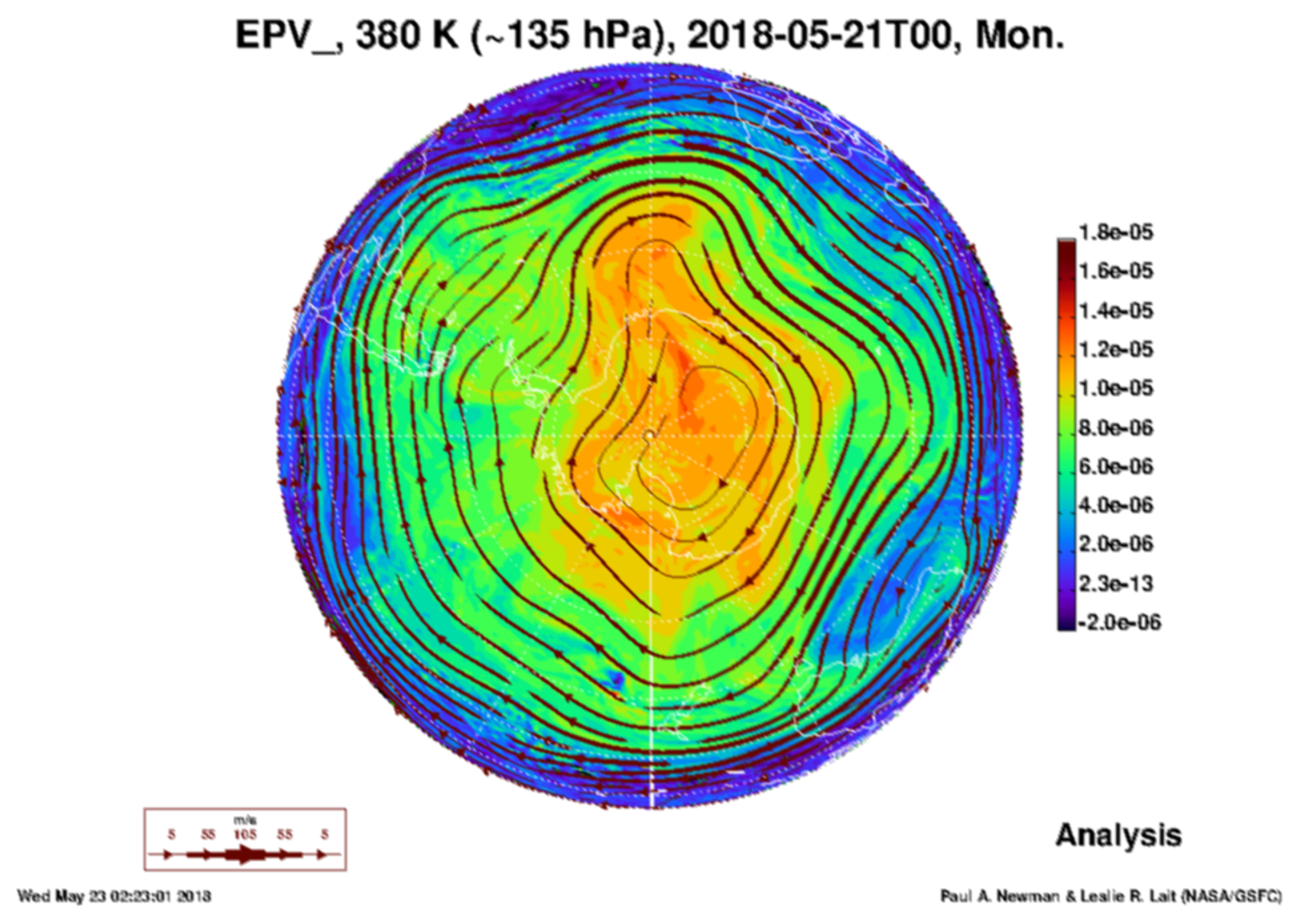
3.1. Antarctic Polar Vortex Phenomenon

The Antarctic polar vortex is a phenomenon that occurs in particular during winter season, where—due to earth’s rotation—a large mass of stratospheric air gets into a stable circular motion over several days to weeks.
The agents involved in this phenomenon are air parcels (the atmosphere over the Arctic). The rules are those basic fluid-mechanical rules described by the Navier-Stokes equations of fluid-dynamics: mass, momentum, energy conservation combined with an equation of state (e.g., ideal gas law). Additionally, these rules are formulated on a rotating manifold or sphere, as the earth is an almost spherical rotating planet. Therefore, the processes of geophysical fluid dynamics, a stratification of the atmosphere into layers like the stratosphere and the troposphere, mid-latitude westerlies, jet stream, etc. lead to a relatively stable circulation in the winter polar atmosphere, described for example in [13,14] .
The phenomenon can be described by the amount of Ertel’s (potential) vorticity. It is irrelevant which exact value needs to be chosen for the threshold constituting the vortex. However, this value can be computed from measured or simulated data and clearly distinguishes the vortex. An example is given in Figure 1.
In our mathematical notation, we can describe the phenomenon Antarctic Polar Vortex (APV) by
P APV = { v | P V v 1.0 × 10 5 K × m 2 k g s ; v unit volume ; P V v potential vorticity of v } .
Moreover, we can measure the size of the area covered by the Polar Vortex to establish a scale. We could also measure the time of occurrence. Or we could determine the total potential energy contained in the vortex. The Antarctic Polar Vortex in Figure 1 has a diameter of roughly 5500 km with an area covering approximately 112 × 10 6 km 2 .

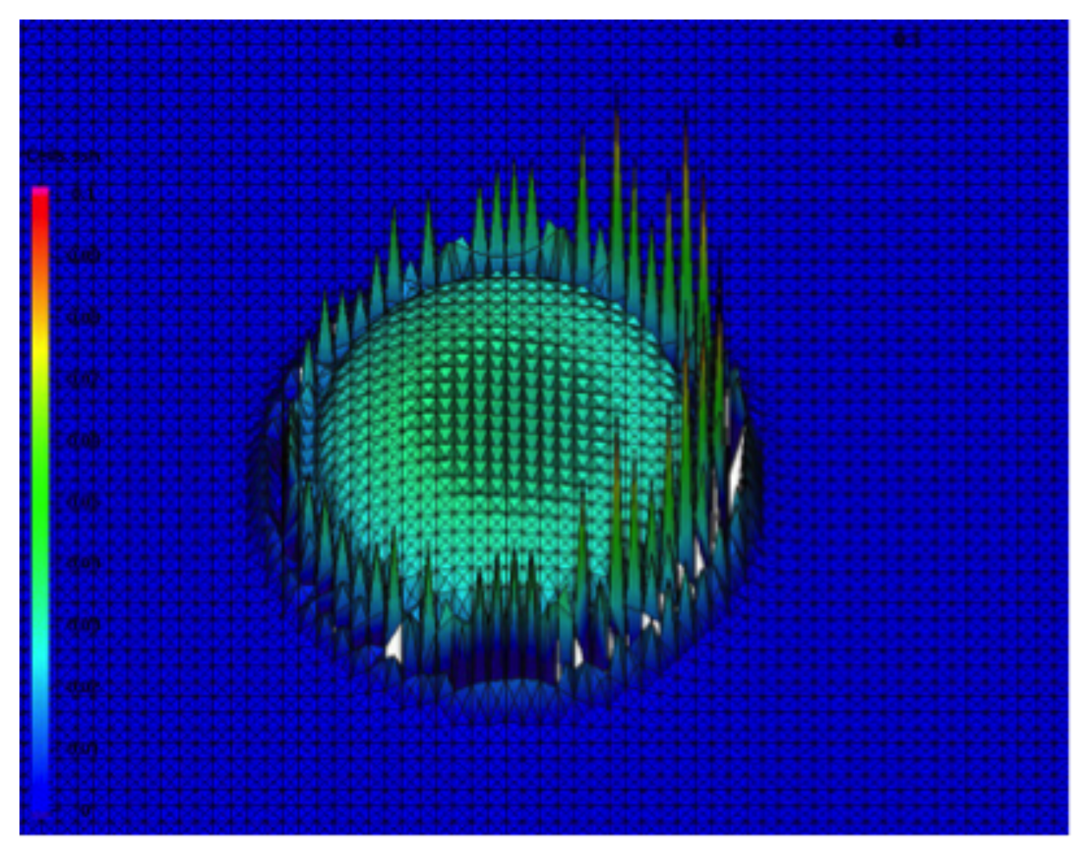
3.2. Unstable Numerical Model Phenomenon

While the description in the previous subsection was relatively straightforward and well established for a physical phenomenon, we want to apply the abstract concept to a non-standard phenomenon now. Unstable numerical methods often expose unphysical oscillations on a discretization grid size level (for details see [16]). An example of an unstable wave simulation is shown in Figure 2.
In this case, the agents are mathematical formulas, in particular maps for the time evolution, often denoted by a formula of the generic form
u ( t ) = E ( u ( t Δ t ) ) ,
where the function u : R + R d stands for the unknown time dependent state (e.g., the wave height of a propagating wave) that provides for each time t [ 0 , T ] R + a d-dimensional field describing the simulated state. E is an evolution that describes how u changes over time, in particular, how u ( t ) can be computed from a state u ( t Δ t ) at a previous time step ( Δ t being the time shift into the past).
The rules applied are established in E and are arithmetic operations, performed in floating point arithmetic (computers can only represent finite numbers of decimal digits, so real numbers are mapped to floating point numbers). Combined, these basic rules lead to time integration schemes for partial differential equations.
A numerically unstable scheme is characterized by the property that small perturbations (e.g., due to rounding error from real to floating point numbers) are amplified by the process E and grow over the integration time to render the solution useless (as demonstrated in Figure 2). The error of a numerical scheme can often be computed with respect to a known solution. Let u h be the numerical approximation to the true solution u, then the error can be written as e = | u u h | . Therefore, applying E to a small perturbation (or error) yields
e ( t ) = | u ( t ) u h ( t ) | = E ( | u ( t Δ t ) u h ( t Δ t ) | ) = E ( e ( t Δ t ) ) .
Now, if e ( t ) > e ( t Δ t ) , the algorithm is unstable. Therefore, assuming E a linear operator, representable as a matrix, the numerical scheme is unstable if for the spectral radius ρ ( E ) of E, i.e., the maximal eigenvalue of E, ρ ( E ) > 1 . So, again we have found a criterion or threshold to rigorously determine the phenomenon.
The scale of this phenomenon is hard to measure in spatial or time extend. Of course one could determine the number of time steps until a certain error threshold—given an initial perturbation size—is reached. However, since the model equations can be rescaled, an absolute value does not make sense at all. The spectral radius could be used to measure a scale of the phenomenon.

4. Discussion and Outlook

So far, we have introduced a notion of scales that is derived from relatively abstract and basic terms. This basic notation is intended to help communicate scales in the climate system across disciplines.
It is important to stress that this conceptual approach does not establish an analysis tool or a means to understand the internal mechanics of scales. It is a descriptive approach that is kept abstract, using the language of mathematics, in order to communicate without a disciplinary context.
This notation has demonstrated its usefulness in a course that has been taught for three consecutive summer terms within the master’s program “Integrated Climate System Sciences” at Universität Hamburg.
An interesting question was raised during these courses, namely whether the concept could also be used to describe scale interaction. A preliminary concept was developed, based on the idea of resonance effects, which will be outlined briefly in the following subsection. It should be noted that this concept is preliminary and—again—not intended to explain or analyze scale interactions but only to describe scale interaction in a discipline-independent language.

4.1. Interaction of Scales

As a motivation, we consider two examples of scale interaction:
  • El Niño Southern Oscillation (ENSO) is a phenomenon that occurs every five to ten years, characterized by a certain pattern of tropical Pacific sea surface temperature (see [17]). In principle the sea surface temperature in the tropical Pacific is oscillating with the seasonal cycle yielding warm surface waters in Summer and colder temperatures in Winter. Every now and then a strong anomaly in this pattern occurs such that the surface temperature in a large region is up to 3 C warmer than normal, triggering a whole cascade of subsequent processes commonly called the El Niño Phenomenon or El Niño Southern Oscillation (ENSO). As a side remark the reader may notice that this phenomenon is linked to the seasonal oscillation of sea surface temperature and therefore only occurs around November/December, a reason it is called el Niño—the Spanish expression for the (Christ) Child.
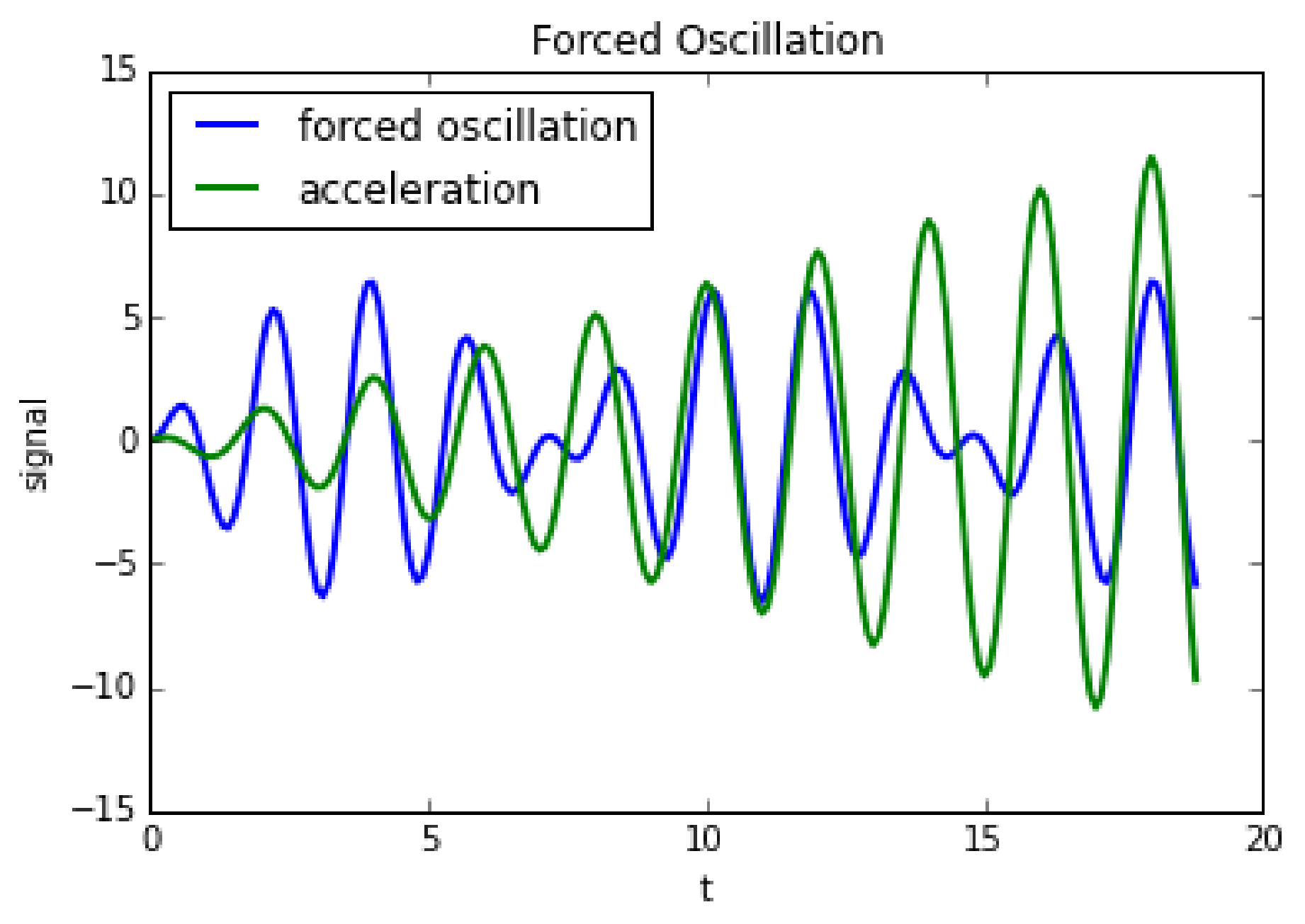
  • A children’s swing or rather the phenomenon of a swinging child is characterized by a child sitting on an especially designed pendulum, which is triggered by a deliberate movement of legs and arms of a child at the eigenfrequency of that pendulum. The child is swinging, if the pendulum deviates from its balanced state by a certain amount.
The above examples are characterized by a certain phenomenon, and processes that trigger this phenomenon. However, the processes triggering the phenomenon are of quite distinct size than the phenomenon itself. Seasonal cycling (i.e., the cycle through states related to spring-summer-autumn-winter) can be formulated as a phenomenon itself; it has a period of one year. The El Niño phenomenon is again a cyclic event, but with a less regular and less frequent occurrence. The swing’s movement and deviation from balanced state is triggered by inserting (at the right frequency) small amplitude/low energy momentum into the system. These observations motivate to utilize resonance phenomena as a role model for scale interaction.
A forced resonance is given by a differential equation that basically represents Newton’s second principle, i.e., force balances mass times acceleration. We mention the equation here for reference:
m x ¨ + c x ˙ + k x = F ( t )
We have used m as the mass of a body, x as its location, c as the damping factor (e.g., by friction), k the spring constant (we assume the body to be attached to a spring that tries to move it back into its original position), and F the forces acting on the body.
After some simplifications and algebraic modifications, we can express the solution as
x = C 1 cos ( ω 0 t ) + C 2 sin ( ω 0 t ) + F 0 ω 0 2 ω 2 cos ( ω t )
with ω 0 the eigen frequency of the system, C 1 and C 2 constants to be determined from the system parameters. So, the solution is a modulated wave. Depending on the system parameters, different behavior can be observed. We give two examples:
  • For m = 0.5 , k = 8 , and F 0 = 10 , and initial conditions x ( 0 ) = x ˙ ( 0 ) = 0 , we obtain the solution x = 20 16 π 2 ( cos ( ω t ) cos ( 4 t ) ) .
  • For m = 1 (normalized mass), k = ω 2 , and F 0 = F 0 m we obtain a system that is forced with its eigen frequency. In this case, the solution can be given as x = C 1 cos ( ω t ) + C 2 sin ( ω t ) + F 0 2 m ω t sin ( ω t ) .
The two solutions are visualized in Figure 3 in order to make the two regimes visible. For case 2. we assume C 1 = C 2 = 0 and m = 1 , F 0 = 2 , ω = π .
The two cases above demonstrate a typical behavior of resonances. The oscillation of the force on the right hand side interacts with the eigen frequency of the system. In the first case (1, Figure 3 blue line) the system has a different eigenfrequency compared to the frequency of the force. Therefore, the behavior of the forced system is somehow oscillatory, but stable. In the second case (2, Figure 3 green line) the force triggers an amplification of the system’s oscillation, because it acts in the same frequency. Eventually, the signal will be amplified to infinity, blowing up the solution.
These observations motivate us to propose the following formulation for scale interaction. First, we need to understand that the interaction of scales can only be initiated by processes. Processes drive the whole machine and lead to phenomena. Thus, phenomena can only be linked by processes. For simplicity, we will not distinguish between rules and processes at this point, since they both have the same effect modifying the agent’s state/attributes.
So, let us assume there are processes p 1 , p 2 , , p n that are to some extent relevant for two phenomena Φ 1 and Φ 2 . Then the total effect of those processes can be written as
p = k = 1 , , n C k p k .
Think of C k as the strengths and p k as the waves (as above). If the p k are triggered by a phenomenon Φ 1 then if p leads to a threshold above the definition level for phenomenon Φ 2 the first phenomenon can cause/trigger the second. In addition, this interaction establishes a scale interaction: the small-scale process of swinging legs, triggers the phenomenon of a swinging child.

4.2. Limitations

While the concept allows us to formulate several phenomena and processes stemming from diverse disciplines, it was found that the concept is based on several implicit assumptions
  • One assumption that was exposed during intense discussions in several interdisciplinary interactions is the reliance on quantifiable entities. This was felt to be a severe limitation by scholars representing a qualitative research direction in social sciences who could not cope with this approach.
  • A second cause for confusion was the inability of this approach to analyze or detect causalities. It is a purely descriptive approach. Therefore, the expectation that this formulation could reveal new knowledge about a multi-scale system is false.
  • A third implicit assumption that the notation in mathematical terms automatically clarifies confusion may not be true. The mathematically educated scholar may find the presentation not rigorous enough, while the non-mathematician may need a while to digest and understand the material. This is an experience taken from the courses taught on the topic of scales.

5. Conclusions

In this article, we introduced a formal approach to the notion of scales in the climate system. Despite some limitations it helps to communicate and use the concept of scales and scale interaction across disciplines. It is limited to those phenomena, being somehow quantifiable. However, the quantity measuring a scale cannot be uniquely determined, since phenomena can be defined in very diverse areas of research with similarly diverse defining quantities. The proposed notation allows for such diversity.
It is necessary to stress that the concept of scales does not (yet) provide a tool for deriving new insight into the structure of climate system related processes or phenomena. It is a descriptive language element to express such structure and interaction patterns, once they are known, observable, and measurable.
In [9] the notion of dynamical systems was utilized for an abstract definition of the term vulnerability. In fact, the dynamical system analogue could also be very powerful in describing the term scale. However, we decided to abstain from this analogy, because the theory of dynamical systems requires deeper mathematical insight with a lot more preparatory effort, such that understanding it is not straightforward for non-mathematicians.
With this abstract definition of scales in the climate system, we conducted several courses for interdisciplinary integrated climate system sciences students in Hamburg. The concept proved to be useful, though controversial, when applied to social sciences phenomena. Students could derive scale diagrams with this concept, which will be described in future publications. By choosing appropriate metrics, phenomena in different spheres (the natural sciences, social sciences, or economic sciences) can be related to each other.
With this concept we intend to contribute to a more rigorous understanding and theoretical basis for interdisciplinary climate research.

Funding

This research was funded by Deutsche Forschungsgemeinschaft (DFG) through the Cluster of Excellence CliSAP, grant number EXC177.

Acknowledgments

The author gratefully acknowledges input from students and co-lecturers of three courses on Scales in the Climate System taught in the School of Integrated Climate System Sciences (SICSS) at University of Hamburg, as part of CliSAP. Furthermore, the author is thankful for the fruitful discussion on this manuscript with Rupert Klein (FU Berlin). Finally, the anonymous reviewers with their constructive comments helped a lot to improve this manuscript.

Conflicts of Interest

The author declares no conflict of interest.

References

  1. Encyclopaedia Britannica. Climate—Scale Classes, Contributor Smith, P.J. Available online: https://www.britannica.com/science/climate-meteorology/Scale-classes (accessed on 10 June 2018).
  2. Adger, W.N.; Arnell, N.W.; Tompkins, E.L. Successful adaptation to climate change across scales. Glob. Environ. Chang. 2005, 15, 77–86. [Google Scholar] [CrossRef]
  3. Meehl, G.A.; Lukas, R.; Kiladis, G.N.; Weickmann, K.M.; Matthews, A.J.; Wheeler, M. A conceptual framework for time and space scale interactions in the climate system. Clim. Dyn. 2001, 17, 753–775. [Google Scholar] [CrossRef]
  4. Matthews, A.J. A multiscale framework for the origin and variability of the South Pacific Convergence Zone. Q. J. R. Meteorol. Soc. 2012, 138, 1165–1178. [Google Scholar] [CrossRef] [Green Version]
  5. Emanuel, K.A. On the dynamical definition(s) of “mesoscale”. In Mesoscale Meteorology—Theories, Observations, and Models; Lilly, D.K., Gal-Chen, T., Eds.; NATO ASI Series, Series C, Mathematical and Physical Sciences; Springer: Dordrecht, The Netherlands, 1982; Volume 114. [Google Scholar]
  6. Hurrell, J.; Meehl, G.A.; Bader, D.; Delworth, T.L.; Kirtman, B.; Wielicki, B. A Unified Modeling Approach to Climate System Prediction. Bull. Am. Meteor. Soc. 2009, 90, 1819–1832. [Google Scholar] [CrossRef] [Green Version]
  7. Lovejoy, S.; Crucifix, M.; de Vernal, A. Scale and Scaling in the Climate System. Pag. Mag. 2016, 24, 33. [Google Scholar] [CrossRef]
  8. Pasini, A.; Lorè, M.; Ameli, F. Neural Network Modelling for the Analysis of Forcings/Temperatures Relationships at Different Scales in the Climate System. Ecol. Model. 2006, 191, 58–67. [Google Scholar] [CrossRef]
  9. Ionescu, C.; Klein, R.J.T.; Hinkel, J.; Kavi Kumar, K.S.; Klein, R. Towards a Formal Framework of Vulnerability to Climate Change. Environ. Model. Assess. 2009, 14, 1–16. [Google Scholar] [CrossRef]
  10. SICSS. School of Integrated Climate System Sciences—Homepage. Available online: http://www.sicss.de (accessed on 10 June 2018).
  11. Baehr, J.; Behrens, J.; Brüggemann, M.; Frisius, T.; Glessmer, M.S.; Hartmann, J.; Hense, I.; Kaleschke, L.; Kutzbach, L.; Rödder, S.; et al. Teaching Scales in the Climate System: An example of interdisciplinary teaching and learning. Geophys. Res. Abstr. 2016, 18, EGU2016-10680. [Google Scholar]
  12. Looney, D.; Hemakom, A.; Mandic, D.P. Intrinsic Multi-Scale Analysis: A Multi-Variate Empirical Mode Decomposition Framework. Proc. R. Soc. A 2015, 471, 20140709. [Google Scholar] [CrossRef] [PubMed]
  13. Vallis, G.J. Atmospheric and Oceanic Fluid Dynamics; Cambridge University Press: Cambridge, UK, 2006. [Google Scholar]
  14. Waugh, D.W.; Sobel, A.H.; Polvani, L.M. What is the Polar Vortex and How does it Influence Weather? Bull. Am. Meteor. Soc. 2017, 98, 37–44. [Google Scholar] [CrossRef]
  15. Newmann, P.A. GSFC Meteorological Plots for the Antarctic—GMAO GEOS 5.7 products. Available online: https://acd-ext.gsfc.nasa.gov/Data_services/Current/antarctic/index.html (accessed on 10 June 2018).
  16. Higham, N.J. Accuracy and Stability of Numerical Algorithms; SIAM: Philadelphia, PA, USA, 2002. [Google Scholar]
  17. Trenberth, K.E. The Definition of El Niño. Bull. Am. Meteor. Soc. 1997, 78, 2771–2777. [Google Scholar] [CrossRef] [Green Version]
Figure 1. Ertel’s potential vorticity (EPV) generated from analyzed wind data at the 380 K potential temperature level, i.e., in the Antarctic stratosphere at approximately 14 km altitude. Plot shows EPV on 21 May 2018, in units of K × m 2 k g s (see [15]).
Geosciences 08 00213 g001
Figure 2. Instabilities at the wave front exposed by an unstable numerical scheme for wave propagation. The spurious peaks in the numerical solution are of the size of the grid cells (shown as triangles). The colors indicate wave height above mean water level. The plot shows one snapshot of a shallow water wave propagation simulation.
Geosciences 08 00213 g002
Figure 3. Two different regimes of a forced oscillation. Blue: scale interaction without amplification; green: amplification of amplitude.
Geosciences 08 00213 g003

