Article

The Impact of Acoustic Imaging Geometry on the Fidelity of Seabed Bathymetric Models

by
John E. Hughes Clarke
Center for Coastal and Ocean Mapping/National Oceanic and Atmospheric Administration (NOAA) Joint Hydrographic Center, University of New Hampshire, Durham, NH 03824, USA
Geosciences 2018, 8(4), 109; https://doi.org/10.3390/geosciences8040109
Submission received: 4 March 2018 / Revised: 20 March 2018 / Accepted: 22 March 2018 / Published: 24 March 2018
(This article belongs to the Special Issue Marine Geomorphometry)

Abstract

:
Attributes derived from digital bathymetric models (DBM) are a powerful means of analyzing seabed characteristics. Those models however are inherently constrained by the method of seabed sampling. Most bathymetric models are derived by collating a number of discrete corridors of multibeam sonar data. Within each corridor the data are collected over a wide range of distances, azimuths and elevation angles and thus the quality varies significantly. That variability therefore becomes imprinted into the DBM. Subsequent users of the DBM, unfamiliar with the original acquisition geometry, may potentially misinterpret such variability as attributes of the seabed. This paper examines the impact on accuracy and resolution of the resultant derived model as a function of the imaging geometry. This can be broken down into the range, angle, azimuth, density and overlap attributes. These attributes in turn are impacted by the sonar configuration including beam widths, beam spacing, bottom detection algorithms, stabilization strategies, platform speed and stability. Superimposed over the imaging geometry are residual effects due to imperfect integration of ancillary sensors. As the platform (normally a surface vessel), is moving with characteristic motions resulting from the ocean wave spectrum, periodic residuals in the seafloor can become imprinted that may again be misinterpreted as geomorphological information.

1. Introduction

Geomorphometry is a mature field in terrestrial sciences but is less well known in the marine realm. While the concepts were applied to multibeam data several decades ago [1,2,3,4], only now, with the easier availability of GIS tools, are they routinely being applied toward seabed topographic applications (a comprehensive review can be found in [5]). As with the terrestrial terrain measurements, those parameters extracted from a digital bathymetric model (DBM) are ultimately limited by the quality of the original observations. This paper focuses on the achievable spatial resolution of the most widespread seafloor bathymetric survey instrument used: Integrated multibeam sonar systems.
This paper is part of a special edition of Geosciences devoted to marine geomorphometry. The other papers [6,7,8,9,10] present specific applications, predominately utilizing multibeam sonar observations. The scales of features investigated vary by two orders of magnitudes including deep-water (2000–5200 m) observations [6,7], outer shelf (135–376 m) [8], and shallow (10–50 m) water [9,10,11]. For all cases, the features of interest range from 0.2 to 10% of the total water depth in the vertical and 2–20% of the elevation in the horizontal. The lower end of these dimensions approaches the limits commonly achievable by these sonar systems. As such, artefacts specific to the acoustic imaging geometry, can be developed in the data at the same scale as the morphologic features of interest.
This paper is arranged to first introduce the multibeam sonar geometry and then explain the controls on achievable resolution as a function of a wide variety of parameters. A particular focus is provided for those system artefacts that are developed close to the limit of the achievable resolution. This is because, as noted by several researches [5,12], the seafloor geomorphic features of interest are often at, or close to, the limit of achievable resolution and are thus prone to potential distortion.
Each aspect discussed is illustrated by specific example data so that the reader may recognize the net result in a derived terrain model. Specific formulas to attempt to calculate solution density are omitted as they are strongly dependent on sonar configurations and motion history which are continuously variable and rarely stored with derived gridded products.

2. Multibeam Imaging Geometry

A multibeam echosounder is an acoustic scanner that delivers sequential topographic profiles aligned approximately orthogonal to the platform (a surface or submerged vehicle) trajectory. It does this by taking advantage of the Mills Cross array geometry to ensonify a corridor and then receiving the backscattered energy through a number of discrete beamformed channels at a variety of elevation angles [13,14]. As the vehicle advances, successive profile solutions build up a swath corridor. Different sonar models utilize different beam dimensions, spacings and density. As these sonar systems operate predominantly from underway platforms, they vary in their approach to stabilization in order to compensate for motions primarily within the ocean wave spectrum. It is those resultant data that are the underlying input to digital bathymetric models (DBM). Two primary, but quite separate, factors concerning the input data will become apparent in this discussion: The solution density, and the achievable resolution based on the footprint within which a single solution in derived.
Were those swaths of data made up of evenly spaced solutions, each of which represented the depth from an identically sized footprint, the data might be expected to be equivalent. In reality, however, as the vehicle does not follow a straight line path and rotates on three axes (roll, pitch and yaw), the solution density is uneven. Furthermore, the ensonified area, defined by the product of the transmission and receiver patterns (and/or pulse duration and processing), is not of uniform size and the incidence angle of acoustic energy is highly variable. As a result, both the solution density and the solution resolution vary strongly with both elevation and across a single swath. These factors will impact the resolved terrain roughness thereby affecting any classification scheme based on surface characteristics.
The closest analogous instrument used for terrestrial surveying is an airborne laser scanner (ALS). To contrast a multibeam sonar to an ALS, the geometric differences need to be appreciated (Figure 1).
The laser scanner sector elevation angle is typically only varying from vertical to ~20–25° incidence angle. For a typical ALS, the projected laser beam divergence is on the order of ~1 millradian (0.0573°) [15]. At a flying height of ~550 m this has a footprint then of 0.55 m at nadir growing to only 0.64 m at the edge of the swath. As the flying height is normally much larger than the variation in elevation of the feature of interest (e.g., examining rock ridges of ±20 m scale), the beam footprint only varies by ±3–4% as a result of within swath surface elevation fluctuations. For larger scale terrain fluctuations that occur over longer wavelengths, the aircraft is free to adjust its vertical trajectory to maintain a similar altitude.
In contrast, a good multibeam has a beam width of typically 1° (qualifications on this will be discussed later), but projected over an angular sector of up to ±65°. For a continental shelf depth of 50 m, this results in footprints ranging from 0.87 m at nadir to 2.1 m (along) or 4.9 m (across-track) at the edge of the swath. Additionally, for the case of within swath topography that varies within the same range (±20 m), those dimensions fluctuate by up to 40%.
The preceding simplified geometric scaling calculations demonstrate that variations in the effective resolution are going to be much more pronounced across a multibeam swath than an ALS swath. Even with the reduced changes, the variation in the ALS footprint is known to have an impact in the effective data quality [16]. Such effects are thus magnified for the multibeam geometry which, in turn, will impact the achievable terrain discrimination using geomorphometric techniques.

3. Component Contributors to Resolution Limits

Given the grossly different scale of imaging geometry discussed, the components that influence the multibeam imaging geometry are now broken down and described separately. Specific real examples are provided where that change in the component influences the appearance of a morphologic feature that might be of interest.

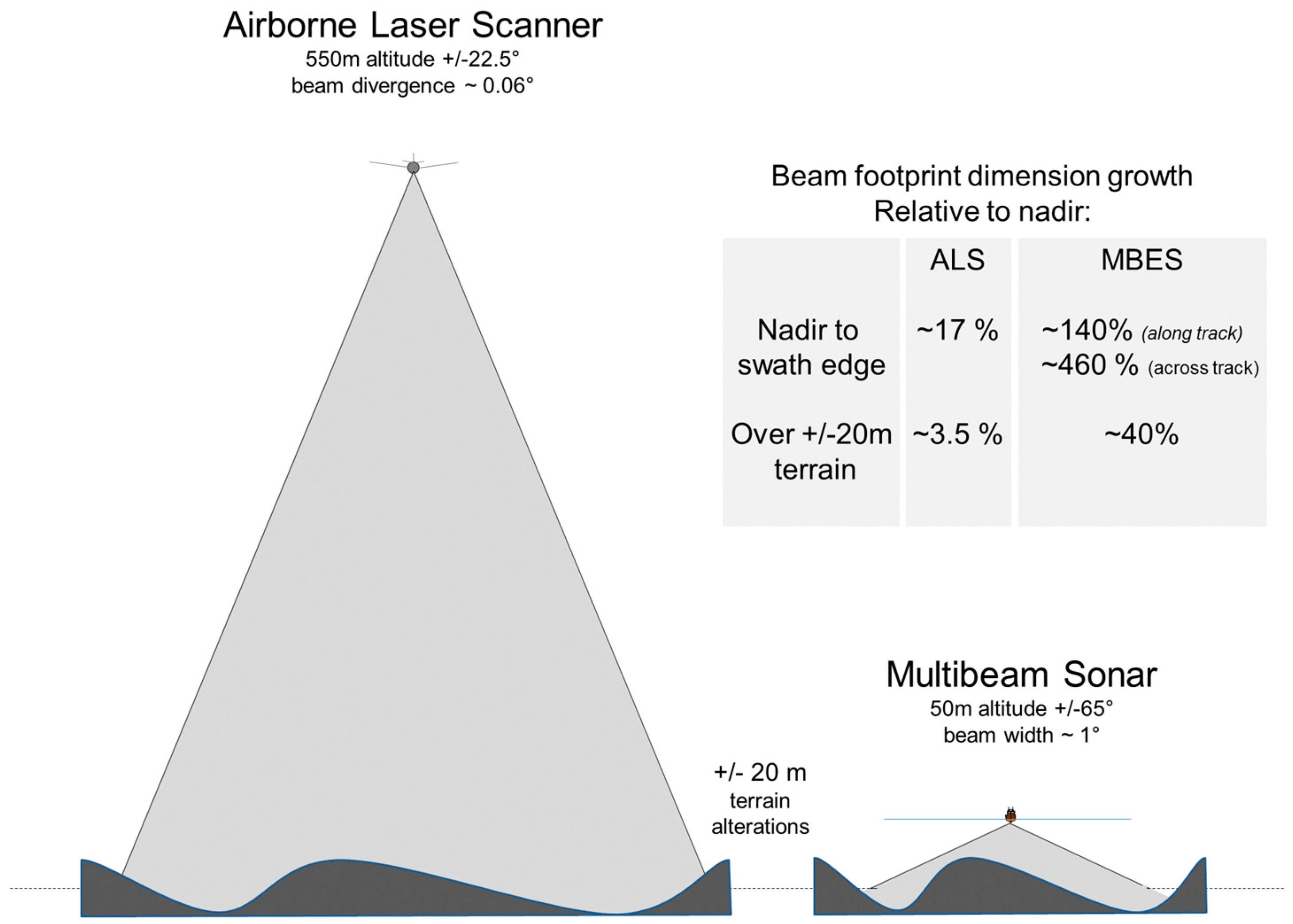
3.1. Projected Beam Width Aspects

For a singular beam bottom detection, the range solution is constrained to be from within an area on the seafloor that lies within the projected beam dimension. That in turn reflects the beam widths of the transmitter and receiver respectively. Those are controlled by the array dimensions in wavelengths and the shading applied. Typical quoted beams widths range from 0.5 to 2.0 degrees and are often not the same for transmit and receive (thus the footprint for normal incidence is already elliptical). Figure 2a–d illustrate the loss in feature definition for the same target with differing Tx and Rx beam widths. If a critical geomorphic parameter is the presence of short wavelength targets such as boulder fields (a common habitat indicator), their visibility will strongly depend on the specific sonar beam width, and vary with elevation and obliquity.

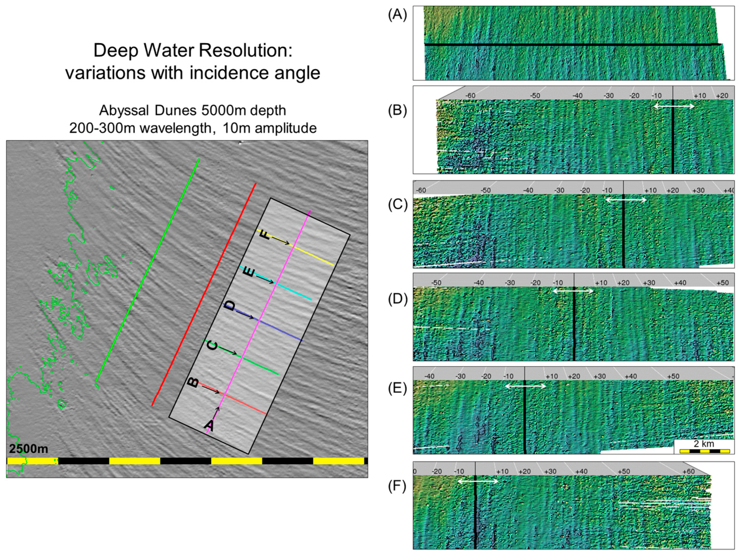
3.1.1. Steering, Range, Obliquity and Seafloor Slope
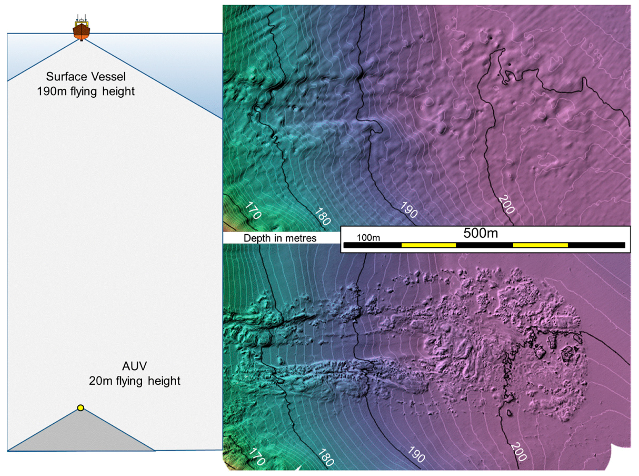
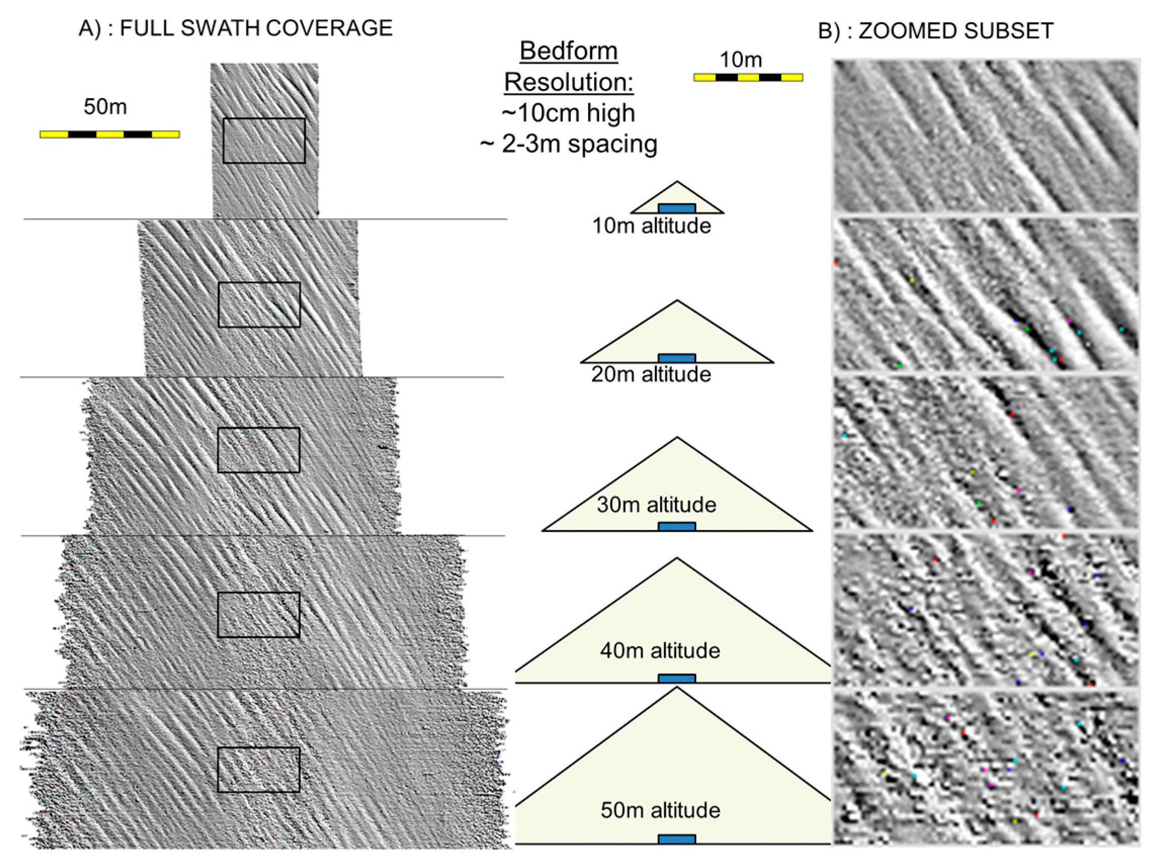
For any quoted beam width the nominal value reported in the specifications is only true when unsteered. A typical multibeam system (level receiver) will steer on receive more than 60° to achieve the across-track coverage. The steered receiver beam width is correspondingly expanded (×2 for 60° ×4 for ~75°). That beam is then projected over the slant range onto an increasingly oblique seafloor incidence. The net result, for a level receiver and a flat seafloor, is a ~1/cos3 (steering angle) dependence on the across-track dimension and a 1/cos dependence for the along-track dimension. This of course is modulated by the local seafloor slope, with poorer definition on seafloors tilted away from the beam vector.
This elongation would rapidly become detrimental if the range estimation were purely defined from center-of-mass type algorithms (as is the norm for ALS). To ameliorate that effect, almost all multibeam systems use a split aperture approach [17] to estimate the geometric center of the beam in the across-track direction (phase detection, see Section 3.2.1). Unlike fisheries sonars however, the split aperture is only applied across-track and thus the along-track dimension (the projection of the transmit beam) remains a constraining limit on resolution (thus only a 1/cosine dependence) [18].

3.1.2. Elevation

Unlike airborne scanners in which the vehicle is free to alter its altitude above the terrain to optimize the solution density, a surface-mounted multibeam is forced to accept the altitude change as the topography rises and falls. If the roughness characteristic of interest is close to the resolution limit, then the feature may be distorted or even disappear with increasing depth.
Unlike surface mounted systems, however, the increasing use of autonomous underwater vehicles (AUVs) allows the decoupling of the resolution from the depth. Figure 3 illustrates the impact of altitude on feature resolution.
An additional benefit of AUV operations is that the altitude can be adjusted to trade-off required resolution versus coverage. Figure 4 illustrates the achieved definition of short wavelength roughness targets (flutes) as a function of elevation. Notably, even before the real relief is lost, the impact of noise due to the bottom detection method (see Section 3.2), starts to appear and can be confused with shorter wavelength relief. Again this will impact the morphometric parameters extracted from the terrain leading potentially to a false classification.

3.2. Bottom Detection Effects

For a single receiver channel, the intensity time series received from the location at which the main lobe of the beam strikes the bottom represents a finite time interval. That duration is strongly dependent on the beam dimension and the obliquity as discussed in Section 3.1.1. Depending on the elongation of the echo envelope two main bottom detection algorithms (amplitude and phase) are employed [17,19]. Both vary in their resulting quality of range estimation as a function of incidence angle. As a single swath sweeps through the full range of incidence angles and systematically switches from one to the other bottom detection method, the noise characteristics of each bottom detection algorithm become embedded in the swath sounding corridor in a systematic manner. Unless this is recognized, the resultant varying seafloor rugosity can be confused with a real seafloor morphometric change.

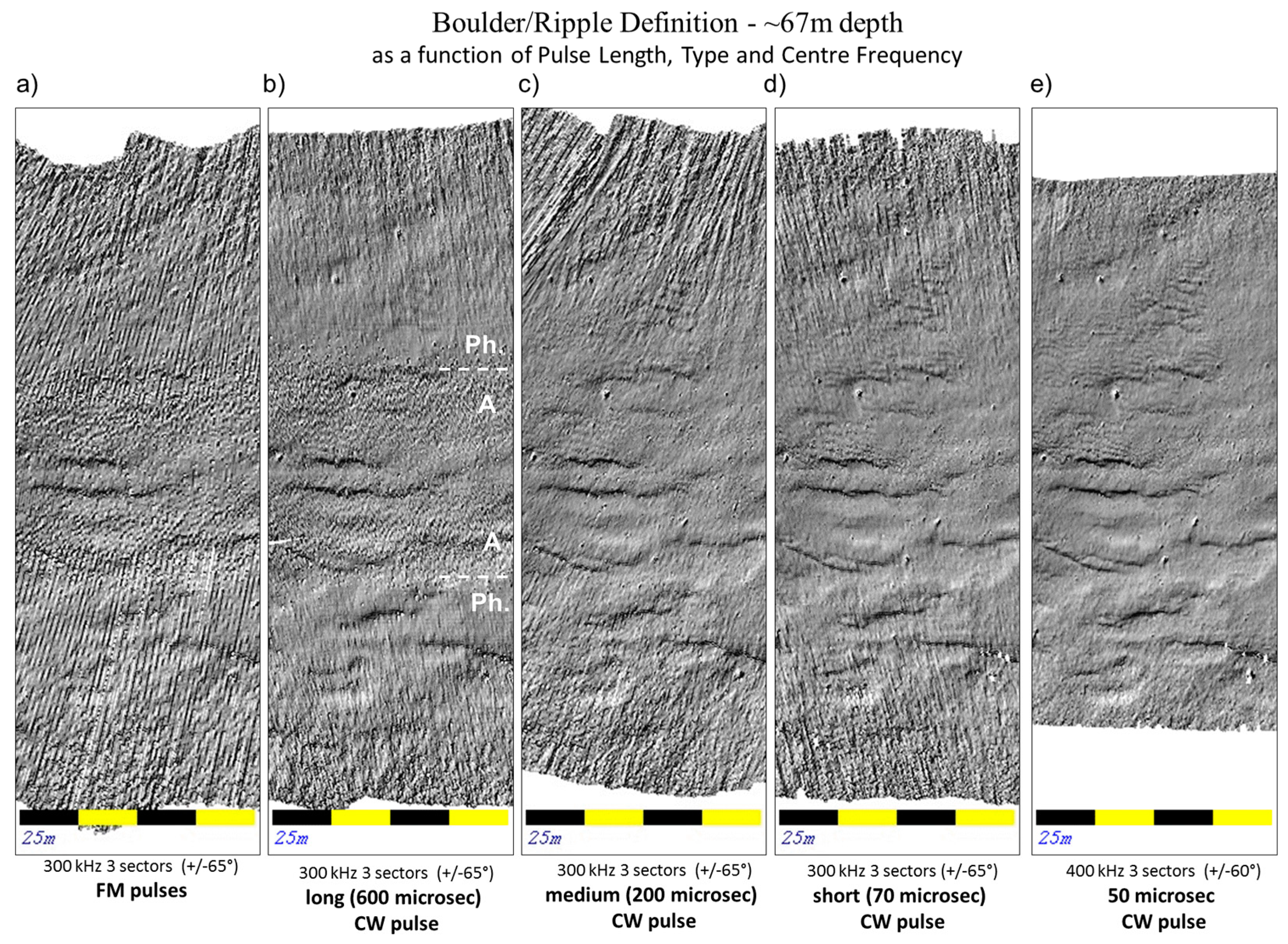
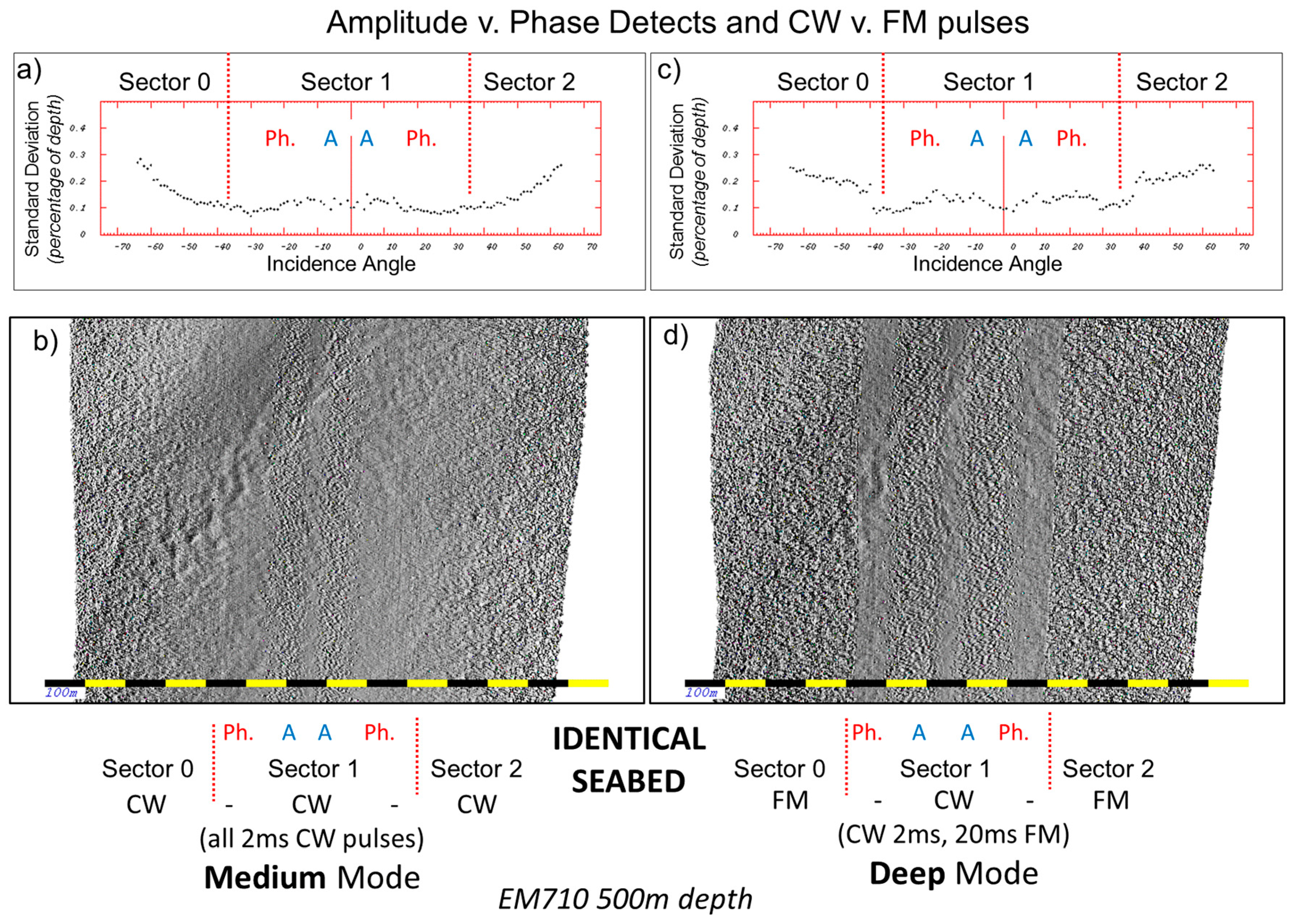
3.2.1. Amplitude vs. Phase Detection

The two common approaches employed to identify the location of the center of the beam within the received echo envelope are amplitude and phase detection. Details on the algorithmic approach can be found in [17,19]. The amplitude method relies heavily on the length of the echo envelope, and is thus optimal for the near normal incidence methods. As the angle of incidence (AOI) becomes more oblique, the range estimation can be increasingly biased towards hotspots in backscatter strength within the beam footprint. This manifests as apparent random noise in the range estimation that grows rapidly with obliquity.
In contrast, the phase estimation uses a split aperture approach and is thus relative insensitive to variations in the seabed backscatter strength within the beam footprint. As a result, for an AOI at which both bottom detection methods can be employed, the phase detection will generally be lower noise. As a result when the system switches between the two range estimation methods, there is often a characteristic change in the apparent roughness of the seafloor at that location (Figure 5 edge of white arrows).
Unlike the amplitude detection approach, the phase detection need not utilize all the information across the wide across-track beam footprint. As long as the signal to noise ratio is high enough, the phase detection zero crossing may be based on fewer phase samples and thus relief across-track at scales significantly smaller than the projected beam footprint are possible [18]. Thus, the apparent scaling by projected beam footprint, presented in Figure 1 is not so pronounced.
At the outer limits of the swath, as the signal to noise ratio reduces, the phase detection algorithm gradually gets less accurate and there is a corresponding increase in the sounding noise again (Figure 5, outer edges of swaths in B and F).
Figure 5 illustrates this phenomena, showing abyssal dunes that have a distinct morphometric signature. As can be seen, the appearance of the same dune at differing grazing angles is inconsistent in its apparent rugosity and thus might be classed as slightly different geomorphic character. The only way to remove this differential bottom detection noise would be to grid the data as a scale that suppresses this beam-to-beam uncorrelated noise, although this could then partially obscure the feature of interest.

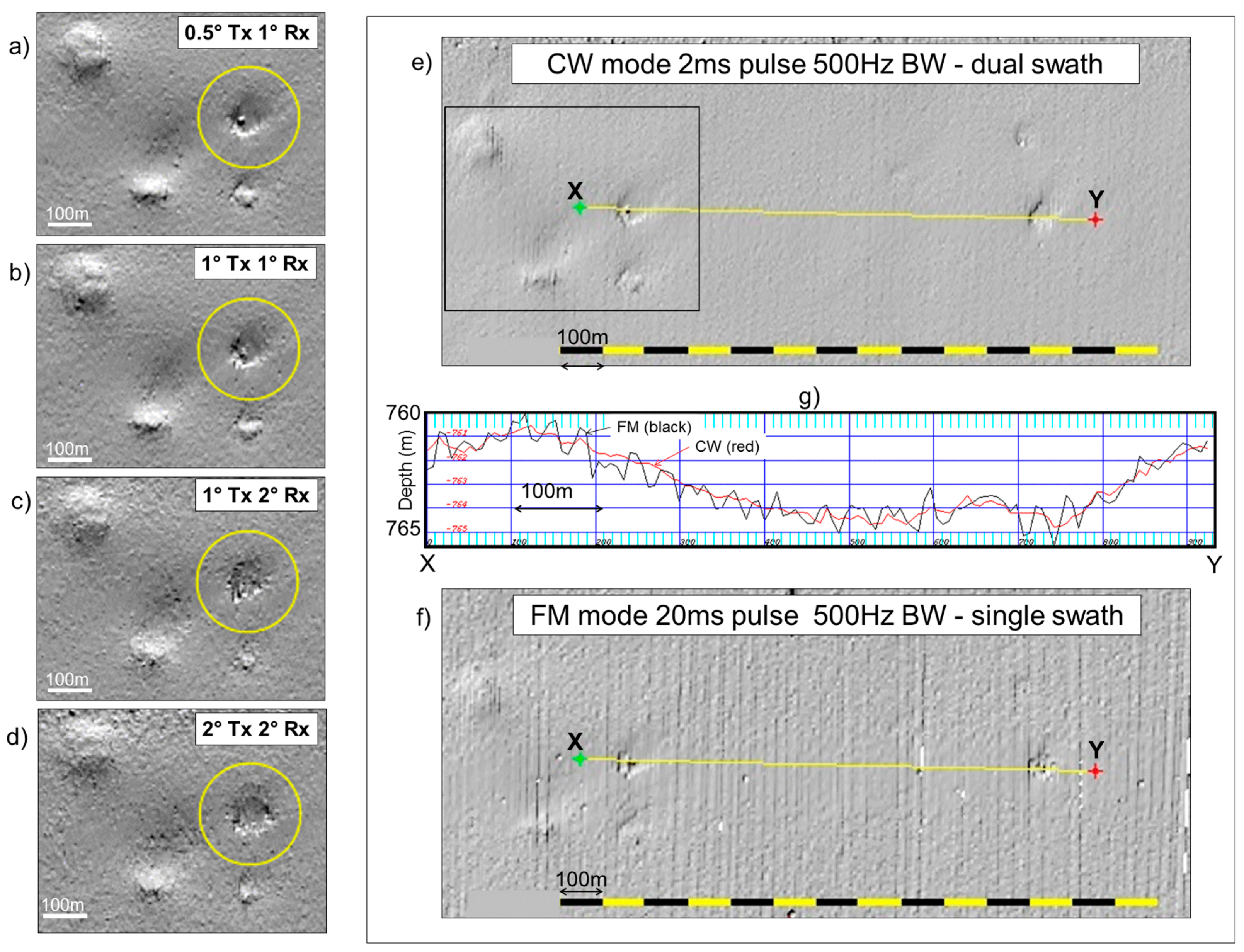
3.2.2. FM vs. CW Pulses

For a subset of the available multibeam systems on the market, the benefits of pulse compression are being employed to increase the range performance. Most commonly, linear frequency modulated (LFM) pulses are being employed that increase the signal to noise. While the range performance improves there are three complications that impact the appearance of low relief seafloors that could be confused with real rugosity.
  • The first is a result of the Doppler heave distortion of the pulse [20].
  • The second is the loss of the dual swath capability due to duty-cycle limitations.
  • The third is a result of the imperfection of the matched filter process [21].
All three effects will alter the short wavelength attributes of a derived DBM and thus could confound geomorphic analysis.
Figure 2e–g illustrates the combined first two effects. The extracted seafloor profiles (Figure 2g, X-Y) of the same terrain are only corrugated when the FM pulse is used. This is a result of the Doppler heave effect where the array motions at transmit and receive distort both the outgoing and incoming LFM pulse and result in a small time shift in the matched filter process [20]. The example shown has not correctly had the shift accounted for (this correction is now routinely applied). Note the scale of this artefact, 0.7 m in 700+ m of water, a ~0.1% of depth anomaly. Even though this is a small effect it is of the same order as the small targets (see Figure 2a–d) that the sonar is being used to resolve.
The second LFM-related effect manifests as a result of the fact that the sonar system involved (EM710) normally utilizes a dual swath strategy (see Section 3.3.3) using 3 sectors per swath. A total of 6 × 3 ms pulse (18 ms total transmission time) are required for continuous wave (CW) pulse operation in the depths considered. For the LFM configuration, a single swath now utilizes 2 × 40 ms and one 20 ms pulse (a total of 100 ms). A second transmission cannot be employed as the duty cycle of the transmitter would be exceeded. The net result is the along-track data density is now half that of the CW mode. This accentuates the visibility of the Doppler heave artefact.
For the case of multi-sector systems (see Section 3.3.2) which are able to employ differing pulse types in each sector, often the central sectors utilize CW pulses whereas the outer sectors switch to LFM pulses to maintain signal to noise. The net result is that the bottom detection noise in notably different. Figure 6 illustrates the higher noise evident when the equivalent bandwidth FM pulse is substituted instead of a CW pulse for the outer sectors. With these mixed pulse type modes, dual swath is maintained and the FM pulse has the same bandwidth so the noise would be expected to be similar. Comparing Figure 6b,d, however, this is clearly not the case as an abrupt jump in the surface roughness is apparent at the CW-FM sector boundary. The sounding noise statistics jump up by a factor of 2 (Figure 6c). This effect is believed to be due to matched filter sidelobes [21]. It should be noted that this noise is at the 0.2% of depth (Z) level (one standard deviation) and thus is well within standard hydrographic performance specifications (~±1.3% Z). Although this is a small effect, it is at the same scale as genuine low relief sedimentary structures such as bedforms or depressions (such as developed on the left side of the swath in Figure 6b) and thus potentially can confuse geomorphic analysis. This particular sonar system switches automatically between these two modes at about 500 m, so this spatially coherent noise contribution would abruptly appear and disappear within a DBM, potentially producing spatially varying rugosity unrelated to real seafloor characteristics.

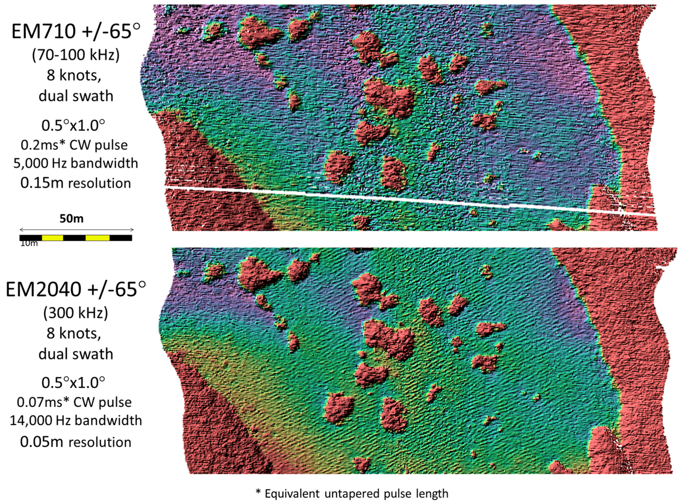
3.2.3. Pulse Length Changes

In order for a surface mounted multibeam to be able to cope with range dependent attenuation that changes continuously with water depth, it must alter its configuration to maintain adequate signal to noise. Almost all systems are operating at full power so usually the only means of adapting is to alter the outgoing pulse. A lengthening of the pulse provides both larger ensonified area (thereby increasing the bottom target strength) and, for the case of a CW pulse, a narrower bandwidth thus allowing better noise suppression. Such a switch, however, compromises range resolution which in turn impacts feature definition. Figure 7 illustrates two simultaneous views of the identical seafloor using two sonars with identical beam widths but different pulse lengths. The data were collected from co-mounted sonars on the same vessel so they share exactly the identical motion history and sound speed environment.
Pulse length changes are usually implemented as an abrupt and discrete shift in the sonar configuration (often referred to as modes, consisting of a new set of pulse lengths, receiver bandwidths and potentially beam spacing and angular sector). If the system is operating in automatic mode, the location and timing of such shifts are driven primarily by depth. Thus, within a derived DBM, abrupt changes in the achievable resolution may be visible, implemented as the survey tracks go up and down through a critical depth threshold.
The operator may disable such automated changes. Doing so, however, risks other data quality issues (such as poor signal to noise in deeper water). If, however, the depth ranges are small, then the operator may take advantage of better range resolution (potentially thereby accepting a narrow swath) if it is important to maintain definition of a critical seabed roughness element that can be used in geomorphometric analysis (see Section 3.2.2).
This issue of altitude-dependent resolution is of course of less concern for AUVs, which usually operate in terrain-following mode. The flying height can be pre-selected to maintain the required resolution (as illustrated in Figure 4).

3.2.4. Impact of Operator Selection of Pulse Lengths

Given the trade-offs between range performance and bottom detection noise, if the operator is interested in seafloor roughness at the limit of the system resolution, the choice of operating setting can influence the visibility of the target of interest. Figure 8 illustrates the appearance of smaller dunes, developed on the back of larger ones as a function of settings for the same sonar system.
Several aspects, including those previously discussed, are visible as the five different modes are utilized in turn. For the FM pulse (Figure 8a), the impact of loss of dual swath is evident. For the longest CW pulse (Figure 8b) the amplitude phase boundary is evident and only switches at about 20° incidence angle. As the pulse is shortened (Figure 8c), the switchover from amplitude to phase moves in and the noise associated with the amplitude detection is reduced. At the same time however, the loss of signal to environmental noise in evident in the outer part of the swath. Additionally, part of the apparent outer swath noise in Figure 5C,D is manifested as apparent across-track ribbing related to integration and will be explained in Section 3.5 and Section 3.6.
As the pulse is again shortened (Figure 8d), the visibility of a population of a smaller dunes superimposed on the back of the larger dunes increases. Finally, by switching to a slightly higher frequency (Figure 8e), with the corresponding narrowing of the beams, the best view is obtained, although at the expense of swath width.
If common geomorphometric parameters were extracted from each of these seafloor realizations in turn, the same seafloor could potentially be classified differently.

3.3. Beam Density Considerations
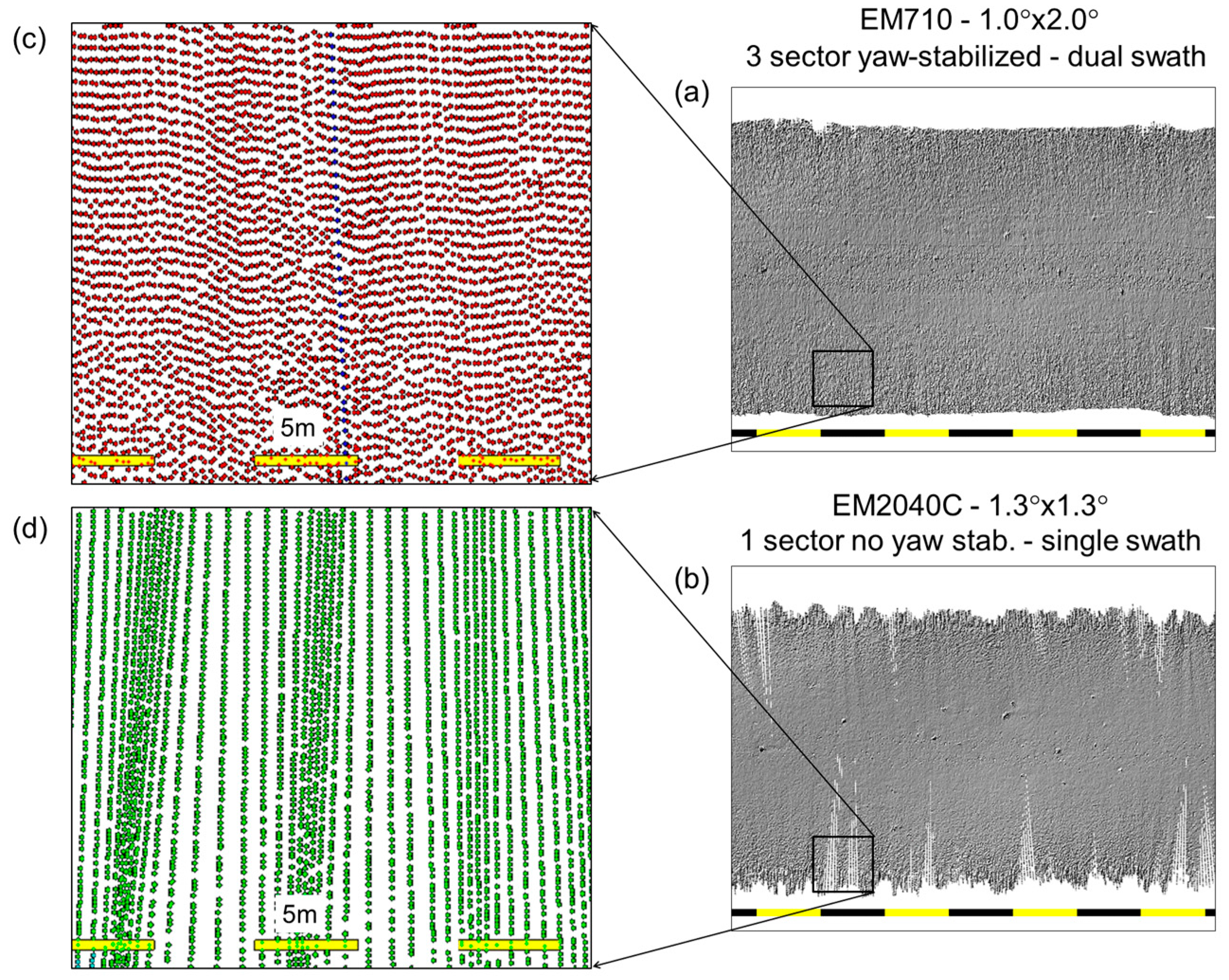
For a given pulse length and bottom detection strategy, the full benefit of the achievable resolution is only gained if the solution density is significantly tighter than the projected beam footprint. The beam density is not a constant however. Vessel speed, angular sector selected, stabilization strategy and availability of multi-swath are the main factors that influence this.
In the absence of sufficient solution density, the visibility of the shortest potentially-resolvable features can be compromised.

3.3.1. Beam Spacing

In the 1990’s it was common for multibeam systems to have an across-track beam spacing that was only as tight as the 3 dB beam width limit. Since then, increases in the available number of beam forming channels, together with the ability to dynamically adjust their spacing as the total angular sector is changed, has allowed tighter beam density (commonly to at least less than ½ of the beam width). These aspects manifest in both the across and along-track density.
With heavily overlapping beam footprints in the across-track dimension, the bottom detection solution from beam to beam shares much of the same signal and is thus no longer fully independent. Nevertheless, uncorrelated noise contributions between individual bottom detections will be suppressed in an oversampled situation. Thus reducing the angular sector, thereby producing higher across-track solution density, will suppress sounding noise and promote the visibility of true short wavelength seabed relief.
As a byproduct of reducing the angular sector, the two-way travel time (twtt) to the outermost beam is reduced. As a result, the ping rate of the system is normally allowed to increase (typical ping rates are about 1.2 × this twtt). Thus reducing the angular sector also benefits the along-track solution spacing. For common operating speeds of ~8 knots (4 m/s), a ±65° swath will result in the along-track solution density being ~1.5% of depth. This is only about the 3 dB dimension (for a 1° Tx) and thus there is minimal along-track oversampling. If, however, the sector is compressed to ~±25° (e.g., Figure 5A) the swath width is reduced by a factor of 4.6 and the twtt by 2.1, resulting in ~10 × the sounding density resulting in better definition than the wider sector (Figure 5B–F).
For most surface mounted multibeam systems, the along-track density is generally the more critical limiting factor (e.g., Figure 9d). Furthermore this simplified calculation ignores the additional complication for the along-track data density of azimuth and pitch rotations of the survey platform from ping to ping.

3.3.2. Stabilization, Pitch and Heading

The preceding along-track data density calculations ignored both pitch and yaw perturbations. Pitch perturbations displace successive swaths along-track and yaw perturbations can dramatically degrade the along-track density on the outer side of a turn.
To address this, multi-sector yaw stabilization is now available that breaks the swath into sub sectors across-track and drastically reduces the impact of yaw and pitch on the along-track solution density [22].
Figure 9 illustrates the impact of having multi-sector stabilization. The two examples were acquired simultaneously from two systems mounted on the same vessel operating in open water. Both systems were operating with the same angular sector (±65°) and the same ping rate (synchronized). The scale of the yaw motion was ~±2° over ~10 s and the pitching was up to ±2° in 4 s. As can be seen, the sounding density is very uneven for the single sector system (Figure 9d) and thus compromised with potential data gaps larger than 1m. In this water depth, both those systems are capable of resolving 1 m targets if sufficient sounding solutions actually cover the target. To reliably distinguish a real target from a spurious sounding at least a 3 × 3 sounding density matrix over the feature is normally required [23]. A 0.25 m grid could be utilized for the yaw stabilized system, but that would not be justified for the single sector system.
From the point of view of geomorphic analysis, a coarser grid would be required for the single-sector single-swath system even though the across-track data density supports shorter wavelength discrimination at that orientation. Again critical rugosity (in this case boulder distribution) would be obscured.

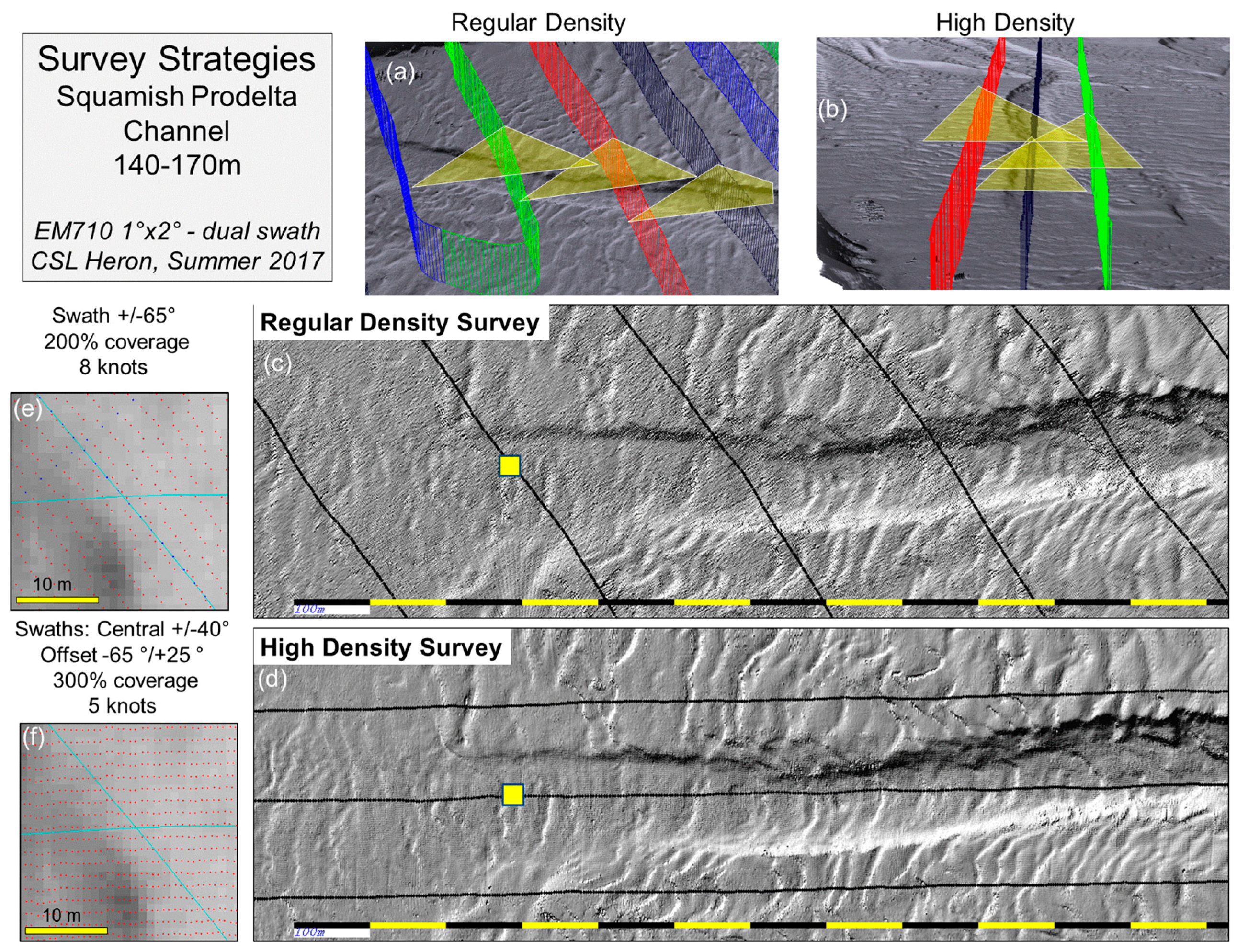
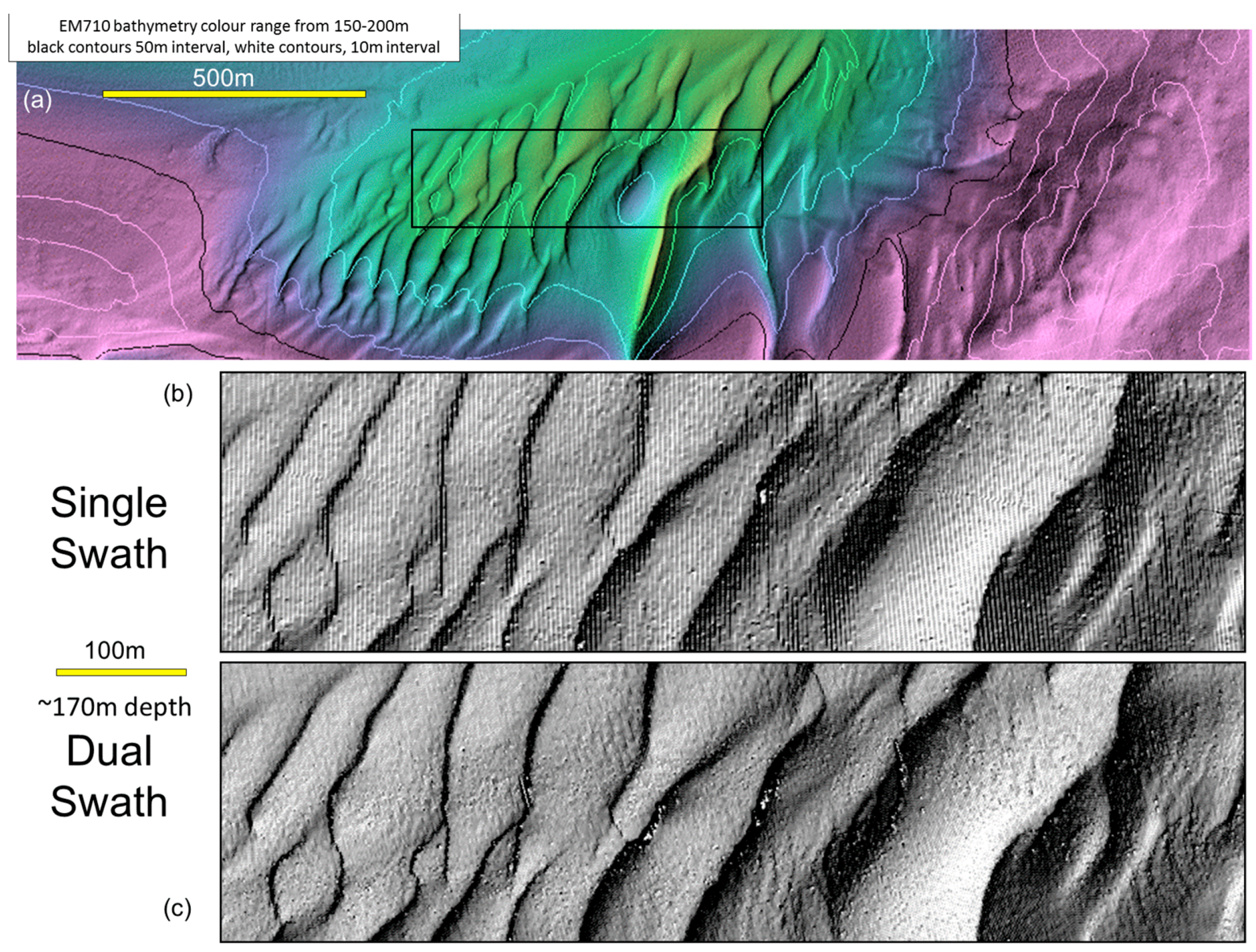
3.3.3. Along-Track Density—Multi-Swath

Even with pitch and yaw stabilization, the along-track density is generally still the limiting factor. A recent innovation is the use of multiple swaths within a single transmission cycle. This is merely an extension of the multi-sector concept, with additional sectors now separated along-track rather than across-track. The net result is the ability to double the along-track data density without compromising swath width.
Figure 10 illustrates the impact of not having dual swath. Two simultaneous passes over the same seafloor have very different definitions of the shorter wavelength population of dunes that sit on the back of the larger dunes. Although both passes have the same across-track beam density, the smaller dunes would be missed without dual swath. Thus, the geomorphometric parameterization could again be compromised.

3.3.4. Sector Width—Within Swath Beam Spacing

Almost all multibeam systems today allow the operator a choice of angular sector over which the finite number of beam forming channels can be redistributed. Thus, at the expense of swath width, the sounding density can be enhanced. Figure 5A shows the significant improvement in the definition of the abyssal dunes when a reduced angular sector is utilized (the data were collected at the same speed). Such a sector width (±25°) is not generally practical, and thus an optimal intermediate setting is usually chosen.
Figure 11 illustrates the impact on resolution over a range of different angular sectors. The target considered is a solitary coral head that lies within a field of sand ripples. Both the coral head and the ripples are typical morphologic features that are of great interest in defining habitat. Yet both are close to the resolution limit of the sonar system. For the reasons discussed in Section 3.3.1, both the along and across-track sounding density increase with reduced swath. Four progressively wider sector widths are utilized. The ripple definition (oriented across-track and thus most sensitive to the along-track density), clearly declines with expanding sector width.
Superimposed on the effects of sounding density, the impact of bottom detection type and signal to noise (discussed in Section 3.2.1) are also visible in Figure 11. The amplitude detection noise (generally within ±15°) is comparable to the vertical scale of the ripple relief and thus gridding coarser, to smooth out the bottom detection noise would also result in removing the real morphology of interest. At grazing angles beyond about 60° where signal to noise issues start to plague the phase detection, the coral head itself becomes poorly resolved. Thus, if boulder definition is of interest, only a subset of a swath corridor can properly characterize their presence and scale (dimensions, spacing etc.).

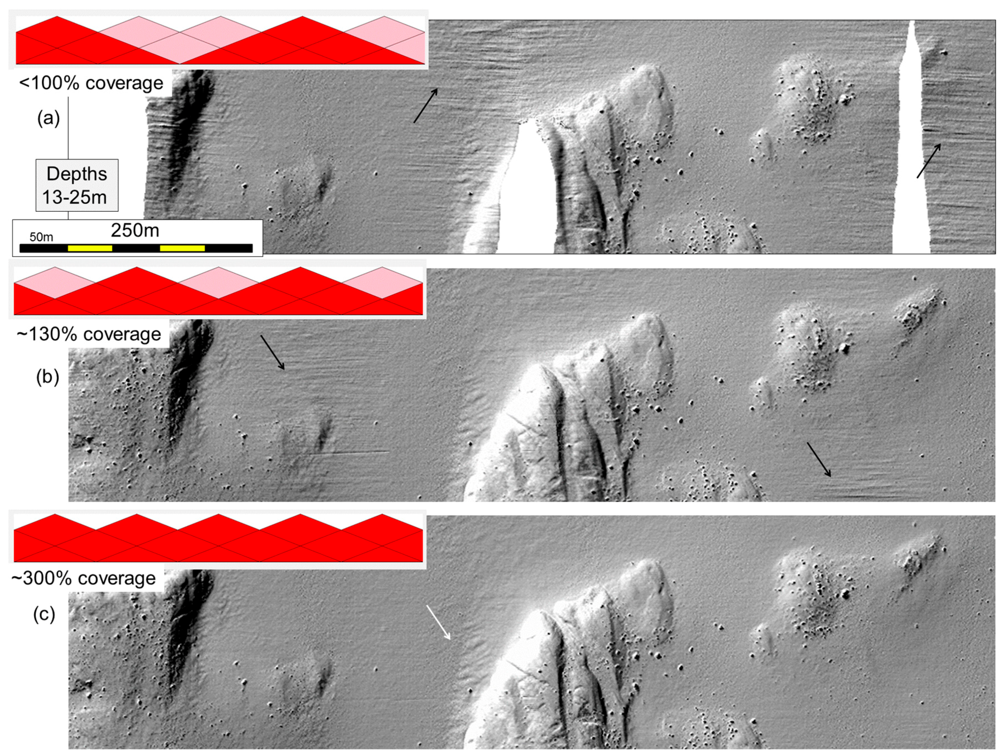
3.4. Corridor Overlap Considerations

For many of the artefacts presented, their manifestation is most apparent in the outer part of the swath corridor (e.g., Figure 5, Figure 6, Figure 8, Figure 9 and Figure 11). Thus, depending on the level of swath to swath overlap, their visibility may or may not be preserved in the final grid product. As long as the gridding process weights the outermost beams lower than the inner beams, higher levels of overlap will progressively remove these features. Figure 12 illustrates progressively higher levels of overlap on the same seafloor.
The data in question, were acquired using a ±72° sector in an area with an undulating near surface thermocline. The net result is a faint residual in the outer swath data (black arrows in Figure 12a). When minimal overlap is utilized (Figure 12b) those features (black arrows in Figure 12b) are maintained in the final grid. If 300% coverage is used (equivalent to utilizing a ±40° sector without overlap), the false relief is absent. Only with this level or overlap does one then adequately resolve the real bedform morphology (white arrow, Figure 12c) that is present whose relief is actually smaller than the artifact.
An alternate approach to increasing overlap seen in Figure 11, could have been to reduce the angular sector so that the noisier outer swath data were not collected at all. This would have the benefit of higher along-track density too. Such an approach works well where there is little topographic variation. In the example here, however, the rock highs are ~50% shallower than the surrounding sedimented areas and thus wider angular sectors allow the minimum coverage requirements to be maintained even if local knolls exist. The geometry utilized in this example was deliberate in order to provide optimal unidirectional low grazing angle backscatter imagery of this terrain.
To best represent a surface, the approaches of Section 3.3.4 and Section 3.4 can be combined by having both narrower sectors and higher overlap density. Figure 13 illustrates the same seafloor alternately surveyed using 200% coverage using a ±65° sector, versus, higher overlap using a ±40° sector and slowing down.
A third party user of a DBM is unlikely to be aware of the underlying source data density utilized. Standard metadata for distributed grids do not usually specify such imaging geometry aspects.

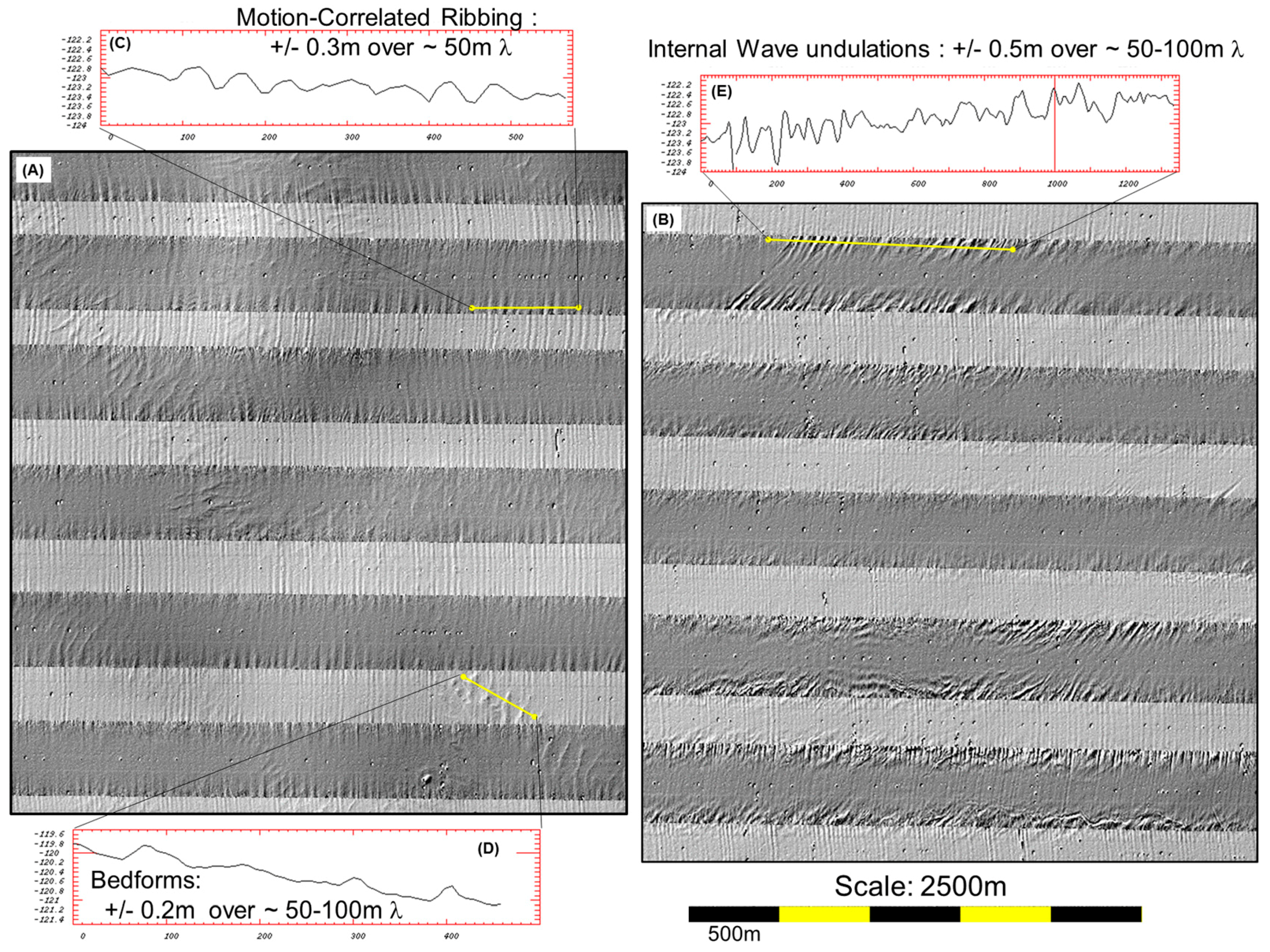
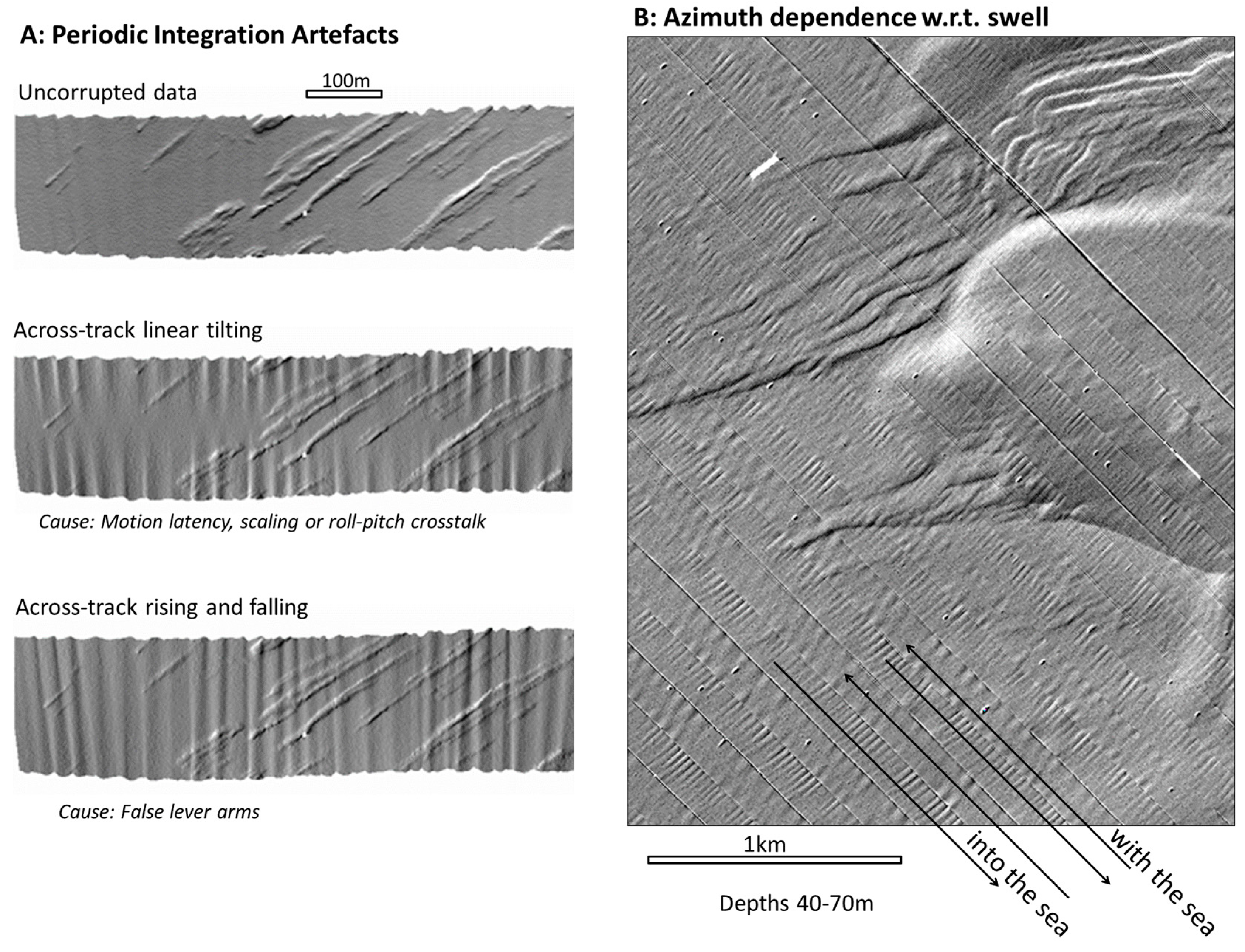
3.5. Motion Residuals

All the previous discussions have assumed that the sonar-relative range and angle solutions are located without compromise due to imperfect position and orientation. With the latest technology, 3D positioning is almost always better than resolution and achievable orientation measurement (<0.02°) is again usually better than beam widths or equivalent angular discrimination through differential phase.
Such benefits, however, are only achieved if the position and orientation is applied correctly as part of the system integration. This requires that the corresponding position/orientation sensor to sonar offset, alignments and timing be at least as good as the source measurements. In reality, this is one of the largest single sources of additional error in multibeam sonar data [24]. The full discussion of the integration imperfections and their impact on the sounding solutions is beyond the scope of this paper, but the reader is referred to [25].
For the purposes of geomorphometric analysis, the main impact is that ship-track orthogonal ribbing in data becomes apparent (Figure 14A). The horizontal spacing of such ribbing reflects the main driving periodic motions of the vessel (the ocean wave spectrum in the 5–15 s period range). With ship speeds of 4–5 m/s this translates to false roughness in the 20 to 75 m range.
Their visibility will vary with seastate and their wavelength will also be significantly affected by the survey line orientation as the apparent wave period is shifted depending on whether the vessel is steaming into or away from the wave direction (Figure 14B). When present, these artifacts are usually immediately apparent to the interpreter as they are clearly orthogonal to the survey direction. They may however, be of a similar amplitude and wavelength to real geomorphic features of interest (as is the case in both Figure 14A,B) and thus would confound automated detection through terrain analysis.

3.6. Sound Speed Residuals

All multibeam beam bottom detection solutions have to be adjusted for the distortion of the initial beam vector by refraction through a layered, heterogeneous ocean. Sound speed profiles are routinely acquired to perform this calculation. A precursor to the beam vector calculation is utilizing the transducer depth sound speed estimate to correctly apply beam steering. If either the beam steering and/or the ray trace calculation is erroneous, false geomorphology may be overprinted on the seabed model.
The simplest artifact is an across-track symmetric, but non-linear distortion (commonly referred to as a smile or frown). This only changes over time constant of 10’s of minutes and will thus only impact swath to swath boundaries (providing false relief parallel to the ship-track at a wavelength of the swath width). While degrading the DBM, this is usually immediately obvious and thus the associated false terrain attribute can be quickly discounted.
What is more concerning for geomorphometric analysis is those sound speed related residuals that result in false short wavelength roughness within a single swath that might be confused with real geomorphology. There are three common types of artifact that come under that description:
  • Heaving towards/away from a strong sound speed gradient.
  • Rolling with an erroneous surface sound speed error.
  • Internal waves or turbulence on a sound speed gradient.
The first two artefacts are clearly motion correlated and are developed strictly ship-track orthogonal and thus appear very similar to the motion artefacts shown in Figure 14. They are distinguished, however, by the fact that the magnitude of the error grown nonlinearly away from nadir. Figure 15A shows a terrain in which across-track ribbing is developed due to motion relative to near surface sound speed fluctuations. Full details of the origin of these can be found in [25].
The third artefact is perhaps the most concerning for analysts looking for short wavelength roughness elements. Applied ray tracing models assume that the sound speed gradients in the ocean occur only in the vertical. If in fact the veloclines are tilted then the ray path will be diverted from that simple assumption. The end result is that if there are wave-like undulations of a sound speed gradient (such as internal waves or turbulence resulting from baroclinic shear), a periodic bathymetric artifact (e.g., Figure 15B) will be projected from the interface onto the seafloor [26].
Figure 15B illustrates the impacts of intense internal wave activity. The data were collected in ~120 m of water in the Celtic Sea during the summertime when a pronounced thermocline is developed and perturbed by tidal activity. A false apparent seafloor roughness is developed preferentially on the edge of the swaths which shows absolutely no correlation from line to line. The artefacts grow nonlinearly toward the edge of the swath. The scale of these artifacts can exceed 1% of depth [26] with wavelengths comparable to or larger than typical shelf bedforms (e.g., Figure 15D). Their orientation is unrelated to the survey line geometry and is often sinuous (see southernmost two lines in Figure 15B), thereby being easy to confuse with real relief. Comparable oceanographically-driven artifacts are common when multibeam data are acquired across abrupt tidal fronts.

4. Discussion

Each of the component limitations of a swath bathymetric system impact the minimum resolvable scale of topographic features. Herein it has been illustrated that the resolution thus varies systematically with depth, with obliquity, with sonar design characteristics and with operator choice of options such as mode, speed and angular sector. The net result is that, within a region of investigation, the achievable resolution will be continuously variable.
Most DBMs utilize fixed grid spacing from which the geomorphometric parameters are derived. Unless the terrain model grid size is chosen to be significantly larger than the poorest achievable resolution, morphologically significant rugosity may appear and disappear within a terrain reflecting the changing imaging geometry rather than the real spatial distribution of natural morphology.
Often, in order to preserve some of the fine scale relief seen in shallower locations, deeper portions of the DBM are gridded finer than is locally justifiable. Under these conditions, uncorrelated sounding noise may appear in those locations and be misinterpreted as natural geomorphic character. That noise is likely to vary systematically across the swath and abruptly with changing sonar settings.
In addition to system resolution limitations, imperfect integration of any of position, orientation or sound speed information can generate false seafloor roughness elements that overprint true geomorphology. Horizontal dimensions for these are typically significantly larger than the sonar resolution and thus can appear similar to natural resolvable features. The vertical scale of these artefacts are usually below the standard hydrography accuracy standards (~±1.3% of depth). Nevertheless, sedimented continental shelves are routinely covered with low relief, long wavelength periodic bedforms whose vertical scale is as little as 0.2 to 0.5% of the depth (e.g., Figure 15D). Thus the presence of these integration artefacts potentially compromises automated geomorphometric analysis.

5. Conclusions

With the growing availability of continuous seafloor terrain models, routine application of geomorphometric classification techniques will become increasingly common. As the interpreter becomes increasingly removed from the field acquisition, however, there is a danger that residual systematic or environmental artefacts in swath bathymetric data may be mistaken for real seabed morphology.
While morphology at scales large with respect to the limit of sonar resolution will usually remain unambiguous, relief close to either the resolution limit or the scale of integration artefacts can be misinterpreted. Unfortunately the resolution limit cannot be easily approximated by a single dimension as this scales with the imaging geometry. Similarly the scale of integration errors is linked to the vessel motion periodicity and scale and the nature of the local oceanography, both of which normally change over the duration of a typical survey period.

Acknowledgments

The author is supported by NOAA grant NA15NOS400002000 and funding from Kongsberg Maritime. Data examples were compiled, with permission, from a variety of sources including the U.S. Naval Oceanographic Office, Kongsberg Maritime (MUNIN AUV, Craig Wallace), the Irish Marine Institute and the Canadian Hydrographic Service.

Conflicts of Interest

The author declares no conflict of interest. The funding sponsors had no role in the design of the study; in the collection, analyses, or interpretation of data; in the writing of the manuscript, and in the decision to publish the results.

References

  1. Fox, C.G.; Hayes, D.E. Quantitative methods for analyzing the roughness of the seafloor. Rev. Geophys. 1985, 23, 1–48. [Google Scholar] [CrossRef]
  2. Shaw, P.R.; Smith, D.K. Statistical methods for describing seafloor topography. Geophys. Res. Lett. 1987, 14, 1061–1064. [Google Scholar] [CrossRef]
  3. Goff, J.A.; Jordan, T.H. Stochastic modeling of seafloor morphology: Inversion of Sea Beam data for second-order statistics. J. Geophys. Res. 1988, 93, 13589–13609. [Google Scholar] [CrossRef]
  4. Mitchell, N.C.; Hughes Clarke, J.E. Classification of seafloor geology using multibeam sonar data from the Scotian Shelf. Mar. Geol. 1994, 121, 143–160. [Google Scholar] [CrossRef]
  5. Lecours, V.; Dolan, M.F.J.; Micallef, A.; Lucieer, V.L. A review of marine geomorphometry, the quantitative study of the seafloor. Hydrol. Earth Syst. Sci. 2016, 20, 3207–3244. [Google Scholar] [CrossRef]
  6. Sánchez-Guillamón, O.; Fernández-Salas, L.M.; Vázquez, J.-T.; Palomino, D.; Medialdea, T.; López-González, N.; Somoza, L.; León, R. Shape and Size Complexity of Deep Seafloor Mounds on the Canary Basin (West to Canary Islands, Eastern Atlantic): A DEM-Based Geomorphometric Analysis of Domes and Volcanoes. Geosciences 2018, 8, 37. [Google Scholar] [CrossRef]
  7. Gardner, J.V. The Morphometry of the Deep-Water Sinuous Mendocino Channel and the Immediate Environs, Northeastern Pacific Ocean. Geosciences 2017, 7, 124. [Google Scholar] [CrossRef]
  8. Diesing, M.; Thorsnes, T. Mapping of Cold-Water Coral Carbonate Mounds Based on Geomorphometric Features: An Object-Based Approach. Geosciences 2018, 8, 34. [Google Scholar] [CrossRef]
  9. Di Stefano, M.; Mayer, L.A. An Automatic Procedure for the Quantitative Characterization of Submarine Bedforms. Geosciences 2018, 8, 28. [Google Scholar] [CrossRef]
  10. Masetti, G.; Mayer, L.A.; Ward, L.G. A Bathymetry- and Reflectivity-Based Approach for Seafloor Segmentation. Geosciences 2018, 8, 14. [Google Scholar] [CrossRef]
  11. Greene, H.G.; Cacchione, D.A.; Hampton, M.A. Characteristics and Dynamics of a Large Sub-Tidal Sand Wave Field—Habitat for Pacific Sand Lance (Ammodytes personatus), Salish Sea, Washington, USA. Geosciences 2017, 7, 107. [Google Scholar] [CrossRef]
  12. Wilson, M.F.J.; O’Connell, B.; Brown, C.; Guinan, J.C.; Grehan, A.J. Multiscale Terrain Analysis of Multibeam Bathymetry Data for Habitat Mapping on the Continental Slope. Mar. Geod. 2007, 30, 3–35. [Google Scholar] [CrossRef]
  13. De Moustier, C. State of the art in swath bathymetry survey systems. Int. Hydrogr. Rev. 1988, 65, 25–54. [Google Scholar]
  14. Lurton, X. An introduction to Underwater Acoustics: Principles and Applications, 2nd ed.; Springer: Berlin, Germany, 2010; Chapter 8. [Google Scholar]
  15. Baltsavias, E.P. Airborne laser scanning: Basic relations and formulas. ISPRS J. Photogramm. Remote Sens. 1999, 54, 199–214. [Google Scholar] [CrossRef]
  16. Ussyshkin, R.V.; Ravi, R. Mitigating the impact of the laser footprint size on airborne lidar data accuracy. In Proceedings of the ASPRS 2009 Annual Conference, Baltimore, MD, USA, 9–13 March 2009. [Google Scholar]
  17. De Moustier, C. Signal processing for swath bathymetry and concurrent seafloor acoustic imaging. In Acoustic Signal Processing for Ocean Exploration; Moura, J.M.F., Louttie, I.M.G., Eds.; Springer: Dordrecht, The Netherlands, 1993; pp. 329–354. [Google Scholar]
  18. Hughes Clarke, J.E.; Gardner, J.V.; Torresan, M.; Mayer, L.A. The limits of spatial resolution achievable using a 30 kHz multibeam sonar: Model predictions and field results. In Proceedings of the OCEANS 98 Conference Proceedings, Nice, France, 28 September–1 October 1998; Volume 3, pp. 1823–1827. [Google Scholar] [CrossRef]
  19. Lurton, X.; Augustin, J.-M. A measurement quality factor for swath bathymetry. IEEE J. Ocean. Eng. 2010, 35, 852–862. [Google Scholar] [CrossRef]
  20. Vincent, P.; Sintes, C.; Maussang, F.; Lurton, X.; Garello, R. Doppler effect on bathymetry using frequency modulated multibeam echo sounders. In Proceedings of the 2011 Oceans, Santander, Spain, 6–9 June 2011; pp. 1–5. [Google Scholar] [CrossRef]
  21. Vincent, P.; Maussang, F.; Lurton, X.; Sintes, C.; Garello, R. Bathymetry degradation causes for frequency modulated multibeam echo sounders. In Proceedings of the 2012 Oceans, Hampton Roads, VA, USA, 14–19 October 2012; pp. 1–5. [Google Scholar] [CrossRef]
  22. Hughes Clarke, J.E. Optimal use of multibeam technology in the study of shelf morphodynamics. In Sediments, Morphology and Sedimentary Processes on Continental Shelves: Advances in Technologies, Research, and Applications; Wiley Online Library: Hoboken, NJ, USA, 2012; pp. 1–28. [Google Scholar] [CrossRef]
  23. Contract Specifications for Hydrographic Surveys, Version 1.2, New Zealand Hydrographic Authority. Available online: https://www.linz.govt.nz/docs/hydro/stds-and-specs/hyspec-v1-2-aug2010.pdf (accessed on 10 February 2018).
  24. Hughes Clarke, J.E.; Mayer, L.A.; Wells, D.E. Shallow-water imaging multibeam sonars: A new tool for investigating seafloor processes in the coastal zone and on the continental shelf. Mar. Geophys. Res. 1996, 18, 607–629. [Google Scholar] [CrossRef]
  25. Hughes Clarke, J.E. Dynamic motion residuals in swath sonar data: Ironing out the creases. Int. Hydrogr. Rev. 2003, 4, 6–23. [Google Scholar]
  26. Hughes Clarke, J.E. Coherent refraction “noise” in multibeam data due to oceanographic turbulence. In Proceedings of the US Hydrographic Conference 2017, Galveston, TX, USA, 20–23 March 2017. [Google Scholar]
Figure 1. Comparing the imaging geometry of an airborne laser scanner and an equivalent resolution inner shelf multibeam sonar. ALS: Airborne (terrestrial) lidar scanner. MBES: Multibeam echo sounder.
Geosciences 08 00109 g001
Figure 2. (left), Effect of changing beam width on the resolution of a specific small target at near normal incidence. EM710 system, 760m depth. (a) 0.5° Tx × 1.0° Rx; (b) 1.0° Tx × 1.0° Rx; (c) 1.0° Tx × 2.0° Rx; (d) 2.0° Tx × 2.0° Rx. (right) illustrating the impact of switching from CW to FM pulse over the same target (again located at near normal incidence). (e) Using a CW pulse; (f) using an FM pulse; (g) resultant apparent topographic relief across a featureless part of the seafloor as observed with the two pulse types (red CW, black, FM).
Geosciences 08 00109 g002
Figure 3. Contrasting the resulting derived digital bathymetric models (DBM) from a surface mounted system in 190 m of water compared with that derived from an AUV flying 20 m off the same seabed. As can be seen the detail on this landslide deposit is markedly clearer. The available scales of derived morphometric parameters are thus quite different.
Geosciences 08 00109 g003
Figure 4. Illustrating the trade-off between AUV coverage and AUV resolution resulting from changing vehicle flying height. EM2040 0.7° × 0.7° system utilizing a ±60° sector. (A) Full swath coverage; (B) zoom of an identically sized (15 × 30 m) area showing the loss in feature definition and relative rise in bottom detection noise with vehicle elevation (the feature alignment is not identical due to limitations in the AUV navigation).
Geosciences 08 00109 g004
Figure 5. Illustrating the identical seafloor as imaged by the same multibeam sonar with different offsets. The seafloor consists of a field of abyssal dunes in 5000 m of water. The dune spacing (~5% of depth) and amplitude (0.2% of depth) is close to the limit of the system resolution (an EM122 1° × 1°). Left: Regional map showing location and orientation of acquired survey lines. (A) Shows an optimal bathymetric rendition acquired with a reduced swath width of ±25° with the ship-track oriented orthogonal to the dune crests; (BF) shows the same area with 5 survey lines using ±65°, each of which is offset 2 km from the next. The same specific dunes are thus observed at 5 different grazing angles while progressing from amplitude to phase detects (and switching to FM pulses at 35°). The white arrowed section indicated the amplitude detection zone.
Geosciences 08 00109 g005
Figure 6. Illustrates the impact on changing from a CW to FM pulse on the identical seafloor. A terrain in ~500 m water depth is imaged by the same sonar sequentially with FM pulses turned on (c,d) and off (a,b). Frames (b,d) show a sun-illuminated representation of the data gridded at ~1% of the water depth. Frames (a,c) show derived sounding noise statistics (one standard deviation scaled by water depth) for the corresponding examples. The location of the sector boundaries is indicated. Ph: phase detection, A: Amplitude detection.
Geosciences 08 00109 g006
Figure 7. Two ±65° swaths of multibeam data collected simultaneously from the same vessel over a seabed in ~35 m water depth. Both sonars have the same transmit and receive beam widths (0.5° × 1.0°). The higher frequency system, however, employs a shorter (higher bandwidth) pulse length (CW: continuous wave). The impact of this is clear in the definition of the short wavelength ripples which are not resolved using the longer pulse.
Geosciences 08 00109 g007
Figure 8. Identical seafloor (~67 m depth) viewed using different available sonar settings. Vessel steaming from left to right. From left to right they are (a) FM pulse—note drop to single swath apparent as across-track ribbing; (b) 0.6 ms CW, with dual-swath so ribbing removed, but note high noise at amplitude (A)-phase (Ph.) transition; (c) 0.2 ms CW, improved and narrower amplitude to phase transition, first resolution of the secondary dune population; (d) 0.07 ms CW, better view of the secondary dunes, but sensitive to noise in outer swath; (e) switching center frequency upward to reduce beamwidth, best view of geomorphology, but with reduced swath width.
Geosciences 08 00109 g008
Figure 9. Impact of multisector yaw and pitch stabilization and dual swath. Two simultaneously acquired swaths of multibeam data (systems mounted on the same vessel): (a) Yaw stabilized coverage (and dual swath); (b) coverage without yaw stabilization; (c) sounding density showing even coverage; (d) sounding density showing irregular coverage.
Geosciences 08 00109 g009
Figure 10. Impact of multi-swath. Two successive passes of the same multibeam system (EM710 0.5° × 1.0°) over a field of multi-scale dunes in 170 m of water. Speeds from 7–9 knots, both passes using a ±65° sector. (a) Regional location; (b) resolved relief using single swath mode; (c) resolved relief using dual swath mode.
Geosciences 08 00109 g010
Figure 11. Impact of sector width choice on achievable resolution. A singular coral head in ~34 m of water, lying within a field of sand ripples, is viewed using the same sonar system (EM710 0.5° × 1.0°) using a range of elevation angles and swath widths. Each subarea view is a 25 m square gridded at 0.25 m resolution which is centered on the known position of the coral head. Each view is at a specific incidence angle (right to left: nadir, 30, 45, 60, 65 and 70 degrees) and with a specific sector width (top to bottom: ±30, 45, 65 and 70 degrees).
Geosciences 08 00109 g011
Figure 12. Impact of swath to swath overlap. Showing the manifestation of oceanographically driven instability in the outer part of a multibeam swath. (a) Full swath extent, including outer beam noise, revealed when <100% coverage is utilized; (b) partial suppression of the outer beam noise when ~30% overlap is used; (c) full suppression over artifact when ~300% overlap is used.
Geosciences 08 00109 g012
Figure 13. Impact of simultaneously changing angular sector, overlap and survey speed. Seabed channel in ~140–170 m of water surveyed twice using the same sensor (EM710 1° × 2°). Regular 200% coverage using ±65° at 8 knots, and ±40° with 300% at 5 knots. (a,b) Illustrate the two survey geometries; (c,d) show the resulting bedform definition (black lines show ship-tracks) and (e,f) reveal the resulting sounding density (zoom of yellow box in (c,d)).
Geosciences 08 00109 g013
Figure 14. (A) The two main characteristics of periodic bathymetric residuals due to imperfect integration; (B) the expression of such residuals over real morphology and the Doppler shifting of the roughness as a function of vessel azimuth w.r.t. swell.
Geosciences 08 00109 g014
Figure 15. (A,B) Showing two different examples of sound speed related artifacts overprinted on a very smooth seafloor in ~120 m of water. The data were collected using a ±61° sector with just 20% overlap. The data are deliberately presented as a sun-illuminated terrain with eastbound lines stenciled separately on top of the west bound coverage. In that manner, the mismatch in the outer swath roughness of the eastbound lines (presented in a darker greyscale) can be compared with corresponding adjacent relief on the westbound lines (a lighter greyscale). Section (C) shows the relief due to motion-correlated errors due to near surface sound speed effects. Section (D) shows the strongest true geomorphic relief (faint sand ridges). Section (E) shows the false topography generated by the passage of an internal wave packet. Further sinuous morphology, indicative of internal wave activity, can be seen on the outer edges of the southernmost two lines.
Geosciences 08 00109 g015

