Modeling Dry-Snow Densification without Abrupt Transition

Abstract

An empirical model for the densification of dry snow has been calibrated using strain-rate data from Pine Island Glacier basin, Antarctica. The model provides for a smooth transition between Stage 1 and Stage 2 densification, and leads to an analytical expression for density as a function of depth. It introduces two new parameters with a simple physical basis: transition density ${\rho }_T$ and a scaling factor, M, which controls the extent of the transition zone. The standard (Herron and Langway) parameterization is used for strain rates away from the transition zone. Calibration, though tentative, produces best parameter values of ${\rho }_T$ = 580 kg m${}^{-3}$ and M = 7 for the region. Using these values, the transition model produces better simulations of snow profiles from Pine Island Glacier basin than the well-established Herron and Langway and Ligtenberg models, both of which postulate abrupt transition. Simulation of density profiles from other sites using M = 7 produces the best values of ${\rho }_T$ = 550 kg m${}^{-3}$ for a high accumulation site and 530 kg m${}^{-3}$ for a low accumulation site, suggesting that transition density may vary with climatic conditions. The variation of bubble close-off depth and depth-integrated porosity with mean annual accumulation predicted by the transition model is similar to that predicted by the Simonsen model tuned for Greenland.

1. Introduction

In the accumulation areas of ice sheets, ice caps, and glaciers, snow is deposited on the surface and, with time, becomes denser until it turns into ice. This process of densification proceeds at a rate that depends on climatic conditions; slowly in the cold, desert regions in the interior of the great polar ice sheets, and more rapidly in warmer regions with higher precipitation. The question of how to calculate this rate from given climatic information is an important aspect of many areas of glaciological research. A recent review [1] cites two problems for which good snow densification models are vital: (1) the determination of past climate from ice-core data and (2) the determination of ice-mass balance changes from altimetry data. In the first case, we wish to know the depth at which snow becomes so dense that bubbles of air are trapped in the ice matrix. This allows an appropriate age to be allocated to chemical constituents of the air. In the second case, we wish to know how changes in climate affect the density profile of snow in order to distinguish between elevation change produced by changes in density and that produced by mass-balance change. Although physics-based snow models, such as CROCUS [2] and SNOWPACK [3,4], were originally developed for hydrological and avalanche forecasting, they have been used successfully to model dry polar snow, but they require detailed initialization and input data that are not always available. There is still a need for simple empirical models that require only the mean annual temperature and accumulation rate as input.

An early suggestion made by Robin [5] has led to a family of empirical-densification models widely used by the glaciological community. He proposed that, in a natural dry-snow cover, the increase in overburden stress is linearly related to the proportional decrease in air volume in the mean density profile. In models based on the Robin hypothesis, strain rate is proportional to a simple function of density. However, from the analysis of density profiles from ice cores, it soon appeared that the proportionality constant changed with density. This problem was overcome by dividing the profile into layers, each with its own constant. Herron and Langway [6] proposed different densification rates for snow with a density of $\rho$ < 550 kg m${}^{-3}$ and 550 kg m${}^{-3}$$\le \rho \le$ 800 kg m${}^{-3}$. Other authors followed suit. This implies a sharp transition between “Stage 1 densification” for lower densities, in which grain-boundary sliding and grain growth are thought to be the dominant mechanisms, and “Stage 2 densification” for higher densities, in which sintering is the primary mechanism. The proposed transition density is the maximum packing density of uniform spheres of ice. However, in natural snow, with a range of grain sizes, high-resolution measurements of density profiles [7] and direct measurements of strain rate [8] suggest that transition density may vary between sites, and that the transition may be gradual.

A better approach to empirical modelling of dry-snow densification might be to accept that strain rate is dependent on a more complex function of density than that proposed by Robin. This would allow a gradual change in densification rate with depth, as the relative importance of grain-boundary sliding, grain growth, and sintering changes. In this paper, a new empirical model of snow densification is proposed, calibrated using field measurements of strain rate as a function of density and validated using high-resolution profiles of ice-core density. The model adds a term to existing models that removes the abrupt transition between Stage 1 and Stage 2.

Snow-densification models need to provide a constitutive law to describe the dependence of volumetric strain rate, $\dot{\epsilon }$, on the applied stress, $\sigma$, and on the strength of the snow, characterised by its bulk density, temperature and sometimes by other variables such as grain size, coordination number [9,10] and impurity concentration [11]. The material-following densification rate is related to $\dot{\epsilon }$ by the definition

$$\dot{\epsilon }=-\frac{1}{\rho }\frac{D\rho }{Dt}$$

(1)

where t is time. In polar firn, there are density fluctuations on an annual or subannual scale about vertically smoothed density ${\rho }_0$ that monotonically increases with depth. In the upper layer of the snow, densification is enhanced by annual and subannual temperature variations, but the amplitude of these variations declines exponentially with depth until, at ≈ 10 m, temperature is close to mean annual temperature $T_m$. The steady-state approximation applies below the surface layer for constant $T_m$ and constant accumulation rate $\overline{a}$.

We begin with the hypothesis that $\dot{\epsilon }$ is a function of ${\rho }_0$ and write

$$\dot{\epsilon }=c\left({\rho }_0\right)\left(\frac{{\rho }_i-{\rho }_0}{{\rho }_0}\right)$$

(2)

where ${\rho }_i$ is the density of ice and $c\left({\rho }_0\right)$ is a site-specific function of density. This implies that the effects of microstructure and impurity concentration on snow strength are secondary compared to the effect of density. The Robin hypothesis states that $c\left({\rho }_0\right)$ is a constant and the dependence of strain rate on density is described solely by the function $({\rho }_i-{\rho }_0)/{\rho }_0$. Hidden within this formulation is an assumption that overburden stress $\sigma$, which increases with water-equivalent depth, is offset by a corresponding increase in snow strength because of some other factor that also increases with depth, such as time since deposition $\tau$.

In the one-dimensional case when horizontal velocity divergence ${\dot{\epsilon }}_H$ is negligible, $\dot{\epsilon }={\dot{\epsilon }}_{zz}$, where

$${\dot{\epsilon }}_{zz}=\frac{\partial w}{\partial z}$$

(3)

We defined a co-ordinate system in which vertical distance z and velocity w are positive upward. Given constant accumulation rate $\overline{a}=-{\rho }_{0}w$, Equations (2) and (3) give

$$\begin{array}{ccc}\hfill c\left({\rho }_0\right)& =& \frac{\overline{a}}{\rho ({\rho }_i-{\rho }_0)}\frac{d{\rho }_0}{dz}\hfill \\ \hfill & =& \frac{\overline{a}}{{\rho }_i}\frac{d}{dz}\left(ln\left(\frac{{\rho }_0}{({\rho }_i-{\rho }_0)}\right)\right)\hfill \\ \hfill & =& -\overline{a}k\left({\rho }_0\right)\hfill \end{array}$$

(4)

In the special case where c is a constant (the Robin hypothesis), its value can be estimated from a single steady-state profile $\rho \left(z\right)$ by plotting the best-fit straight line through logarithmic density function $ln(\rho /({\rho }_i-\rho )$) as a function of z over a section of the profile, say from point z where the water-equivalent height is q to point $z+Z$ where the water-equivalent height is $q+Q$. Writing the (negative) gradient of this line as $-k{\rho }_i$ gives

$$c=-\overline{a}k$$

(5)

where k is a positive constant that we call the vertical densification constant since it is derived from vertical snow density profiles. For simplicity, we call c the density-corrected strain rate whether or not it it is constant.

1.1. Time-Varying Conditions

Given measurements of density ${\rho }_1\left(q\right)$ for a material element at time t and ${\rho }_2\left(q\right)$ for the same element at time $t+\Delta t$, we may calculate the average value of $c\left(\rho \right)$ over time as

$$\begin{array}{ccc}\hfill F(\rho ,q)& =& \frac{1}{\Delta t}{\int }_t^{t+\Delta t}\left(\frac{\rho }{{\rho }_i-\rho }\right)\dot{\epsilon }dt\hfill \\ \hfill & =& -\frac{1}{\Delta t}{\int }_t^{t+\Delta t}\left(\frac{1}{{\rho }_i-\rho }\right)\frac{D\rho }{Dt}dt\hfill \\ \hfill & =& \frac{1}{\Delta t}ln\left(\frac{{\rho }_i-{\rho }_2}{{\rho }_i-{\rho }_1}\right)\hfill \end{array}$$

(6)

In the particular case where c is a constant, the value of F (also constant) can be estimated by averaging over a section of the profile from q to $q+Q$ where Q is several years of accumulation. Then

$$\overline{F}=\frac{1}{Q\Delta t}{\int }_q^{q+Q}ln\left(\frac{{\rho }_i-{\rho }_2}{{\rho }_i-{\rho }_1}\right)dq$$

(7)

Let $-k{\rho }_i$ now be the gradient of the best straight line through a plot of $ln({\rho }_1/({\rho }_i-{\rho }_1)$) as a function of z over the section of the profile from q to $q+Q$ and let $\overline{a}$ be the mean annual accumulation over this section. The indirect method of estimating strain rate from a single density profile is based on the assumption that:

$$\overline{F}\approx -\overline{a}k$$

(8)

by analogy with the steady-state case (Equation (5)). However, if F is not constant over the section of the profile from q to $q+Q$, this indirect method breaks down. This is because at the particular point q, where $F\left(q\right)=\overline{F}$, it is not necessarily the case that the local gradient d ln$({\rho }_1\left(q\right)/({\rho }_i-{\rho }_1\left(q\right)))$/dz = $-k{\rho }_i$.

It is important to remember that, in reality, the accumulation rate is not constant and density profiles can only give an approximate idea of the time-varying, possibly intermittent, densification process that has produced them. Nevertheless, most existing models depend on profile data for calibration since direct measurements of strain rate are so limited. Since the time between storms is a small percentage (say 1%) of the time taken to build up the profile, this should be a reasonable approach.

1.2. Stage 1 and Stage 2 Densification

Herron and Langway [6] suggest an Arrhenius expression,

$$k_0=k_0^{*}exp\left(\frac{-E_0}{\mathrm{R}{T}_m}\right)$$

(9)

for the local (site-specific) Stage 1 vertical densification rate $k_0$. Here, $\mathrm{R}$ = 8.314 J mol${}^{-1}$ K${}^{-1}$ is the gas constant, $E_0$ = (10.16 ± 0.94) kJ mol${}^{-1}$ is the Stage 1 activation energy, $T_m$ the mean annual temperature in degrees Kelvin, and $k_0^{*}$ = 11 (+6, −4) m w.e.${}^{-1}$ is a constant global Stage 1 vertical densification rate. Equation (9) does not necessarily apply to the near-surface layer with a strongly varying temperature. For Stage 2 densification, Herron and Langway propose:

$$k_1={\left(\overline{a}\right)}^{-1/2}{k}_1^{*}exp\left(\frac{-E_1}{\mathrm{R}{T}_m}\right)$$

(10)

where $E_1$ = (21.40 ± 2.26) kJ mol${}^{-1}$ is the Stage 2 activation energy and the constant $k_1^{*}$ = 575 (+152, −121) m w.e.${}^{-1/2}$ a${}^{-1/2}$. Note that, for very low accumulation, this equation can lead to the unrealistic situation of $k_1>k_0$. For example, a model experiment used in the FirnMICE model intercomparison project has $\overline{a}$ = 0.02 m ice a${}^{-1}$ and $T_m$ = −30 ${}^{\circ }$C. In this case, $k_0$ = 0.0722 m w.e.${}^{-1}$ and $k_1$ = 0.1073 m w.e.${}^{-1}$.

If $\overline{F}=F_0$ in the Stage 1 region, and $F_1$ in the Stage 2 region, the Robin hypothesis implies

$$F_{0}exp\left(\frac{E_0}{\mathrm{R}{T}_m}\right)\approx -k_0^{*}\overline{a}$$

(11)

and

$$F_{1}exp\left(\frac{E_1}{\mathrm{R}{T}_m}\right)\approx -k_1^{*}{\left(\overline{a}\right)}^{1/2}$$

(12)

Other authors have suggested modifications to the Herron and Langway model. For example, Arthern and others [12] suggested that both $k_0$ and $k_1$ are independent of $\overline{a}$ from consideration of the physics, and found a good fit to Antarctic strain-rate data from sites with $\overline{a}$ = 0.13–1.04 m w.e. a${}^{-1}$ using

$$k_0=686.7{\mathrm{m}\mathrm{w}.\mathrm{e}.}^{-1}exp\left(\frac{-60{\mathrm{kJ}\mathrm{mol}}^{-1}}{\mathrm{R}T}+\frac{42.4{\mathrm{kJ}\mathrm{mol}}^{-1}}{\mathrm{R}{T}_m}\right)$$

(13)

for Stage 1 and

$$k_1=294.3{\mathrm{m}\mathrm{w}.\mathrm{e}.}^{-1}exp\left(\frac{-60{\mathrm{kJ}\mathrm{mol}}^{-1}}{\mathrm{R}T}+\frac{42.4{\mathrm{kJ}\mathrm{mol}}^{-1}}{\mathrm{R}{T}_m}\right)$$

(14)

for Stage 2. Here, the Naborro–Herring creep (activation energy 60 kJ mol${}^{-1}$) is offset by grain growth (activation energy 42.4 kJ mol${}^{-1}$), so that, for $T\approx T_m$, the effective activation energy is −17.6 kJ mol${}^{-1}$, somewhat higher than the Herron and Langway Stage 1 value and lower than the Stage 2 value.

The Arthern model is attractive because it is firmly-based on physical principles. However, Ligtenberg and others [13,14] found it necessary to add empirical tuning parameters containing $\overline{a}$ to the Arthern model in order to match profiles from Greenland and Antarctica over a wider range of accumulation. They suggest multiplying the r.h.s. of Equation (13) by the ratios

$$MO=1.435-0.151ln\left[\left({10}^3{\mathrm{m}\mathrm{w}.\mathrm{e}.}^{-1}\mathrm{a}\right)\overline{a}\right]$$

(15)

for Antarctic sites and

$$MO=1.042-0.09161ln\left[\left({10}^3{\mathrm{m}\mathrm{w}.\mathrm{e}.}^{-1}\mathrm{a}\right)\overline{a}\right]$$

(16)

for Greenland sites. Similarly the r.h.s. of Equation (14) is multiplied by

$$MO=2.366-0.293ln\left[\left({10}^3{\mathrm{m}\mathrm{w}.\mathrm{e}.}^{-1}\mathrm{a}\right)\overline{a}\right].$$

(17)

for Antarctic sites and

$$MO=1.734-0.2039ln\left[\left({10}^3{\mathrm{m}\mathrm{w}.\mathrm{e}.}^{-1}\mathrm{a}\right)\overline{a}\right].$$

(18)

for Greenland.

Figure 1 shows vertical densification rates $k_0^{*}$ and $k_1^{*}$, implied by these equations, as a function of $\overline{a}$ and $T_m$. In both stages, the Ligtenberg values vary with $\overline{a}$ because of factor $MO$, and with $T_m$ because the activation energy is not the same as the Herron and Langway value. There is a further variation with $\overline{a}$ in Stage 2 because of factor ${\overline{a}}^{-1/2}$, which does not appear in the Arthern and Ligtenberg equations. In both Stage 1 and Stage 2, however, the Ligtenberg values lie mostly within the error bounds of the Herron and Langway values, especially taking into account the fact that, in nature, high accumulation is associated with higher temperatures and vice versa. This is reassuring given that the Herron and Langway model was tuned using a relatively limited set of density profiles. Both models are empirical; the difference is that the Ligtenberg model constrains the activation energy and proposes a more complex dependence on accumulation than the Herron and Langway model.

Simonsen et al. [15] modified the Arthern model by multiplying the r.h.s of Equation (13) by a simple scaling factor $f_0$, and the r.h.s. of Equation (14) by another scaling factor $f_1$ and the terms ${\overline{a}}^{-1/2}$ and exp(−3.8 kJ mol${}^{-1}$/R $T_m$). This produces a Stage 2 expression that follows the Herron and Langway Stage 2 equation in its dependence on $\overline{a}$ and $T_m$. As with the Ligtenberg model, extra parameters are introduced to produce better simulations of field data, but the fundamental assumption of an abrupt transition between Stage 1 and Stage 2 densification is not queried.

In this paper, we tried a different approach. In Section 2, we introduce a new equation for strain rate that allows smooth transition from Stage 1 to Stage 2. We calibrate the parameters of this “transition model” using strain-rate data, making the assumption that the Herron and Langway densification rates for Stage 1 and Stage 2 are correct. We derived the best values of the two new parameters using data from Antarctica and used these values to simulate density–depth profiles from the same area. We then simulated density–depth profiles from other areas and commented on possible changes in parameter values. Finally, in Section 3, we demonstrate the performance of the model using two of the FirnMICE intercomparison experiments.

2. Transition Model

A simple model that removes the abrupt transition between Stage 1 and Stage 2 densification can be constructed using an activation function for c centered around transition density ${\rho }_T$, which is likely to be close to 550 kg m${}^{-3}$ (activation functions are used in artificial neural networks and are not connected with the activation energy in an Arrhenius equation). Let

$$c=\left(\mathrm{D}+\frac{X}{{(1+\mathrm{A}{X}^2)}^{1/2}}\right)$$

(19)

where $X=(\rho -{\rho }_T)$/M${}^{1/2}$ is a scaled density variable describing the distance away from the transition. Away from the transition, A$X^2$ >> 1 and $c\to$ (D −A${}^{-1/2}$) or (D + A${}^{-1/2}$). D and A can be chosen, so that (D − A${}^{-1/2}$)= −$\overline{a}{k}_0$ and (D + A${}^{-1/2}$)= −$\overline{a}{k}_1$, so that c tends toward its Stage 1 and Stage 2 values. Parameter M controls the abruptness of the transition. This particular activation function was chosen because it leads to an analytic solution for the density profile. Other functions that produce a smooth transition from one value to another exist and produce much of the same effect. Note that the assumption is that $k_1$ < $k_0$.

For constant $\overline{a}$, using Equation (4) leads to

$$\int \mathrm{d}z=\frac{\overline{a}}{{\mathrm{M}}^{1/2}}\int \frac{{(1+\mathrm{A}{X}^2)}^{1/2}\mathrm{d}X}{\left(\mathrm{D}{(1+\mathrm{A}{X}^2)}^{1/2}+X\right)\left(\mathrm{C}-X\right)\left(X-\mathrm{B}\right)}$$

(20)

where B = −${\rho }_T$/M${}^{1/2}$ and C = (${\rho }_i-{\rho }_T$)/M${}^{1/2}$. The solution for the integral is given in Appendix A.

Equation (20) allows us to calculate the bubble close-off (BCO) depth, important for the determination of past climate from ice-core chemistry. The transition model also leads to an analytic solution for the depth-integrated porosity (DIP), important for the determination of ice-mass balance from altimetry data.

$$\begin{array}{cc}\hfill DIP=& {\int }_0^z\frac{\left({\rho }_i-\rho \right)}{\rho }\mathrm{d}z\hfill \\ \hfill =& \frac{\overline{a}}{{\rho }_i}{\int }_{X_s}^X\frac{{\left(1+\mathrm{A}{X}^2\right)}^{1/2}\mathrm{d}X}{\left(D{\left(1+\mathrm{A}{X}^2\right)}^{1/2}+X\right)\left(X-B\right)}\hfill \end{array}$$

(21)

where $X_s$ is the surface value of X. The solution for the integral in this equation is given in Appendix B. The BCO depth and DIP are key indicators used in the FirnMICE intercomparison of densification models [1], and are thus useful quantities for demonstrating the effect of using the transition model (Section 3).

2.1. Calibration and Validation

In order to calibrate and validate the new model, detailed measurements of (1) the strain rate as a function of density, or (2) density as a function of depth, are required. There are two sources of such data: repeated nondestructive density profiling in situ using a neutron-scattering technique and high-resolution density profiling of ice cores using gamma-ray attenuation. Over the period from 2004 to 2011, detailed density profiles, at ≈3 cm resolution, were measured in Greenland along the EGIG line [16,17,18] using a neutron probe. From these, strain-rate profiles over periods ranging from a few days to five years could be calculated at the same resolution. Similar repeated density profiles along the iSTAR traverse in the Pine Island Glacier basin, Antarctica, allowed the strain rate of over one year to be calculated [8]. Gravimetric measurements of density are also available from ice cores taken at some of these sites. Höhold et al. [7] provide high-resolution (gamma-ray) core density profiles for a wide range of climatic conditions.

Figure 2 shows the mean annual temperature and annual accumulation rate for each site that could potentially provide calibration or validation data. Note that six iSTAR sites and two core density sites have accumulation rates outside the range used to calibrate the Herron and Langway model, and greater than those found along the EGIG line. We used strain-rate data from the Antarctic sites to calibrate the transition model and define its performance with respect to other models using density profiles from the same sites. We then used density profiles from different sites to (tentatively) validate the model.

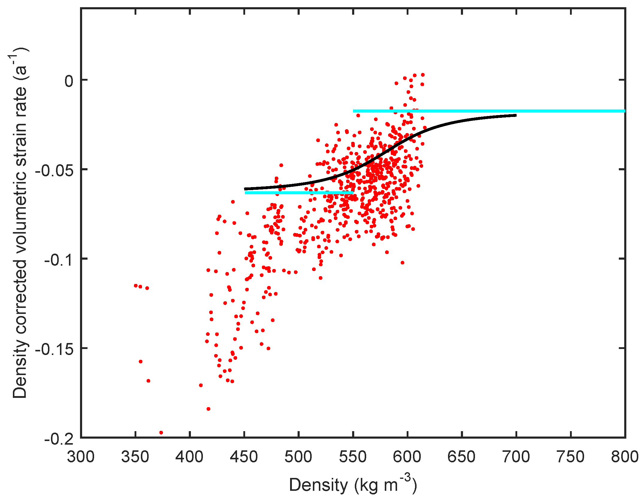
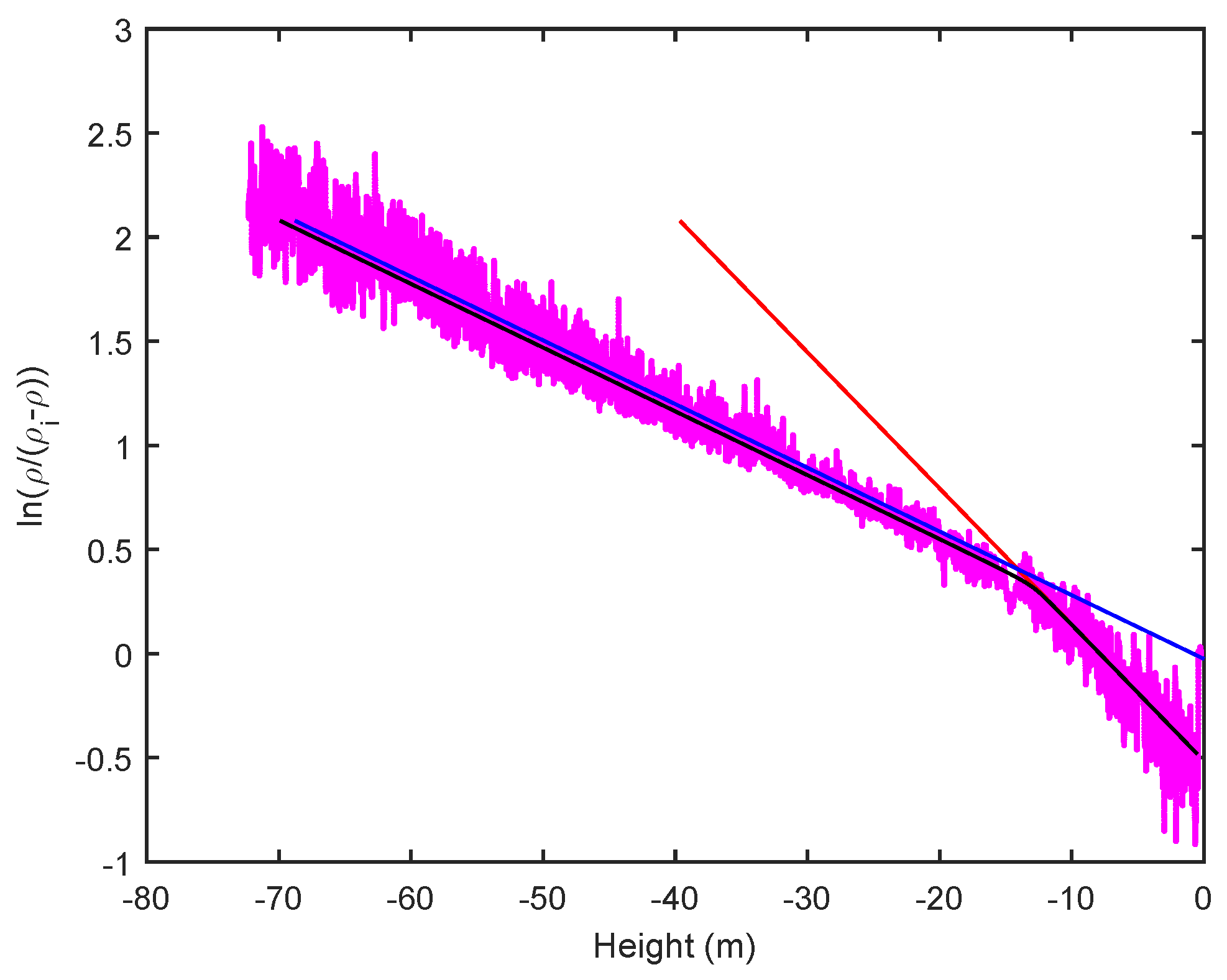
2.2. Strain-Rate Profiles

At most, iSTAR and EGIG line sites neutron probe profiles were obtained at around 13 m depth. At this depth at sites along the EGIG line, density is still below 550 kg m${}^{-3}$, so the data can only be used to determine Stage 1 densification rates, and hence the combination of parameters (D − A${}^{-1/2}$). Even for iSTAR sites, with relatively high surface density, the transition to Stage 2 is not necessarily completed at 13 m depth, so the strain-rate data cannot be used to derive the parameters A and D separately a priori. However, if Stages 1 and 2 densification rates from an existing model are accepted, then at least some of the neutron-probe data can be used to derive suitable values for M and ${\rho }_T$. For simplicity, the Herron and Langway expressions for $k_0$ and $k_1$ are used (Equations (9) and (10)) to calculate A and D.

As an example of the data available from the iSTAR traverse, Figure 3 shows density and volumetric strain rate $\dot{\epsilon }$ as a function of q for iSTAR Site 21 where $\overline{a}$ = 0.75 m w.e. a${}^{-1}$ and $T_m$ = −22.3 ${}^{\circ }$C. The variations in density about the fitted curve show the annual layering. The transition density of ≈550 kg m${}^{-3}$ is reached around 6 m below the surface at $q\approx$ −3.5 m w.e., suggesting that the transition between Stage 1 and Stage 2 densification should be observable at this site. The volumetric strain rate decreases in magnitude with depth, with enhanced values near the surface where summer warming increases the densification rate. The other iSTAR sites showed a similar pattern of behavior.

Figure 4 shows the average density-corrected volumetric strain rate F measured at iSTAR Site 21 as a function of density and the density-corrected volumetric strain rate c predicted by the transition model using best-fit values M = 2.8 and ${\rho }_T$ = 590 kg m${}^{-3}$. The curve for c tends to the values expected from the Herron and Langway model away from the transition density. The values of F are very noisy but it is possible to see that the Herron and Langway densification rates for Stages 1 and 2 are reasonable, provided that a transition region is allowed.

Best-fit values for all sites, taken individually, show wide variation in M, but the values of ${\rho }_T$ cluster around 580 kg m${}^{-3}$. Fixing this parameter and optimizing for M produces 22 values with a mean of 17 ± 8. Excluding three values more than three standard deviations from this mean reduces it to 7 ± 2. Figure 5 shows the effect of using M = 7 and ${\rho }_T$ = 580 kg m${}^{-3}$ at Site 21.

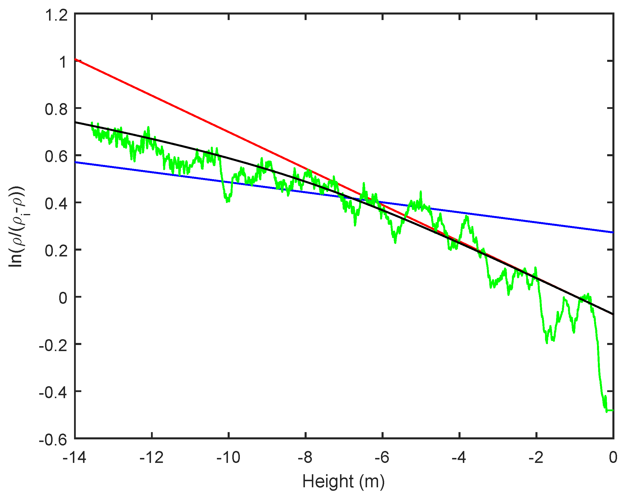
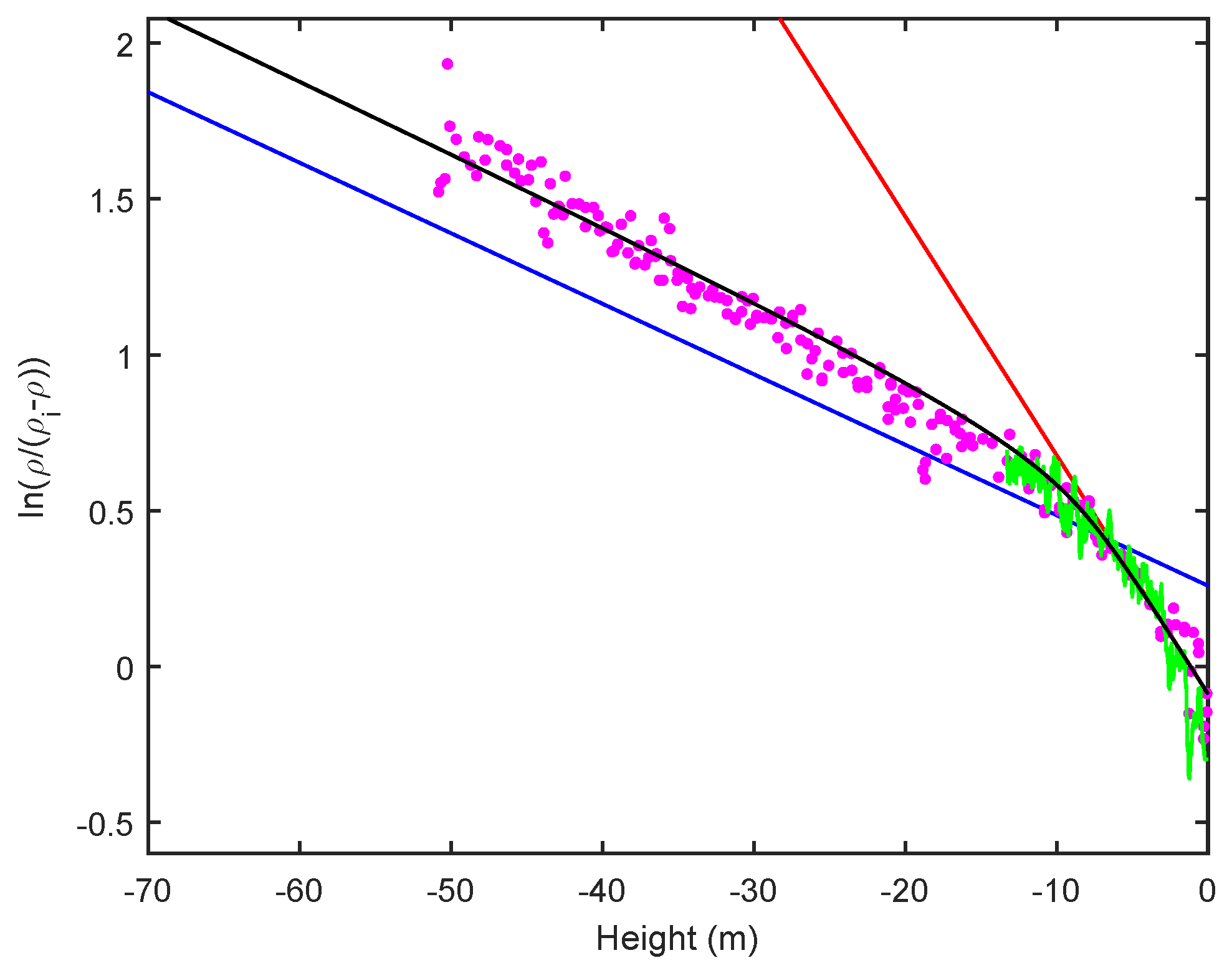
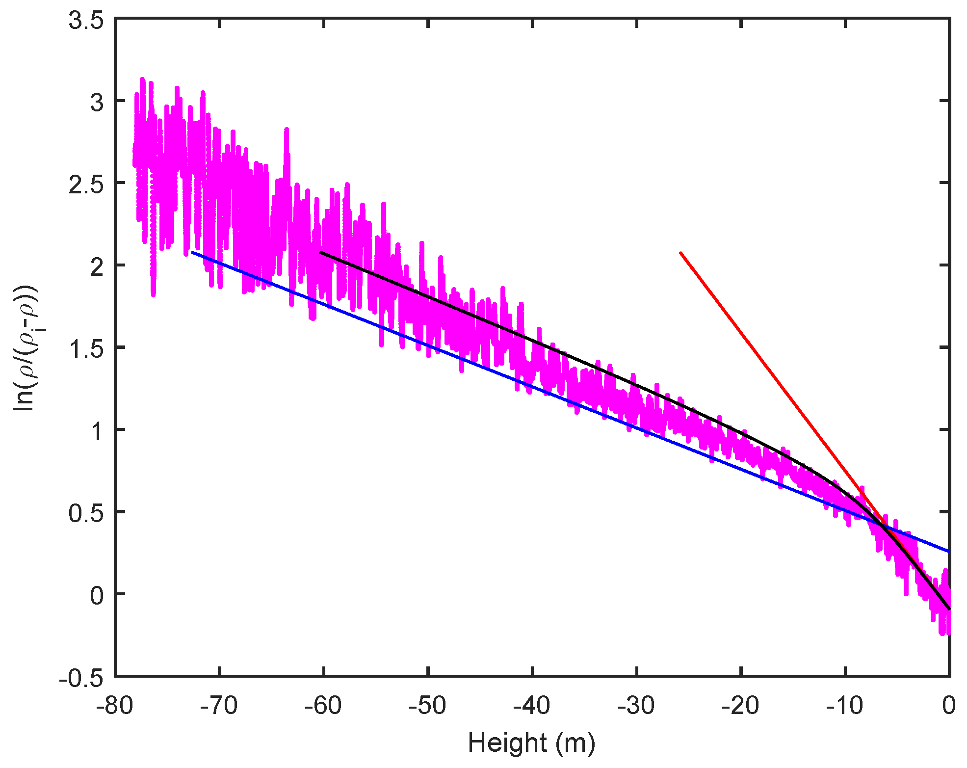
2.3. Density Profiles

Proper calibration of the transition model requires more extensive strain-rate data, ideally from a site with low surface density, so that there is a clear Stage 1 region unaffected by the surface temperature. In order to observe the full transition to Stage 2, data needed to be collected from depths of the order of 20 m. This poses a methodological challenge for neutron-probe measurements. Nevertheless, it was still interesting to investigate the performance of the model as it stands. With the assumption of a constant accumulation rate, this can be done using profiles of ln($\rho /({\rho }_i-\rho ))$ with depth, provided that they are sufficiently detailed.

Figure 6 shows that the transition model does indeed produce a better fit to the neutron probe data at Site 21 than the Herron and Langway model, and that the gradient of a straight line fitted to all the data below the Herron and Langway transition point is greater than the true Stage 2 value to which it tends. Morris et al. [8] defined transitional densification rates, $k_t>k_1$, for densification below $\rho$ = 550 kg m${}^{-3}$, but using the new transitional model makes these unnecessary. As an aside, we note that in the upper 4 m of the profile the densification rate was enhanced by summer warming. Both models would be able to simulate this if snow temperature T rather than the mean annual temperature $T_m$ were used to calculate $k_0$ in Equation (9).

In order to quantify the improvement in fit, we define a cost function

$$\Psi ={\left(\frac{1}{N}\sum {\left(\frac{\left(z_{model}-z_{obs}\right)}{z_{obs}}\right)}^2\right)}^{1/2}$$

(22)

where values of z are calculated at intervals of 5 kg m${}^{-3}$ from $\rho$ = 500 kg m${}^{-3}$. For the neutron probe density profiles, $\rho \left(z\right)$, the sum goes to $\rho$ = 600 kg m${}^{-3}$ and N = 20. The observed values are taken from the polynomial fit ${\rho }_0\left(z\right)$. Thus, the cost function describes the goodness of fit of a given model to the smoothed density data in the deeper part of the profile, where the effect of surface-temperature variations is not significant.

Table 1. Cost functions over the range of 500–600 kg m${}^{-3}$ for the Herron and Langway, Ligtenberg, and transition models for sites in the Pine Island Glacier basin.

Site	$\overline{\mathit{a}}$	Herron and Langway	Ligtenberg	Transition
	m w.e. a${}^{-1}$	$\mathbf{\Psi }$	$\mathbf{\Psi }$	$\mathbf{\Psi }$
1	0.35	0.202	0.185	0.097
2	0.34	0.186	0.148	0.036
3	0.43	0.154	0.098	0.053
4	0.58	0.212	0.162	0.037
5	0.45	0.237	0.217	0.094
6	0.45	0.125	0.076	0.072
7	0.33	0.275	0.250	0.204
8	0.32	0.169	0.133	0.094
9	0.37	0.149	0.125	0.064
10	0.23	0.167	0.083	0.128
11	0.23	0.135	0.060	0.086
12	0.28	0.209	0.155	0.134
13	0.43	0.164	0.129	0.030
14	0.47	0.186	0.162	0.035
15	0.80	0.202	0.284	0.105
16	0.51	0.143	0.110	0.045
17	0.52	0.192	0.140	0.013
18	0.69	0.164	0.163	0.132
19	0.69	0.258	0.219	0.019
20	0.64	0.195	0.156	0.042
21	0.75	0.214	0.181	0.042
22	0.78	0.198	0.170	0.041

shows the cost functions calculated using neutron-probe data from 22 iSTAR sites with mean annual accumulation ranging between 0.23 and 0.80 m w.e. a${}^{-1}$.

At all sites, the addition of the transition model improves the performance of the Herron and Langway model, i.e., reduces the cost function. At all sites except Site 15, which had the highest accumulation, the Ligtenberg model was also an improvement on the Herron and Langway model. However, it is also the case that at all sites except Sites 10 and 11, which had the lowest accumulation, the transition model performed better than the Ligtenberg model.

At some iSTAR sites, ice cores were collected and gravimetric density measurements made to a depth of 50 m. These may be used to extend the neutron-probe data and test the model over a wider range of density. Figure 7 shows a better fit to the neutron probe and core data at Site 4, again obtained by using the transition model rather than the Herron and Langway alone. At this site, $\overline{a}$ = 0.58 m w.e. a${}^{-1}$ and $T_m$ = −23.6 ${}^{\circ }$C.

Table 2. Cost functions over the range 500–800 kg m${}^{-3}$ for the Herron and Langway, Ligtenberg, and transition models for sites in the Pine Island Glacier basin.

Site	$\overline{\mathit{a}}$	Herron and Langway	Ligtenberg	Transition
	m w.e. a${}^{-1}$	$\mathbf{\Psi }$	$\mathbf{\Psi }$	$\mathbf{\Psi }$
1	0.35	0.264	0.145	0.097
4	0.58	0.228	0.092	0.088
6	0.45	0.205	0.106	0.093
7	0.33	0.291	0.287	0.270
8	0.32	0.182	0.114	0.093
10	0.23	0.168	0.116	0.147
15	0.80	0.293	0.186	0.155
18	0.69	0.222	0.137	0.103
20	0.64	0.297	0.184	0.072

shows the cost functions calculated for $\rho$ = 500–800 kg m${}^{-3}$ using a polynomial fit to the core densities to give observed values of z. In this case, N = 60. As before, at all sites, the addition of the transition model improved the performance of the Herron and Langway model, i.e., reduced the cost function. At all sites, including Site 15 this time, the Ligtenberg model was also an improvement on the Herron and Langway model. However, it was again the case that at all sites except Site 10, the transition model performed better than the Ligtenberg model. Although the cost functions in Table 2 place more emphasis on higher densities and less on the transition region than those in Table 1, the conclusions we drew were the same.

Independent high-resolution density data are available from the gamma-ray profiling of ice cores, and provide a test of the transition model in regions outside the Pine Island Glacier basin for which it was optimized. Figure 8 shows data from an ice core (B39) collected in Dronning Maud Land, Antarctica [19], at a site where $\overline{a}$ = 0.77 m w.e. a${}^{-1}$ and $T_m$ = −17.9 ${}^{\circ }$C. The data are available at 1 mm resolution but, in the figure, the data have been smoothed by a 31-point running mean (≈3 cm) for clarity. The model lines terminate at the BCO horizon (the point when density reaches 815 kg m${}^{-3}$ [1]) below which they are not expected to be valid. The cost functions for the Herron and Langway and Ligtenberg models for the density range 500–800 kg m${}^{-3}$ are $\Psi$ = 0.163 and $\Psi$ = 0.156, respectively. Using the transition model with ${\rho }_T$ = 580 kg m${}^{-3}$ and M = 7 produces a cost function of $\Psi$ = 0.128. That is, both the Ligtenberg and the transition model improve on the Herron and Langway fit, with the transition model being better for this high-accumulation site. If ${\rho }_T$ is reduced to 550 kg m${}^{-3}$ an improved fit with $\Psi$ = 0.059 is obtained with the transition model. Note that none of the models predicts the slight increase in densification rate just below the BCO horizon associated with an increase in the density variability. For this, a more complex model including the effect of microstructure and impurities on snow strength would be required [11].

In their analysis of high-resolution (gamma-ray) density profiles, Hörhold et al. [7] noted a weak transition in the slope of the density–depth profiles at densities between 550 and 580 kg m${}^{-3}$ for high accumulation sites (such as B39), whereas lower accumulation sites (such as B26) showed this transition at much lower densities, below 500 kg m${}^{-3}$. Figure 9 shows that a slightly improved fit to the data was obtained with the transition model using ${\rho }_T$ = 530 kg m${}^{-3}$ for core B26 collected in North Greenland [20] at a site with $T_m$ = −30.6 ${}^{\circ }$C and $\overline{a}$ = 0.18 m w.e. a${}^{-1}$. The Herron and Langway cost function $\Psi$ = 0.087 is reduced to $\Psi$ = 0.085. Using ${\rho }_T$ = 580 kg m${}^{-3}$ increased the cost function to $\Psi$ = 0.118. However, even with this transition density, the model performed better that the Ligtenberg model with $\Psi$ = 0.170. It is clear that the transition model could be improved by allowing ${\rho }_T$ to vary with $T_m$ or $\overline{a}$. When more strain-rate data are collected, or more high-resolution (gamma-ray) density profiles are released, this can be investigated.

3. Discussion

The results in the previous section show that the transition model is capable of simulating density profiles through the transition between Stage 1 and Stage 2 more accurately than models with an abrupt transition. This is useful for glaciological problems that require knowledge of transition densities, such as the determination of annual accumulation series from airborne radar data or estimation of past climate from near-surface temperature profiles. More importantly, we note that density profiles are a valuable indirect source of information on strain rates in dry polar snow. By fitting Equation (20) to a density profile we can deduce the parameters of the constitutive law for strain rate, Equation (19). Because of the limitations of the available data, in this paper we have chosen to fix two model parameters (D and A) using the Herron and Langway model, and vary the two remaining parameters (${\rho }_T$ and M). In the future, when more extensive high-resolution measurements of ice-core density are available, one might optimise for all parameters and possibly improve on the Herron and Langway empirical expressions for Stage 1 and Stage 2 densification.

If Stage 2 densification rates are less than Stage 1 rates, the effect of adding a transition zone centered on density ${\rho }_T$ = 580 kg m${}^{-3}$ greater than the usual transition density of 550 kg m${}^{-3}$ will be to increase predicted Stage 2 densities. This would be the case whatever the shape of the activation function and is because densification proceeds at a higher rate over the transition zone before it settles to the Stage 2 value. How important this “over-shoot” is depends on the difference between $k_0$ and $k_1$. If the Herron and Langway values are used, it is clear from Equations (9) and (10) that this difference increases with increasing $\overline{a}$. The consequence is that the transition model predicts BCO depths that are less than those predicted by the Herron and Langway model, by an amount that increases with $\overline{a}$. For the same reason, the depth-integrated porosity (DIP) predicted by the transition model is less than that predicted by the Herron and Langway model. There is some evidence [7] that, at very low accumulation rates, transition density may be less than 550 kg m${}^{-3}$, in which case the BCO depth and DIP would be greater than the Herron and Langway values. This point needs to be explored when more high-resolution field data become available.

Figure 10 shows BCO as a function of accumulation (in this case given in m ice a${}^{-1}$) for $T_m$ = −30 ${}^{\circ }$C, ${\rho }_S$ = 360 kg m${}^{-3}$ and can be compared to Figure 2e in the FirnMICE comparison paper [1]. Using the transition model produces BCO depths that are similar to those predicted by the Simonsen model (using $f_0$ = 0.8 and $f_1$ = 1.25), but greater than those predicted by the Ligtenberg model for Antarctic sites.

Similarly, Figure 11, which can be compared with Figure 2d in the FirnMICE paper, shows that the transition model produces DIP values similar to those of the Simonsen model, and greater than the Ligtenberg values for Antarctic sites.

From Figure 1 we see that, for $\overline{a}$ = 0.1–0.3 m w.e. a${}^{-1}$, the Ligtenberg Stage 2 vertical densification rates are greater than the Herron and Langway rates, so that the difference between the curves in Figure 10 and Figure 11 is as expected. Interestingly, the two tuning parameters added to the Herron and Langway model by Simonsen have much the same effect as the two parameters used in the transition model. However, before taking this comparison too far, we need to remember that the Ligtenberg and Simonsen models were designed for use with different Regional Climate Models (RACMO and HIRHAM5), and the values of $\overline{a}$ and $T_m$ derived from these RCMs are not necessarily the same as the values that would be measured in situ.

4. Conclusions

The transition model provides an alternative way of adapting the Herron and Langway model for density-corrected volumetric strain rates $c_0$ and $c_1$ to produce a better fit to field data, using the same number of extra parameters as the Simonsen model, and fewer parameters than the Ligtenberg model. Of course, it would be possible to combine the transition model with these other models for $c_0$ and $c_1$, although this would produce a less parsimonious model. The attraction of the transition model is that it is based on a simple physical concept that is already well-established in the glaciological literature, that the transition between grain-boundary sliding and sintering as mechanisms for snow densification is a gradual one, and, hence, the two extra parameters, ${\rho }_T$ and M, which describe the location and width of the transition, have a simple physical basis.

References

1. Lundin, J.; Stevens, C.; Arthern, R.J.; Buizert, C.; Orsi, A.J.; Ligtenberg, S.R.M.; Simonsen, S.B.; Cummings, E.; Essery, R.; Leahy, W.; et al. Firn Model Intercomparison Experiment (FirnMICE). J. Glaciol. 2017, 63, 401–422. [Google Scholar] [CrossRef] [Green Version]
2. Vionnet, V.; Brun, E.; Morin, S.; Boone, A.; Faroux, S.; Le Moigne, P.; Martin, E.; Willemet, J. The detailed snowpack scheme Crocus and its implementation in SURFEX v7. 2. Geosci. Model Dev. 2012, 5, 773–791. [Google Scholar] [CrossRef] [Green Version]
3. Wever, N.; Schmid, L.; Heilig, A.; Eisen, O.; Fierz, C.; Lehning, M. Verification of the multi-layer SNOWPACK model with different water transport schemes. Cryosphere 2015, 9, 2271–2293. [Google Scholar] [CrossRef] [Green Version]
4. Steger, C.; Reijmer, C.; Van den Broeke, M.; Wever, N.; Forster, R.; Koenig, L.; Lehning, M.; Lhermitte, S.; Ligtenberg, S.; Miège, C.; et al. Firn Meltwater Retention on the Greenland Ice Sheet: A Model Comparison. Front. Earth Sci. 2017, 5, 1–16. [Google Scholar] [CrossRef]
5. Robin, G.d.Q. Glaciology. III. Seismic shooting and related investigations. In Norwegian-British-Swedish Antarctic Expedition, 1949-52; Norsk Polarinstitutt: Oslo, Norway, 1958; Volume 5. [Google Scholar]
6. Herron, M.M.; Langway, C.C. Firn densification: An empirical model. J. Glaciol. 1980, 25, 373–385. [Google Scholar] [CrossRef]
7. Hörhold, M.W.; Kipfstuhl, S.; Wilhelms, F.; Freitag, J.; Frenzel, A. The densification of layered polar firn. J. Geophys. Res. 2011, 116, 1–15. [Google Scholar] [CrossRef]
8. Morris, E.M.; Mulvaney, R.; Arthern, R.J.; Davies, D.; Gurney, R.J.; Lambert, P.; De Rydt, J.; Smith, A.M.; Tuckwell, R.; Winstrup, M. Snow Densification and Recent Accumulation Along the iSTAR Traverse, Pine Island Glacier, Antarctica. J. Geophys. Res. Earth Surf. 2017, 122, 2284–2301. [Google Scholar] [CrossRef] [Green Version]
9. Arthern, R.J.; Wingham, D.J. The natural fluctuations of firn densification and their effect on the geodetic determination of ice sheet mass balance. Clim. Chang. 1998, 40, 605–624. [Google Scholar] [CrossRef]
10. Brown, R.L. A volumetric constitutive law for snow based on a neck growth model. J. Appl. Phys. 1980, 51, 161–165. [Google Scholar] [CrossRef]
11. Hörhold, M.W.; Laepple, T.; Freitag, J.; Bigler, M.; Fischer, H.; Kipfstuhl, S. On the impact of impurities on the densification of polar firn. Earth Planet. Sci. Lett. 2012, 325–326, 93–99. [Google Scholar] [CrossRef] [Green Version]
12. Arthern, R.J.; Vaughan, D.G.; Rankin, A.M.; Mulvaney, R.; Thomas, E.R. In-situ measurements of Antarctic snow compaction compared with predictions of models. J. Geophys. Res. 2010, 115. [Google Scholar] [CrossRef]
13. Ligtenberg, S.R.M.; Helsen, M.M.; van den Broeke, M.R. An improved semi-empirical model for the densification of Antarctic firn. Cryosphere 2011, 5, 809–819. [Google Scholar] [CrossRef] [Green Version]
14. Kuipers Munneke, P.; Ligtenberg, S.R.; Noël, B.P.Y.; Howat, I.; Box, J.E.; Mosley-Thompson, E.; McConnell, J.R.; Steffen, K.; Harper, J.; Das, S.B.; et al. Elevation change of the Greenland Ice Sheet due to surface mass balance and firn processes, 1960–2014. Cryosphere 2015, 9, 2009–2025. [Google Scholar] [CrossRef] [Green Version]
15. Simonsen, S.B.; Stenseng, L.; Adalgeirsdottir, G.; Fausto, R.S.; Hvidberg, C.S.; Lucas-Picher, P. Assessing a multilayered dynamic firn-compaction model for Greenland with ASIRAS radar measurements. J. Glaciol. 2013, 59, 545–558. [Google Scholar] [CrossRef] [Green Version]
16. Morris, E.; Wingham, D.J. The effect of fluctuations in surface density, accumulation and compaction on elevation change rates along the EGIG line, central Greenland. J. Glaciol. 2011, 57, 416–430. [Google Scholar] [CrossRef]
17. Morris, E.M.; Wingham, D.J. Densification of polar snow: measurements, modelling and implications for altimetry. JGR Earth Surf. 2014, 119, 349–365. [Google Scholar] [CrossRef]
18. Morris, E.M.; Wingham, D.J. Uncertainty in mass balance trends derived from altimetry; a case study along the EGIG line, Central Greenland. J. Glaciol. 2015, 61, 345–356. [Google Scholar] [CrossRef] [Green Version]
19. Wilhelms, F. Density of Firn Core DML96C07_ 39. 2007. Available online: https://doi.pangaea.de/10.1594/PANGAEA.615238 (accessed on 23 October 2018).
20. Miller, H.; Schwager, M. Density of Ice Core ngt37C95.2 from the North Greenland Traverse. 2000. Available online: https://doi.pangaea.de/10.1594/PANGAEA.57798 (accessed on 23 October 2018).
Figure 1. Vertical densification rates for (a) Stage 1 and (b) Stage 2 densification. Black lines show the Herron and Langway values (solid lines) with their uncertainties (dashed lines). Colored lines show the Ligtenberg values for mean annual temperatures of 230 (blue), 240 (cyan), 250 (green), 260 (magenta), and 270 K (red), with solid lines for Antarctic sites and dashed lines for Greenland sites.
Geosciences 08 00464 g001
Figure 2. Mean annual temperature and accumulation at sites for which strain rate data are available (in Greenland [16] and Antarctica [8]), where high-resolution (gamma-ray) core-density profiles are available [7], and where the cores used to calibrate the Herron and Langway densificaton equation were collected [6].
Geosciences 08 00464 g002
Figure 3. Density and volumetric strain-rate profiles from Site 21 along the iSTAR traverse. (a) Density profiles from the austral summers of 2013/14 (red curve) and 2014/15 (green curve), and a fitted polynomial curve showing ρ 0 for 2013/14. (b) Volumetric strain rate at intervals of 1 cm w.e. (red curve) and smoothed over ≈3 cm w.e. (blue curve).
Geosciences 08 00464 g003
Figure 4. Measured values of F as a function of density for iSTAR Site 21 (red dots), values of c for Stage 1 and Stage 2 from the Herron and Langway model (cyan lines) and c as a function of density from the transition model with ρ T = 590 kg m 3 , M = 2.8 (black line).
Geosciences 08 00464 g004
Figure 5. Measured values of F as a function of density for iSTAR Site 21 (red dots), values of c for Stage 1 and Stage 2 from the Herron and Langway model (cyan lines), and c as a function of density from the transition model with ρ T = 580 kg m 3 , M = 7 (black line).
Geosciences 08 00464 g005
Figure 6. Profiles of ln( ρ / ( ρ i ρ ) ) for iSTAR Site 21. Measured values (green), modelled values using Herron and Langway Stage 1 (red) and Stage 2 (blue) densification rates, and modelled values using the transition model with ρ T = 580 kg m 3 , M = 7 (black line).
Geosciences 08 00464 g006
Figure 7. Profiles of ln( ρ / ( ρ i ρ ) ) for iSTAR Site 4. Measured values from ice cores (magenta dots) and neutron-probe profiles (green), modelled values using Herron and Langway Stage 1 (red) and Stage 2 (blue) densification rates and modelled values using the transition model with ρ T = 580 kg m 3 , M = 7 (black line).
Geosciences 08 00464 g007
Figure 8. Profiles of ln( ρ / ( ρ i ρ ) ) for ice core B39. Measured values (magenta line), modelled values using Herron and Langway Stage 1 (red) and Stage 2 (blue) densification rates, and modelled values using the transition model with ρ T = 580 kg m 3 , M = 7 (black line).
Geosciences 08 00464 g008
Figure 9. Profiles of ln( ρ / ( ρ i ρ ) ) for ice core B26. Measured values (magenta line), modelled values using Herron and Langway Stage 1 (red) and Stage 2 (blue) densification rates, and modelled values using the transition model with ρ T = 530 kg m 3 , M = 7 (black line).
Geosciences 08 00464 g009
Figure 10. Variation of steady-state BCO depth with a ¯ using the Herron and Langway (brown line), Ligtenberg (green line), Simonsen (pink line), and transition (blue line) models. Simonsen and Ligtenberg results are taken from [1].
Geosciences 08 00464 g010
Figure 11. Variation of steady-state DIP with a ¯ using the Herron and Langway (brown line), Ligtenberg (green line), Simonsen (pink line) and transition (blue line) models. Simonsen and Ligtenberg results are taken from [1].
Geosciences 08 00464 g011