2.1. Forward Gravity Calculation for a Model with FEM
Using a right Cartesian coordinate system, let
be the rectangular parallelepiped area filled with masses of density
:
Let
denote a position vector of a point in
. Let
be the point of gravity field calculation with position vector
. In this notation the vertical component of gravity field
calculated at
is
where
is the gravitational constant.
A grid-approximation of the parallelepiped density function,
, has the 3D grid
(
,
,
,
,
,
,
,
,
), which constructs elements
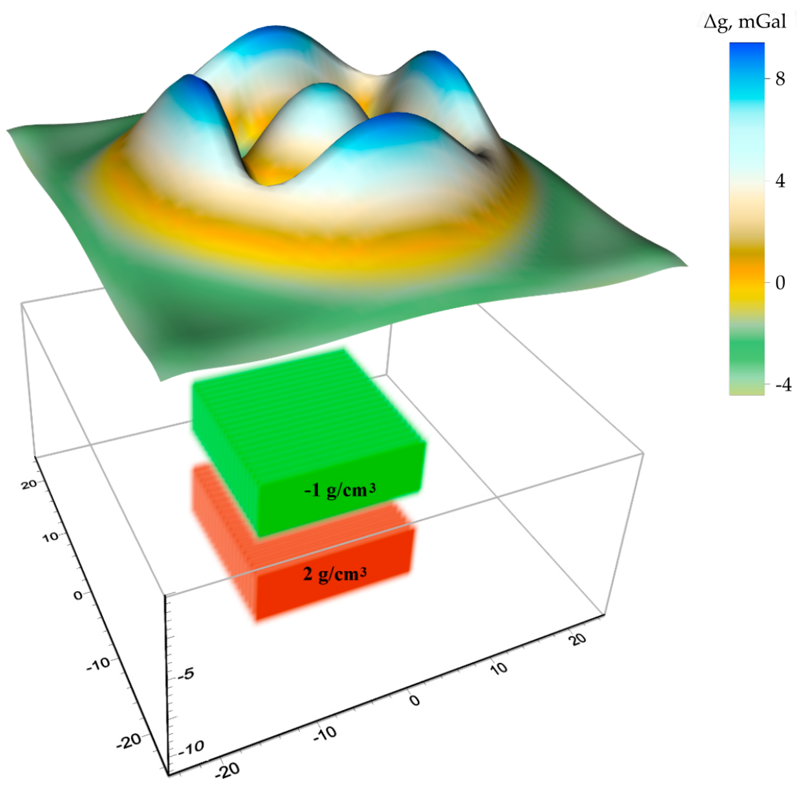
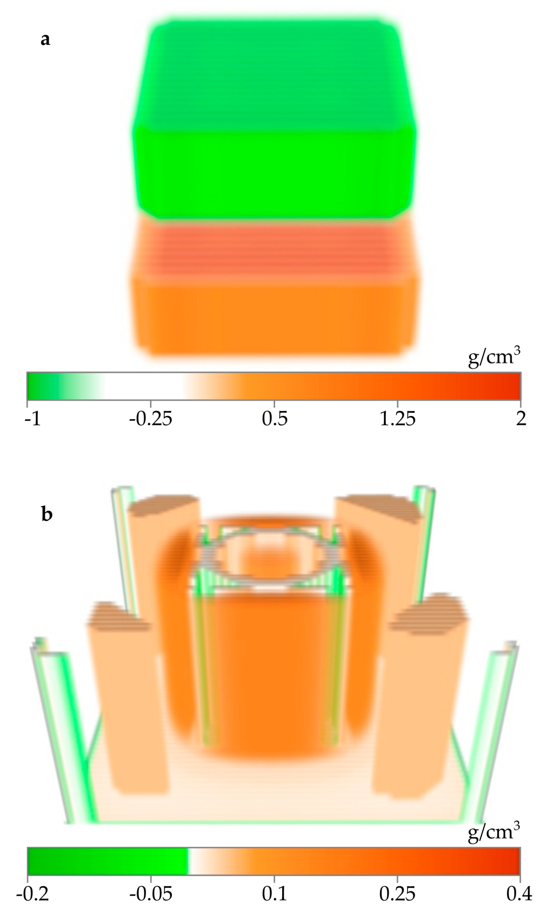
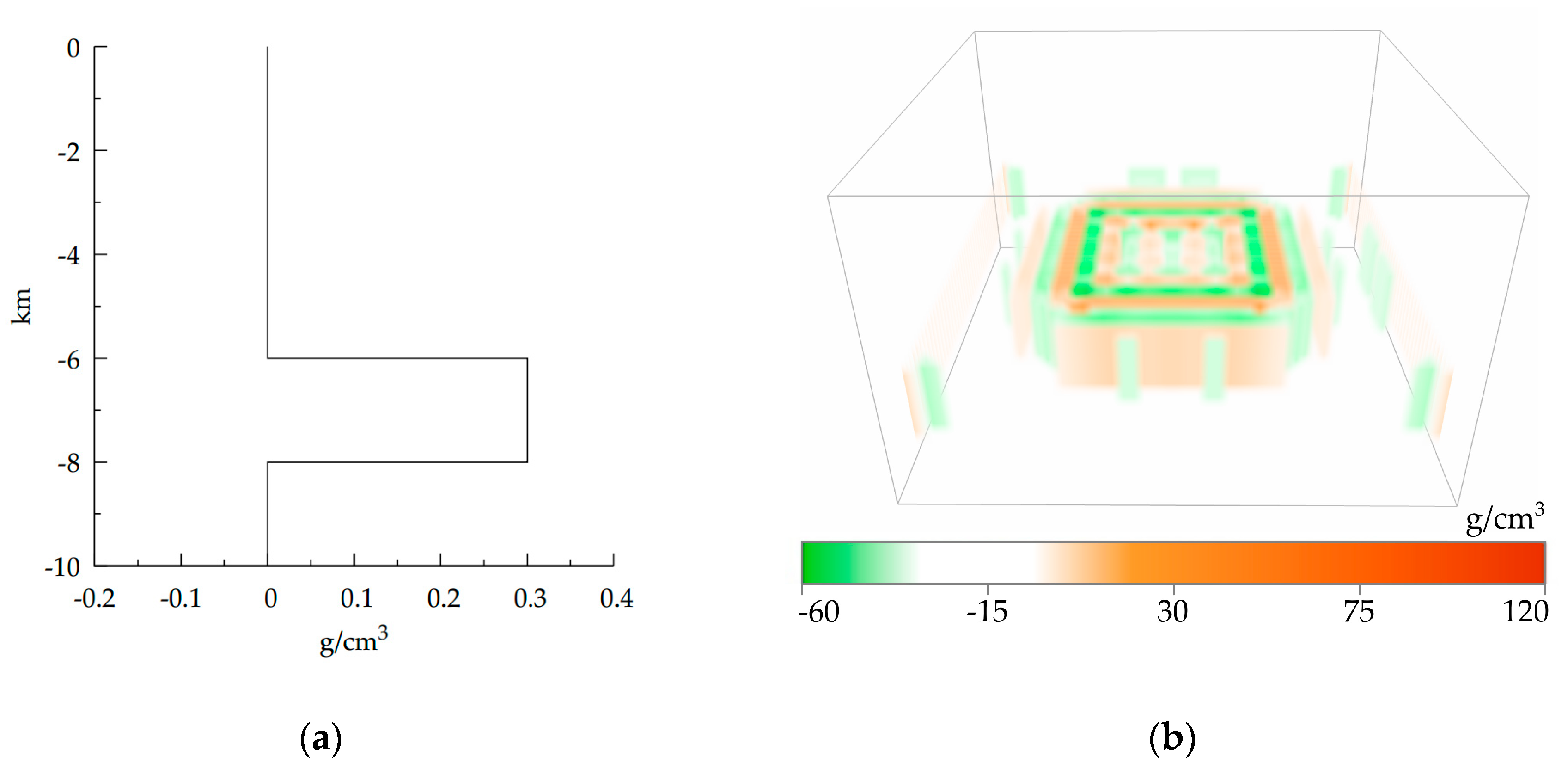
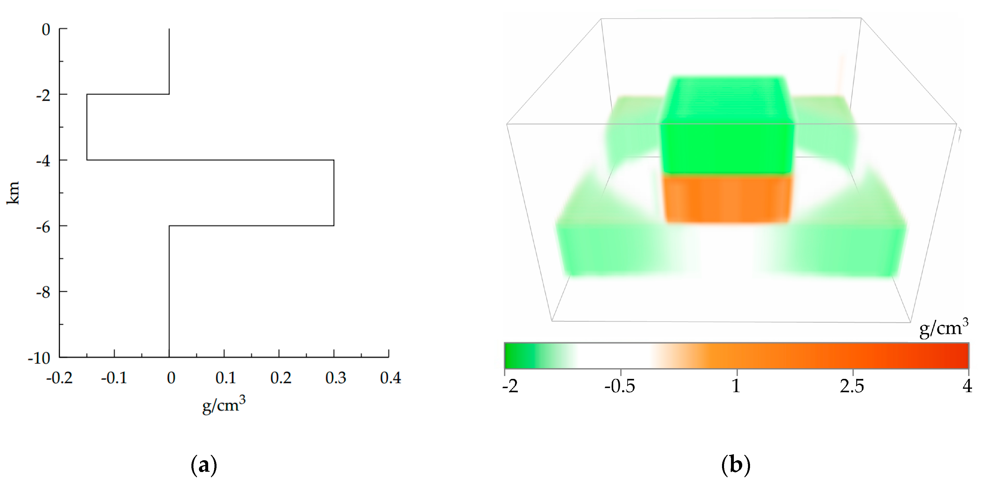
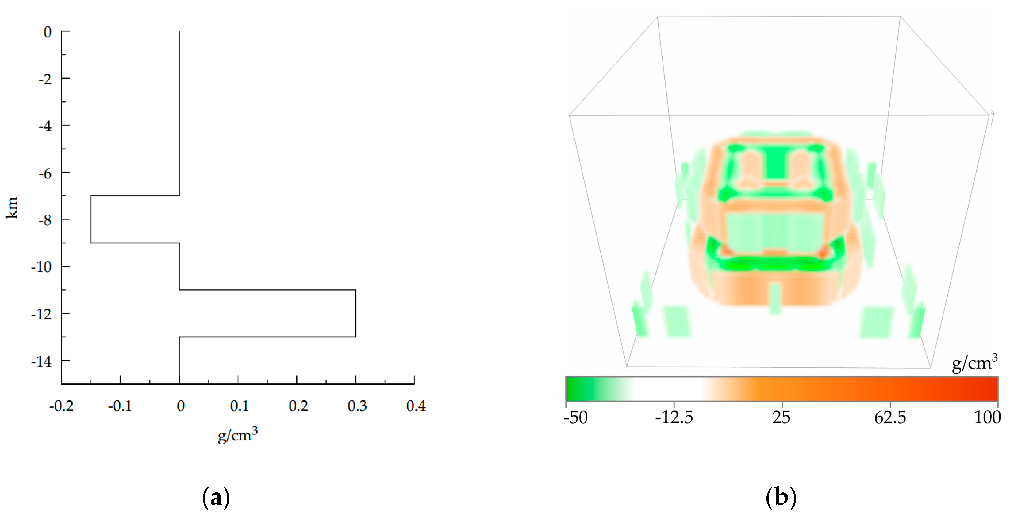
. Element of this three-dimensional grid and its spatial position is presented on
Figure 1.
so the density is a constant for every element:
All parallelepipeds have the same dimensions, so , , , , and , .
Gravity field of a prism with unit density and up to gravitational constant can be calculated with closed form solution formula [
4] as
here
is the gravity effect of the prism
calculated at a point
and
is an expression
. In our case,
, so
;
,
.
And the full gravity field of area
is a sum of fields of prisms
here,
is the density value for the element
Representing the solution in the form of (5) and (6) allows the field calculation algorithm for the layer to be optimized between arbitrary depths.
In practice, it is convenient to calculate gravity field on a flat surface. In this case, all points are located on a single plane. Rectangular grid can be given on this surface. Let this grid be oriented similarly to D and parallel to the D upper face plane. We also assume that the grid step between nodes is and . Thus, a set, , of all field calculation points can be specified as follows: , , , , , , , , .
2.2. Inverse Gravity Problem for Layered Media Model (Density Calculations Using Known Field Values)
The 3D density
calculations in an inhomogeneous area,
D, based on field values,
specified for the point set
, were implemented by inversion of integral operator on the right hand side of the (Equation (2));
g is a known function as measurements. Mathematically speaking, such a problem is ill posed and its solution depends heavily on small variations in the initial field data,
g. However, if we select the density class with only lateral density variations, the determination of the density distribution in the horizontal layer will be stable [
11].
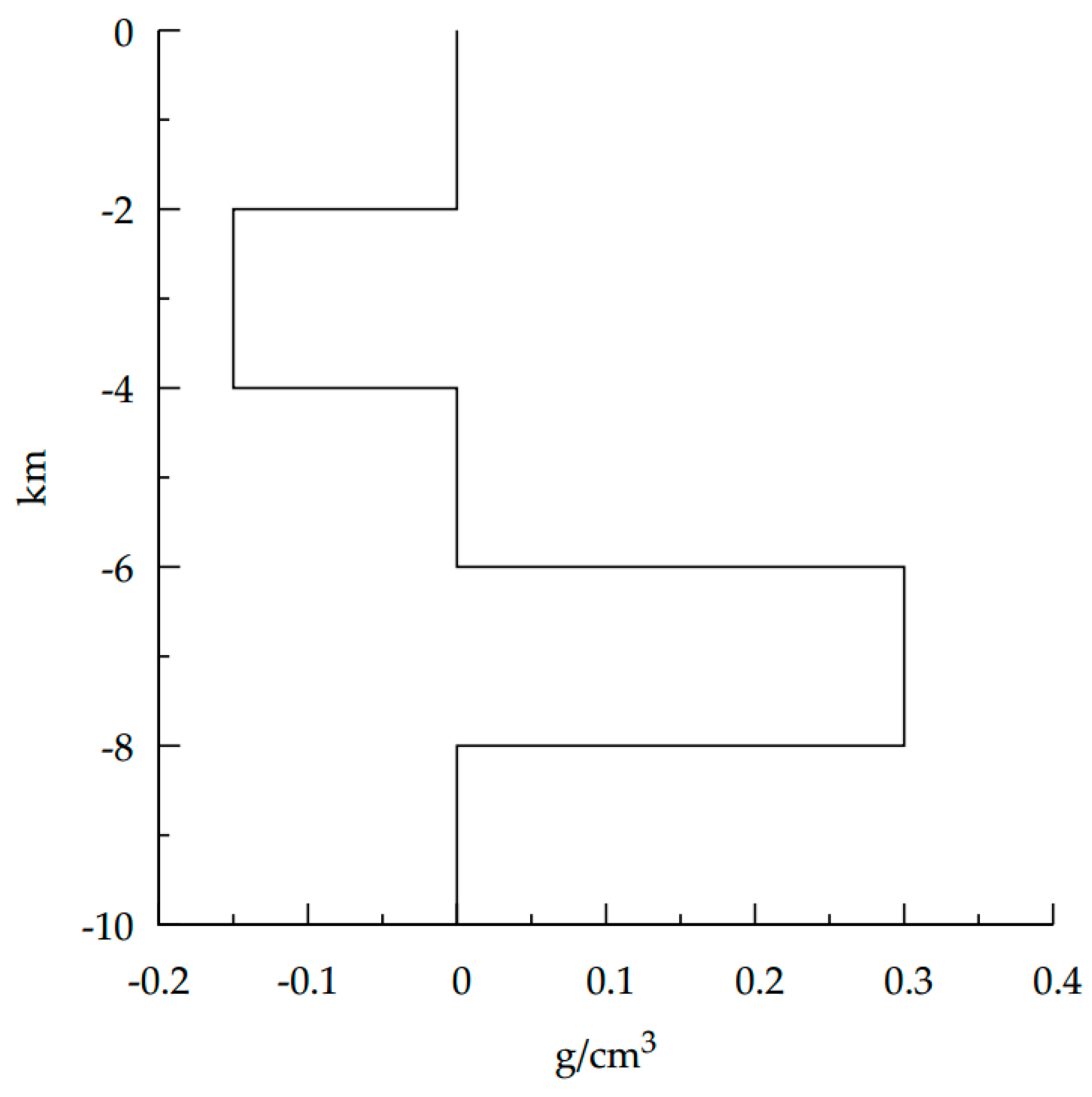
We examined the density for an inhomogeneous parallelepiped with vertical thickness
H as a product that only depends on a depth function,
and
:
We assume
is known from the logging data or may be approximated by some kind of the initial model analysis. Building a grid analogue (4) of the multiplicative density,
, on the partitioning,
, yields
,
;
,
,
,
,
. The field of layered parallelepiped was calculated on a flat surface
. We regroup summands with neighbor indices
and
in sum of (Equation (6)) using the primitive (5):
where
is the difference between the background densities for the
and
horizontal layers:
,
and
,
,
.
To lower the number of the indices in the direct problem operators of (Equation (8)) we introduced the continuous indexing of the density parallelepiped vertical columns:
,
and field calculation points:
,
. If
,
, only one field calculation point (
-th) is located above every density column with index
. We suppose these conditions are further satisfied. For the function
of two variables we have a linear system of equations:
where
is the 3D integration tensor;
is the density increment in depth;
is the unknown lateral density change;
is observed at a height
gravity field value at
-th point.
The value
in (Equation (9)) may be regarded as coefficient for the
. From a physical point of view, it represents the gravity field of a vertical column,
, which is constructed from
elements with densities
:
The problem of determination of density distribution reduces to a linear equation system [
12]
. The
matrix forms from the convolution (10) of the integration tensor with an increment vector and was only calculated once. Any vector of unknowns,
, reduces the 3D parallelepiped field calculations to a trivial matrix vector production operation:
2.3. Inverse Problem Solution Iteration Algorithm
We propose a sustainable adaptive method for solving linear equation systems (11) based on the local corrections method [
13,
14,
15,
16]. However, the original method was created for the reconstruction of boundary surface position. We use it for the density refinement. The method uses the local one-dimensional density distribution model. In our case this means that gravity field income for
-th point
depends only on density distribution in
-th column
. Income from all other columns is ignored for this point.
Consider Equations (8) and (11) for forward gravity calculation as formulas for model field calculation at the points of set
on the level of Earth surface:
. The difference between observed gravity field and the calculated gravity field is the error for inverse problem calculation:
where
is the constant density
the
n-th model column. Then we build an iteration algorithm
calculation. Let
be the difference between fields (12) after
iterations:
This algorithm is based on consequential independent reduction of the remaining
fields at every field calculation point. This reduction was performed by changing
for the vertical density column
. If we assume that the field in point
was produced by the nearest
column mass only and is independent of other columns, then we have only one summand (
) in a sum in (13):
Therefore, the value can be selected as the correction for the -th iteration to a first approximation.
By
variation the field variation at every point is calculated
Adding
to
at every field calculation point we obtain density distribution on
-th iteration:
; model field is calculated as
. Difference (12) between observed and model field on
-th iteration
is the error of the field picking. The stopping condition is the desired accuracy ε achievement:
However, iteration schemes constructed this way generally diverge (
increases) because the ceteris paribus for the contribution of
to the model field at
can be less than the final accumulation of gravity fields of all of the other columns,
. Reducing the square
of the partitioning cell in the
plane increases the divergence because
, and
does not depend on
. Assuming
, we assigned all of the field
values to column
to overestimate the lateral density correction:
. To prevent this overestimate, we assumed
for every iteration.
and
are common to all columns
. The field discrepancy at each point is
where
is the field for the entire parallelepiped
D with
calculated at
.
and
were selected from the minimum condition,
:
In summary, we rewrote the main iteration algorithm stages for selecting values to minimize the discrepancy between the observed and model fields . First, the model field, , and “remaining” field, , are calculated from the initial approximation model. Assuming , cyclically repeat the following steps for iterations:
Calculate by Formula (15).
Calculate and using Formula (18).
Calculate from (17).
Calculate .
Check the stopping conditions: when (i.e., the desired accuracy of ε achieved) or is constant (because the selection has stabilized); if no condition is met, continue with the next iteration, by incrementation .
, ; , , , ,
After executing the density distribution cycle, , ; , , , , , approximates (up to a constant) the difference, , between the observed and initial modeled field. Therefore, adding this distribution to the initial model yields a density model with a field that is closer to the observation with an error of .
2.4. Speed Optimization of Calculations with Forward Problem Formula
Idea of optimization is to replace absolute coordinate values in formulas with relative shifts. To do this we transform Equation (6) into a vector form. The difference
represents a vector between observation and calculation points. It does not contain information about absolute coordinate values anymore. Denote
and reveal in (6)
using Formula (5):
Combining the summands with indices
,
,
and
,
at
yields (by the analogy with the derivation of Equation (8))
assuming
when
.
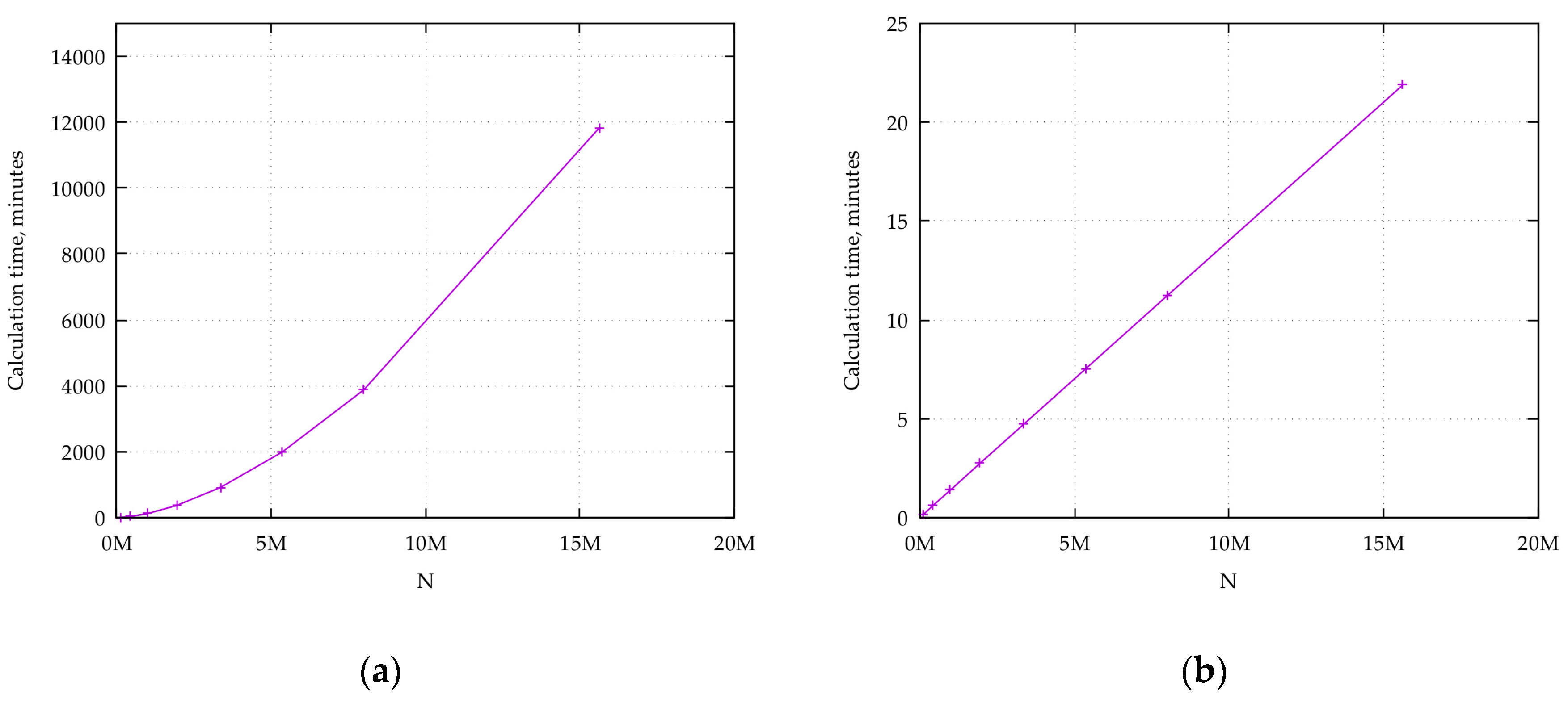
Formula (19) requires to be calculated 8 times, while Formula (20) only requires calculations, which provides an almost eightfold calculation time reduction for a sufficiently large dimension .
For the next optimization, we can write a formula for
set of
values calculated using
set points located in the nodes of the uniform rectangular 2D grid of
size.
Calculating
using Formula (21) requires
be calculated
times. Applying optimization (20) yields:
Using this formula, the
values only need to be calculated
times. However, the specified
in the vector set
exhibits significant overlap and only a single
calculation is needed:
. Introducing new indices
,
,
,
and denoting
allows (22) to be rewritten as
So only needs be calculated for points, which is two orders of magnitude less than using (21) and (22). Notably, there is a possible program implementation for (23) that does not require storing the set in memory. On-the-fly calculations of these elements reduce the memory usage without affecting the performance.
The offered direct problem solution method has two advantages compared to the parallelepiped-based one (Equation (6)): (1) the symmetry of the set with respect to partition D is not required (i.e., the conditions , , , , , are not needed); (2) Equation (23) is two times faster than using Equation (6) even theoretically (and practice indicates larger values yield larger speed advantages) because the “1st step” of Equation (6) calculates the set (described in 1) conditions, which requires calculations of , while (23) under the same conditions requires only calculations.


