Sequential Ensembles Tolerant to Synthetic Aperture Radar (SAR) Soil Moisture Retrieval Errors

Abstract

Due to complicated and undefined systematic errors in satellite observation, data assimilation integrating model states with satellite observations is more complicated than field measurements-based data assimilation at a local scale. In the case of Synthetic Aperture Radar (SAR) soil moisture, the systematic errors arising from uncertainties in roughness conditions are significant and unavoidable, but current satellite bias correction methods do not resolve the problems very well. Thus, apart from the bias correction process of satellite observation, it is important to assess the inherent capability of satellite data assimilation in such sub-optimal but more realistic observational error conditions. To this end, time-evolving sequential ensembles of the Ensemble Kalman Filter (EnKF) is compared with stationary ensemble of the Ensemble Optimal Interpolation (EnOI) scheme that does not evolve the ensembles over time. As the sensitivity analysis demonstrated that the surface roughness is more sensitive to the SAR retrievals than measurement errors, it is a scope of this study to monitor how data assimilation alters the effects of roughness on SAR soil moisture retrievals. In results, two data assimilation schemes all provided intermediate values between SAR overestimation, and model underestimation. However, under the same SAR observational error conditions, the sequential ensembles approached a calibrated model showing the lowest Root Mean Square Error (RMSE), while the stationary ensemble converged towards the SAR observations exhibiting the highest RMSE. As compared to stationary ensembles, sequential ensembles have a better tolerance to SAR retrieval errors. Such inherent nature of EnKF suggests an operational merit as a satellite data assimilation system, due to the limitation of bias correction methods currently available.

1. Introduction

High resolution SAR data has been successfully applied to the estimation of spatially distributed surface soil moisture [1,2]. One of the retrieval methods is to invert soil moisture by matching the backscattering model simulations with the measurements. To simulate the SAR backscattering with the Integral Equation Model (IEM), roughness information is required as a key input [3,4]. The surface roughness in SAR retrievals is usually described as the surface RMS height, correlation length, and Auto-Correlation Function (ACF). These are usually estimated from field measurements of surface height. However, it is widely known that it is difficult to reasonably determine surface roughness in this way [1,5,6]. Contact instruments such as a pin profiler or a mesh board disturb the land surface before measuring the accurate roughness [1]. There are also parallax errors. Non-contact instruments such as lasers, photogrammetry, acoustic backscatter, infrared, or ultrasonic equipment are often interfered with external sources (e.g., wind effects), and sometimes cannot distinguish the effects of topography from optical reflectivity [7]. More importantly, regardless of whether the instruments are contact or non-contact, the roughness measurement in the field is not applicable to spatial estimation, due to a scale dependency [2,5,8]. Thus, as usual, an a priori assumption for roughness is made when simulating a backscattering model [9]. This assumption makes roughness one of main sources of uncertainty. After thorough literature reviews [10,11], it was suggested that SAR retrieval errors are mainly due to roughness (i.e., inversion errors) and that roughness-derived retrieval errors are inevitably present in SAR retrievals, due to spatial heterogeneity, scale discrepancy, roughness measurement errors, inversion errors, and parameterization errors.

Due to such retrieval errors in satellite observations, the bias correction is needed prior to a data assimilation that systematically integrates the model states with the observations [12,13,14,15]. In the field of hydrology, the EnKF method has been widely used to assimilate the microwave-retrieved soil moisture observations into land surface models [16,17,18,19,20,21,22]. For bias corrections, the Cumulative Distribution Functions (CDF) matching has been used [23]. However, it does not always solve the problems, due to complexities of satellite observational errors. There are several issues [12,24,25]. For example, CDF matching aims for a long period of climatology error, although RMSE goals used for validation of satellite data are for instantaneous products. So, it does not consider seasonal dynamics. It also assumes independence from a type of sensors, consequently neglecting retrieval errors specific to instruments and retrieval algorithms used [26]. As it unconditionally converges towards the reference data selected, the analysis is usually vulnerable to the biases of reference data. This limitation is not trivial, as there is no perfect data set to rely on as the reference data. After a bias correction, systematic errors still remain in spatially heterogeneous SAR pixels.

Thus, it is beyond the scope of this study to optimize the roughness conditions at the single local point or to attempt to amend the SAR errors with an imperfect bias correction method that may produce larger errors. Instead, this study aims at assessing how the model states ensembles evolve in the sub-optimal but more realistic conditions for the SAR observational errors. This paper is organized as follows: In Section 2, the site description, land surface models, SAR retrievals, and data assimilation methods are introduced. In Section 3, results and discussions are provided. In Section 3.1 and Section 3.2, the main determinants for SAR retrieval products are specified. In Section 3.3, the point-scale validation of SAR retrievals is provided along with that of the data assimilation analysis. The biases of SAR retrievals are further characterized in Section 3.4 by comparing them with the model. The EnOI and EnKF are compared in Section 3.5 with respect to SAR observational errors defined by Section 3.1, Section 3.2, and Section 3.3. The conclusion and summary are given in Section 4.

2. Methods

Several meteorological instruments for the Global Energy and Water cycle Experiment (GEWEX) Asian Monsoon Experiment on the Tibetan Plateau (GAME-Tibet) were established at the Naqu site [27]. This local station is situated at a latitude of 31.3686 N and a longitude of 91.8987 E. The study domain is defined as the 3 km × 3.5 km area around station BJ on the flat plain [28]. The main land cover within the study domain is sparsely distributed short grassland in bare soil [8,29]. The soil moisture profile was measured at depths of 0.05 and 0.20 m. The rainfall measured on a daily basis was previously shown by Lee et al. [29] and was assumed spatially uniform in this study domain.

This semi-arid region is of a particular interest, as it is difficult to present dry soils with both model and satellite. With respect to satellite retrievals over dry soils, de Jeu et al. [30] previously discussed that the relationship between soil dielectric constant and soil moisture is no longer linear at extremely low moisture contents. That is attributed to an increase in bonds between the soil particle surface and thin films of water surrounding them. With respect to the model, it was previously stated that it is difficult to detect dry soils, because the assumptions used for land surface parametrization or estimation of soil properties are no longer valid at extreme conditions [28,31,32]. Thus, by either models or satellite retrievals, there would be estimation errors over dry soils. For this reason, data assimilation is required for this site to provide the optimal estimates by systematically reducing errors arising from both parties.

2.1. Forecasts: Soil-Vegetation-Atmosphere Transfer (SVAT) Model

The SVAT model simulates a soil moisture profile by water balance. A detailed description of the land surface model scheme was previously provided by [32,33,34]. As shown below, soil moisture is “forced” by atmospheric circulation.

$$\frac{\partial {\theta }_{\text{g}}}{\partial \text{t}}=\frac{{\text{C}}_1}{{\text{d}}_1}\left({\text{P}}_{\text{g}}-{\text{E}}_{\text{s}}\right)-\frac{{\text{C}}_2}{\tau }\left({\theta }_{\text{g}}-{\theta }_{\text{geq}}\right) \text{for} 0<{\mathsf{\theta }}_{\mathrm{g}}<{\mathsf{\theta }}_{\text{sat}}$$

(1)

where, θ_g is surface soil moisture in the top layer d₁, 0.05 m in this study. The first term of right hand side in Equation (1) describes the surface atmospheric exchange activity, while the second term of that indicates water diffusivity. P_g is the precipitation infiltrating into the deep soil layers. E_s is the bare soil surface evaporation rate. τ is a time constant of 1 day. The surface soil variable C₁ and transfer rate variable C₂ in Equation (1) are dimensionless soil coefficients dependent on soil moisture and texture.

$$\frac{\partial {\theta }_{\mathrm{rz}}}{\partial \text{t}}=\frac{1}{{\text{d}}_2}\left({\text{P}}_{\text{g}}-{\text{E}}_{\text{s}}-{\text{E}}_{\text{c}}-\text{Q}\right) \text{for} 0<{\mathsf{\theta }}_{\text{rz}}<{\mathsf{\theta }}_{\text{sat}}$$

(2)

Equation (2) calculates depth-mean root zone soil moisture. P_g adds moisture, while total evapotranspiration (i.e., a combination of E_s and canopy transpiration E_c from the root zone layer d₂ at a depth of 20 cm) and drainage Q withdraw it.

2.2. Observations: SAR Retrievals

2.2.1. Inversion

The Environmental Satellite (ENVISAT) Advanced Synthetic Aperture Radar (ASAR) data operated at C-band (5.331 GHz) and various incidence angles (16°–43°) were used. The VV-polarized swath 1P mode was at a medium resolution of 150 m and a grid spacing of 75 m, resulting in more than 5000 pixels over this study domain. The ASAR data were acquired approximately at 3:50 a.m. (UTC) for descending mode and at 3:50 p.m. (UTC) for ascending mode on Day of Year (DoY) 216 to 224. These days were selected because soils in a dry spell are not altered with other surface conditions changing over time, but we can isolate the effect of roughness only. The short consecutive period was selected for a short-range prediction.

The SAR retrieval was carried out by an inversion approach minimizing mismatches between the backscattering simulations and the measurements. To acquire the ASAR-measured backscattering, the images were calibrated with the Next ESA SAR Toolbox (NEST) software [35]. In parallel with those ASAR measurements, an Advanced Integral Equation Method (AIEM) model also simulated the backscattering coefficients. The AIEM model computes the backscattering coefficients as the sum of the Kirchhoff, the complementary, and the cross term [4,8,36,37].

$${\sigma }_{pp}^o=\frac{{{\displaystyle k}}^2}{2}\text{exp}(-2{{\displaystyle k}}_{\text{z}}^2{{\displaystyle s}}^2){\displaystyle \sum _{\mathrm{n}=1}^{\infty }{{\displaystyle s}}^{2n}{\left|{{\displaystyle I}}_{\text{pp}}^n\right|}^2}\frac{{{\displaystyle \mathrm{W}}}^n(-2{{\displaystyle k}}_{\mathrm{X}},0)}{n!}$$

(3)

where, subscript pp indicates the polarization, k is the wave number, and S is the RMS height. In addition, k_x = ksinθcos$\mathrm{\phi }$, k_y = ksinθsin$\mathrm{\phi }$, k_z = kcosθ, k_sx = ksinθ_scosϕ_s, k_sy = ksinθ_ssinϕ_s, and k_sz = kcosθ_s, where, θ_s and ϕ_s are the zenith and azimuth angles of the sensor, respectively. θ and $\mathrm{\phi }$ are the zenith and azimuth angles of scattering, respectively. I_ppⁿ is a function of the Kirchhoff coefficient and the complementary field of re-radiated fields propagated through two different mediums, and W_n is the Fourier transform of the nth power of the normalized surface correlation function. The AIEM includes the term of surface height at different locations (i.e., a phase factor) in Green’s function and its gradient for multiple-scattering, implying that the upward and downward re-radiations are accounted for [3]. By contrast, a traditional IEM makes the assumptions that the dependency of Kirchhoff coefficients on a slope term is negligible and the local angle can be replaced by some other angles such as incidence angle, ignoring the spatial variability [4].

It simulated backscattering using various incidence angles and soil roughness (a range of RMS height and correlation length) generated in LUTs. For ascending mode, the correlation length ranged from 0.4 to 5.4 (increment: 0.2 cm) and the RMS height ranged from 0.1 to 1 (increment: 0.02 cm), while for descending mode the correlation length ranged from 0 to 5 (increment: 0.2 cm) and the RMS height ranged from 0.22 to 1.12 (increment: 0.02 cm). When the AIEM-backscattering that was simulated at three different incidence angles and roughness conditions described above are matched with the SAR-measured backscattering, those specific roughness conditions were selected. When using the ASAR data acquired at three different incidence angles on adjacent days, the time-invariance of roughness was assumed for those days [1,11,38]. To characterize the surface roughness of the grassland on site, an exponential ACF was selected in the AIEM model [9].

2.2.2. Roughness Experimental Set-up

In addition to the original scheme (control group) described above, other roughness conditions (experimental group) were also manufactured to investigate the error propagation of roughness conditions. Specifically, DoY 221 was selected as it was the driest day of the season based upon field measurements of soil moisture. In a dry condition, the backscattering coefficient is affected mainly by roughness rather than other surface parameters such as the soil dielectric property. Thus, the backscattering coefficient measured on this fixed date was selected to carry out this roughness experiment, instead of time-series data that other conditions change over time (e.g., incidence angle, overpass mode, and soil dielectric constant besides roughness). In other words, it was considered that time-series data interfere with the interpretation of a direct relationship between roughness conditions and soil moisture retrievals.

The roughness ranges in the experimental groups were the derivatives from the optimal roughness in literature. More specifically, as shown in the “s scheme” column of

Table 1. Various a priori roughness conditions.

S Scheme No.	RMS Height (cm)
1	0.05–0.95
2	0.1–1.0
3	0.3–1.2
4	0.4–1.3

, the s scheme used a small increment at 0.02 cm, because of its high sensitivity of the RMS height [39]. The s schemes examine how much roughness errors are systematically propagated when the optimal RMS height is not included in LUTs. For example, s scheme #4 does not include the RMS heights of 0.38, known as the optimal value [8].

2.3. Ensemble Data Assimilation

2.3.1. DEnKF (Sequential Ensemble)

A detailed description of the EnKF theory and algorithm was previously provided [14,17,40]. In this paper, the Deterministic EnKF (DEnKF) is introduced as a sequential ensemble method. In the DEnKF scheme, there is no need to make a random perturbation of observations as in a traditional EnKF in order to prevent the premature reduction in ensemble spread. Instead, it introduces an adaptive inflation. The ensemble evolves forward in time, as follows [41]:

A^a = A^f − 0.5 KHA^f

(4)

where A is the ensemble anomaly (i.e., A_i = X_i − x, where x is the ensemble mean for X_i, the ith ensemble member), superscript a is the analysis, superscript f is the forecast, K is the Kalman gain, and H is the observation operator that relates the model states to the observations. The EnKF provides the final analysis from the mean of the newly updated ensembles. It was previously demonstrated that the DEnKF scheme performed and converged better than a traditional EnKF [41].

2.3.2. EnOI (Stationary Ensemble)

The EnOI scheme has an identical theoretical basis with the EnKF, except that it uses a stationary ensemble of model states [40,42]. Instead of sequentially updating the whole ensemble, the EnOI propagates a single state, as follows [40]:

X^a = X + α PH^T(α HPH^T + R)⁻¹ (d − HX)

(5)

where X^a is the analysis of model state, P is the ensemble covariance matrix, superscript T is the transpose, R is the observation error covariance, d is a vector of the observations, and α is a scaling factor (i.e., α ∈ (0,1]. However, it was not used in this study due to relatively short time integration) for controlling the stationary ensemble. It is considered as a cost-effective way if appropriately optimized [41,43].

2.3.3. Experimental Set-up

Both EnOI and EnKF schemes used the same model ensembles for assimilating the SAR surface soil moisture observations (Section 2.2) into a SVAT land surface model (Section 2.1). The experimental set-up such as the generation of ensemble and observational error was previously provided by [28] and [32]. The ensemble size was 100 [22]. The variance for the observational errors was 0.01, based upon the RMSE of SAR surface soil moisture. Localization, scaling factor, and inflation were not used.

3. Results and Discussions

Through a validation, it was found that the time-average RMSEs of SAR soil moisture is 0.0946 m³/m³. Following sections discuss major determinants responsible for that SAR retrieval error. The potential factors considered include roughness uncertainty, and backscattering measurement errors.

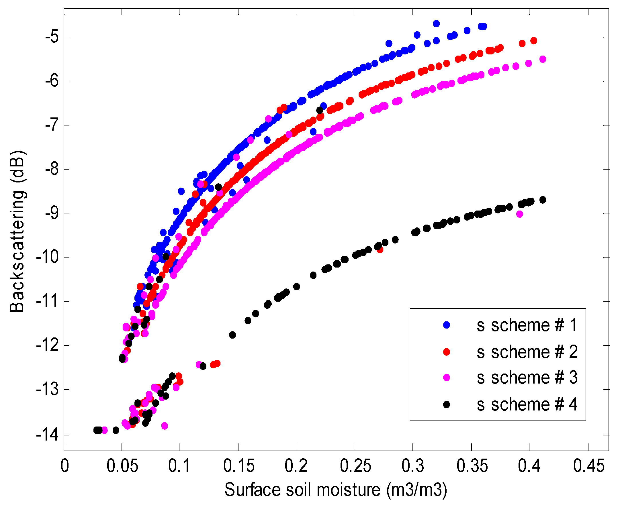
3.1. Propagation of Roughness to SAR Retrievals

3.1.1. Impact of Roughness on the Relationship between Backscattering and Soil Moisture Retrievals: Pixel to Pixel Correspondence

Figure 1 corresponds the ASAR-measured backscattering to the surface soil moisture at the same pixel, which was retrieved differently by the various roughness regimes in Table 1. Except the roughness conditions (i.e., RMS height), all other experimental conditions such as ACF, correlation length, soil dielectric constant, polarization, incidence angle, overpass mode, and frequency were designed to be the same in that figure.

It was shown that the detailed relationships such as slope or dispersion of data points vary by roughness conditions [10,39]. Despite the small increment, the s scheme in sub-optimal conditions non-linearly propagated soil moisture retrievals, ultimately making the large spreadsSpecifically, s scheme #4 in Figure 1 largely deviated from other s scheme groups including optimal value in LUTs, although its increment is the same at 0.02 cm. This is considered because the s scheme #4 ranging from 0.4 to 5.4 cm does not include the optimal RMS height of 0.38 cm [8]. This finding of the non-linear amplification of the roughness errors under sub-optimal roughness conditions is consistent with previous studies [5,9].

Table 2. The different spatial averages of soil moisture products by roughness schemes.

S Scheme No.	1	2	3	4
Roughness (cm)
-	0.218	0.246	0.365	0.438
Resultant soil moisture retrievals (m3/m3)
-	0.1449	0.1356	0.1080	0.1054

also shows that a spatial average of soil moisture retrievals was largely altered by the s scheme. From Figure 1 and Table 2, it was found that the RMS height has an inverse relationship with soil moisture [44], implying that surface becomes smoother if soil porous media is filled with water. In other words, higher RMS heights (s scheme #4) estimated drier. It is considered that such an inverse relationship between surface roughness and soil moisture is attributed to a negative exponential function of roughness as shown in Equation (3). Similarly to this result, previous studies [45,46] also carried out the similar sensitivity analysis of the radar signal to various land surface parameters over short grass, and found that the most influencing parameter is the surface roughness. However, this impact may be different in different incidence angle or land cover conditions.

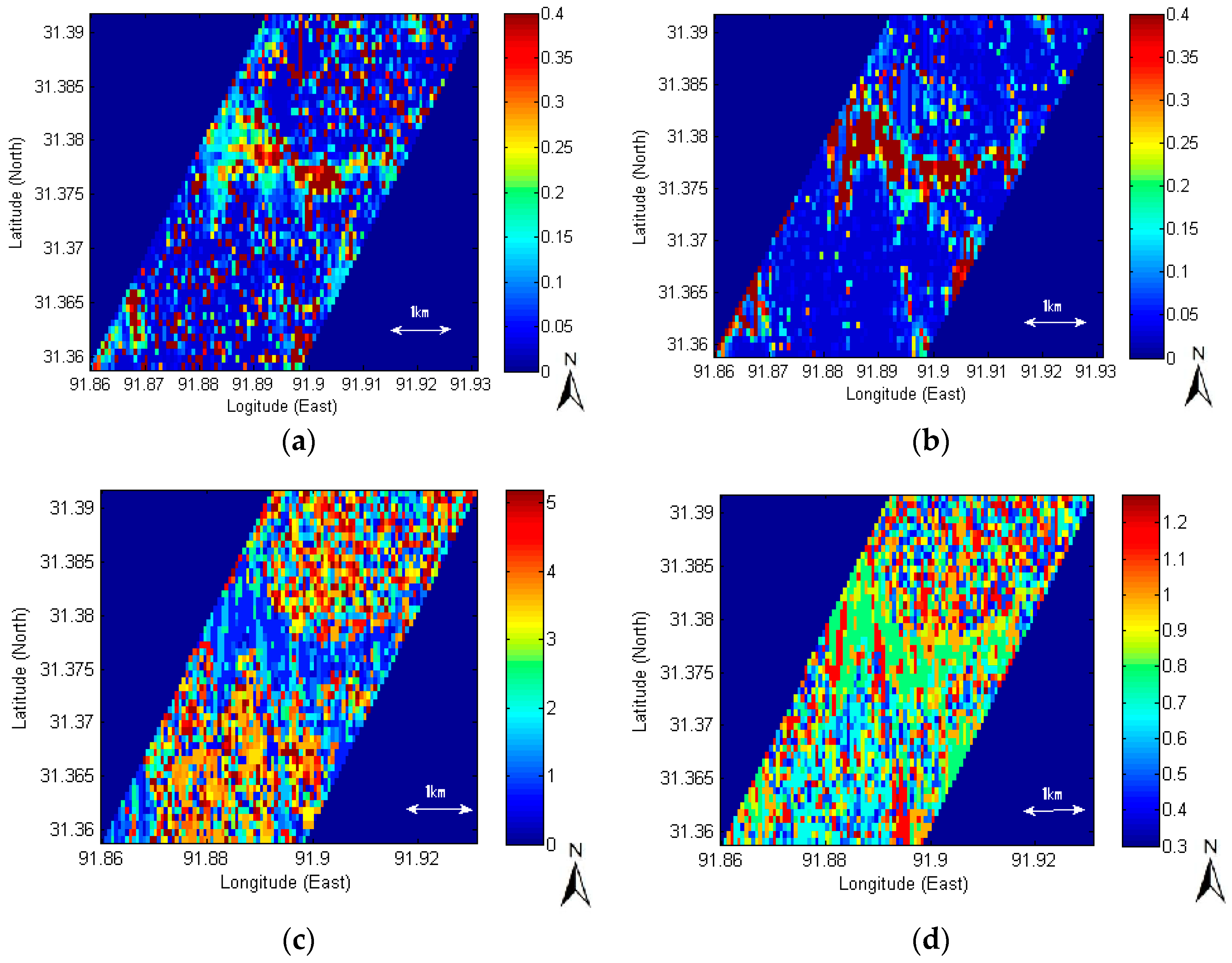
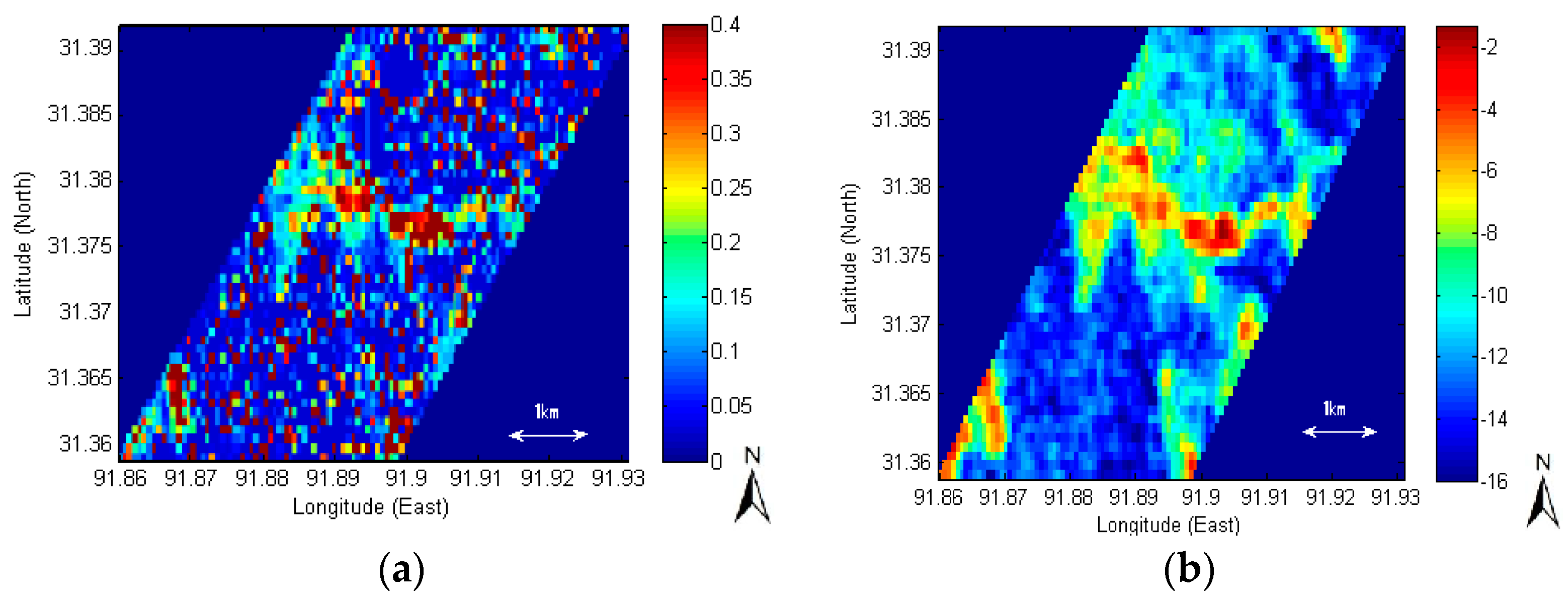
3.1.2. Impact of Roughness Errors on Soil Moisture Retrievals: Spatial Distribution

The surface soil moisture was differently retrieved by various roughness schemes. In particular, each roughness scheme produced a different spatial distribution. To effectively illustrate the systematic propagation of roughness conditions, two schemes that have contrast with each other were selected and demonstrated in Figure 2. For example, the s scheme #2 (Figure 2a) reported several overestimations in the dry area, while the parts overestimated by s scheme #4 (Figure 2b) were limited to the wet area only. Here, the “wet area” is defined as the area at latitude of 31.375 to 31.385, while “dry area” is a remaining part except the wet area. Considering that there had been no rainfall events for several days until DoY 221, that the field measurements also showed the driest condition on this day, and that the only difference between Figure 2a,b is roughness (in specific, correlation length is shown in Figure 2c, and RMS height in Figure 2d, respectively), it is evident that Figure 2a was over-estimated, due to roughness inversion errors. From that, it was suggested that lower RMS height (s scheme #2) estimated the wet area better than higher RMS heights (s scheme #4). In other words, the soil moisture retrievals were considerably overestimated by s scheme # 2 (Figure 2a), showing several overestimations over the dry area as indicated by red points. On the other hand, the same dry area was appropriately estimated dry by s scheme #4 (Figure 2b). There was a high sensitivity of roughness to final soil moisture retrievals.

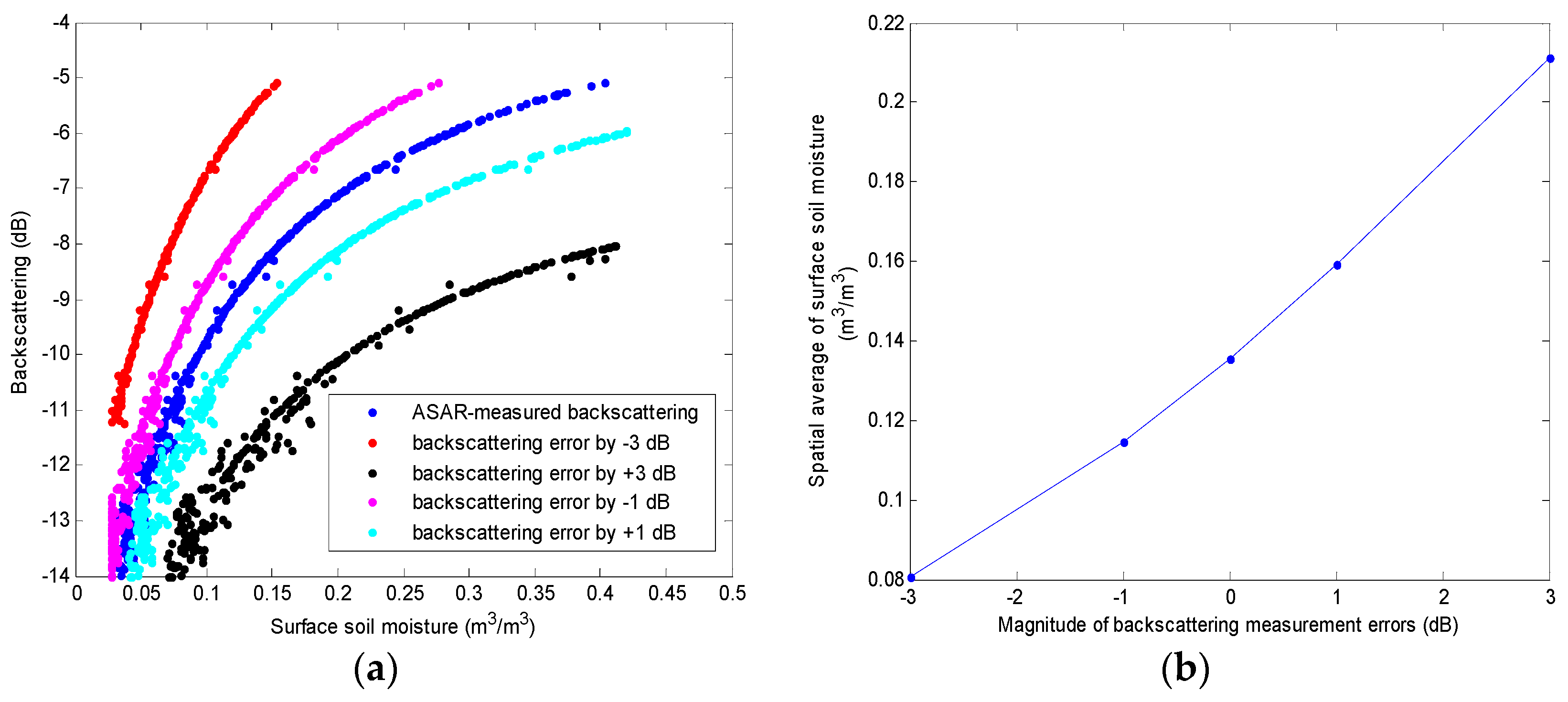
3.2. Propagation of ASAR Backscattering Errors on SAR Retrievals

To more systematically assess the magnitude of roughness inversion error propagations, the results in Section 3.1 were further compared with other sources of retrieval errors: backscattering measurement error (e.g., calibration errors, vegetation attenuation). Especially in arid or semi-arid regions covered with short grassland, as in the Naqu site of this study domain, the multiple backscattering effects from vegetation added to or subtracted from moisture in the underlying soil generate measurement errors. Studies [47,48,49] previously suggested a simple correction model for vegetation effects. However, in practice, it is difficult to widely apply that to diverse regions, because canopy and instrumental characteristics should be thoroughly specified.

3.2.1. Impact of Backscattering Errors on the Relationship between Backscattering and Soil Moisture Retrievals: Pixel to Pixel Correspondence

To investigate the error propagation of backscattering, it was hypothesized that backscattering measurement errors range from ±1 dB to ±3 dB, based upon [1,10] that suggested the similar measurement error ranges arising from vegetation effects or calibration errors of ENVISAT ASAR and ERS-1 SAR measurements (e.g., Impulse Response Function (IRF) measurements using ESA transponder and the ERS ground receiving station). To compare the error propagation of backscattering with that of the roughness measured in Section 3.1, the same date of DoY 221 was selected.

The results showed that the error propagation pattern is different, depending on whether ASAR backscattering was overestimated or underestimated. In Figure 3a, if the backscattering was erroneously overestimated by additive errors by +3 dB, the resultant soil moisture retrieval was overestimated by 0.088 m³/m³. In the case of subtractive errors by −3 dB error, the ASAR backscattering was underestimated by 0.04 m³/m³. In Figure 3b, a spatial average of resultant soil moisture retrievals also linearly increased with the ASAR-measured backscattering. This is considered because an increase in ASAR-measured backscattering inverted higher dielectric constant, resulting in an increase in soil moisture. However, the spreads of backscattering in Figure 3 is not non-linearly amplified as much as the spreads between scheme #1 and #4 in Figure 1. By measuring the propagations in Figure 1 and Figure 3a, it was found that the effects of ASAR backscattering overestimation and possible vegetation attenuation are not as quantitatively large as the roughness propagation [10].

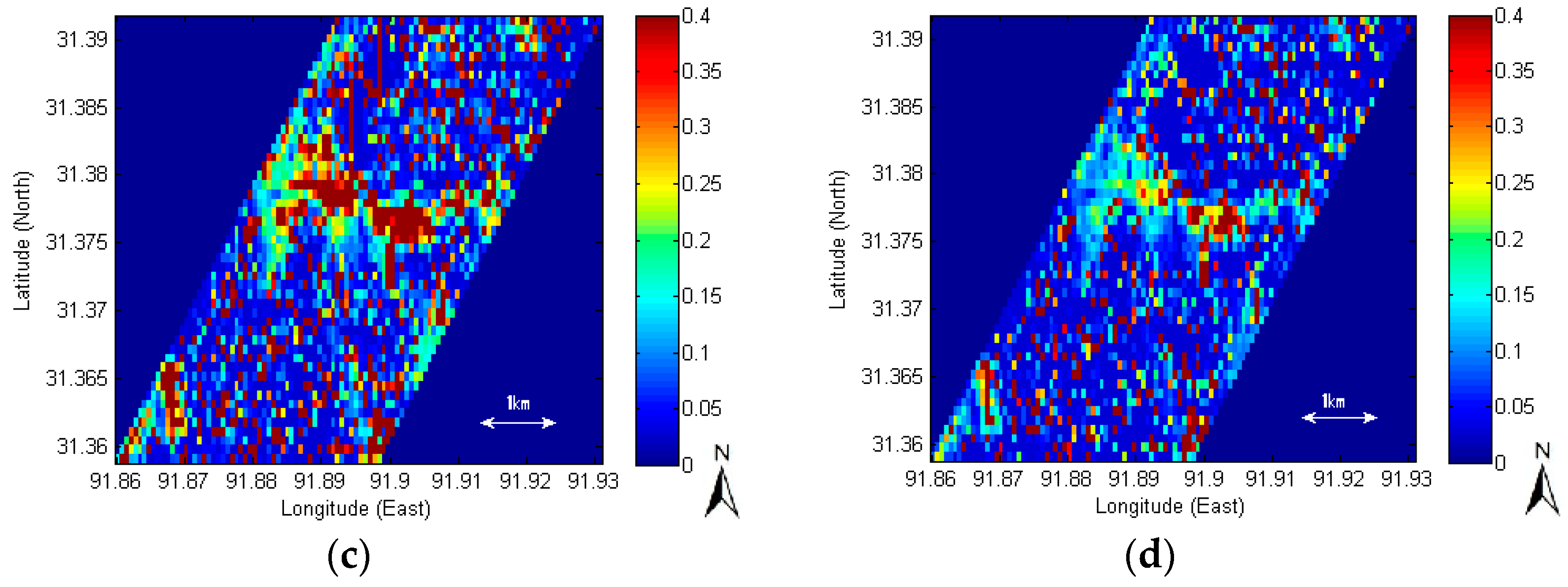
3.2.2. Impact of Backscattering Errors on Soil Moisture Retrievals: Spatial Distribution

The spatial average of the additive backscattering error scheme was higher at 0.1592 m³/m³ than that of the original SAR retrieval (Figure 4a) at 0.1356 m³/m³, while that of the subtractive backscattering error scheme was lower than that at 0.1144 m³/m³. The original SAR backscattering is shown in Figure 4b. The spatial distribution of soil moisture retrieved with the ASAR backscattering hypothetically overestimated by 1 dB is illustrated in Figure 4c, while that of soil moisture hypothetically underestimated by 1 dB is shown in Figure 4d.

In any the ASAR backscattering error schemes, the overestimation of SAR retrievals over the dry area was similarly found, as indicated by several red points in Figure 4c,d. Rather, those overestimations were adjusted by roughness conditions in Section 3.1. Because the original ASAR backscattering measurement (Figure 4b) as well as soil moisture retrieved by the s scheme #4 (Figure 2b) did not show such overestimation over the dry area, in contrast with other roughness conditions in Figure 2a, it was concluded that roughness is mainly responsible for the overestimation in the dry area rather than backscattering errors. From Section 3.1, Section 3.2, and Section 3.3, it was found that the most influential factor in SAR error propagations is roughness, followed by ASAR backscattering overestimation and ASAR backscattering attenuation in descending order [10].

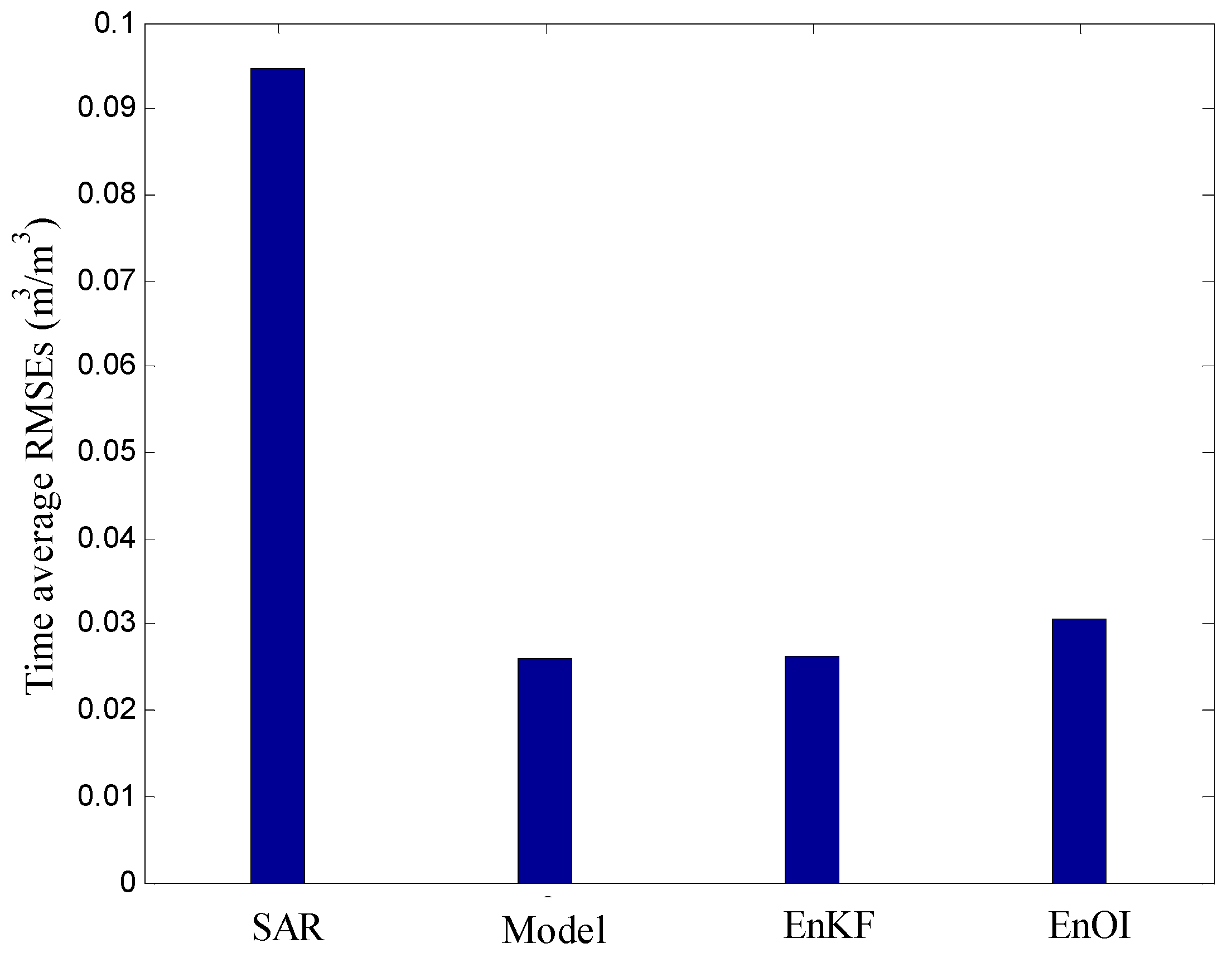
3.3. Validation of SAR Retrievals and Data Assimilation Analysis at a Local Point Scale

In Figure 5, to further assess the SAR errors, the field measurements are compared with SAR, and data assimilation results at a single pixel nearest to a local point station. The SAR overestimation was illustrated to be consistent with discussions above. The EnKF scheme and the EnOI scheme successfully mitigated the overestimation of original SAR retrievals by being diluted with a calibrated model showing the lowest RMSEs.

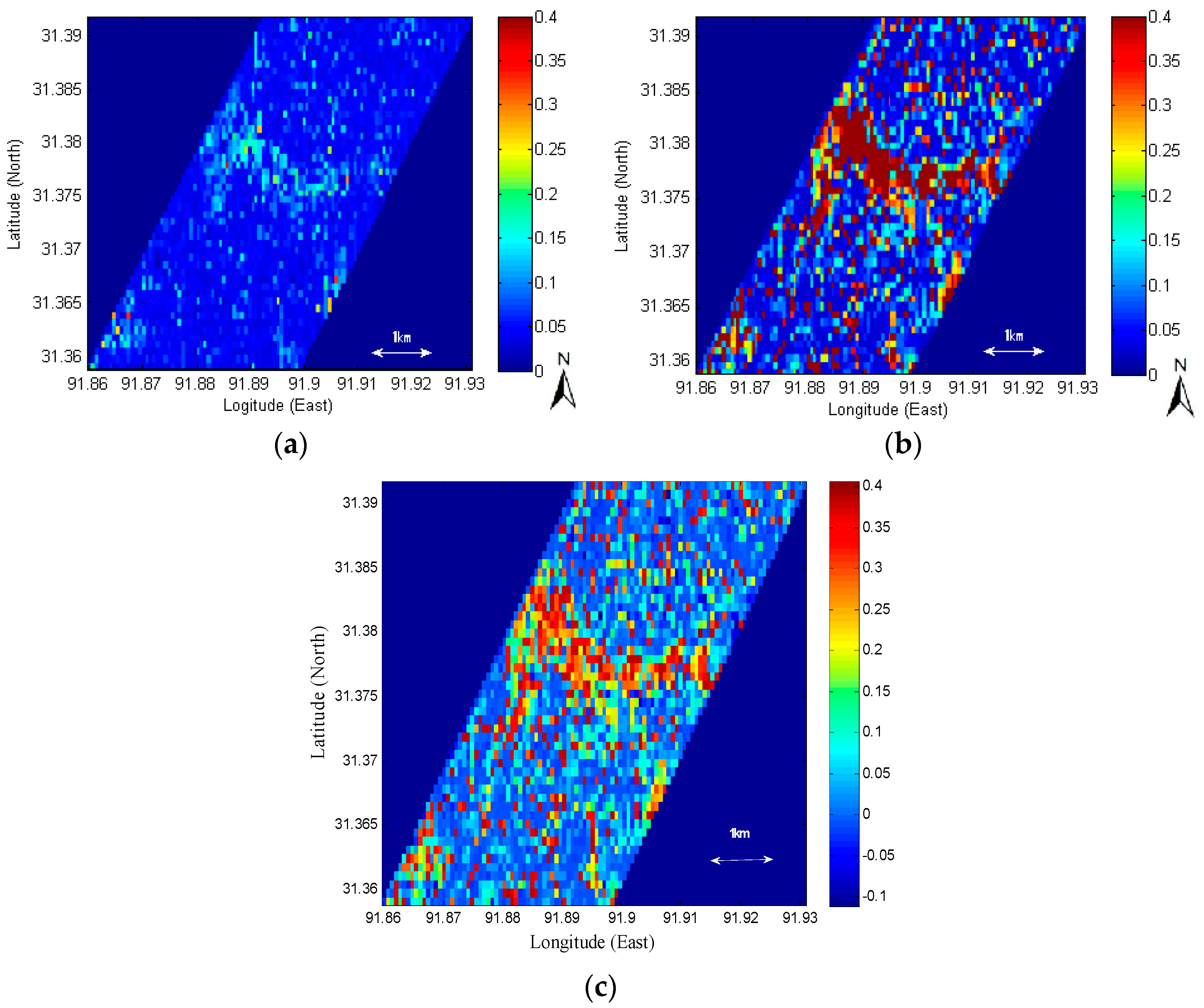
3.4. Spatial Comparison between SAR Retrievals and Land Surface Models

A calibrated model is illustrated in this section to spatially characterize the systematic biases of SAR retrievals. Although the model is the best estimation in Figure 5, the model usually contains uncertainties in input data quality for the spatial variability of rainfall and emissivity, the vertical heterogeneity of subsurface soil and hydraulic properties, or land surface parameterization [32]. However, such model uncertainties were considered to be removed in this study by a calibration, based upon the lowest RMSEs (0.0259 m³/m³) in Figure 5. A detailed calibration scheme was previously provided by [28].

The entire study area was estimated to be mostly dry by a calibrated SVAT model in Figure 6a, while the SAR-retrieved surface soil moisture in Figure 6b was estimated to be much higher than that. The model estimation of those was considered more reliable, based upon the time-average field measurements of soil moisture at 0.0614 m³/m³ during experimental period, and the lowest RMSEs in Figure 5. A spatial average of SAR surface soil moisture was much higher at 0.1140 m³/m³ than that of a calibrated SVAT model at 0.0565 m³/m³. This SAR overestimation in Figure 6b is attributed to the roughness inversion errors. First, the assumption of time-invariance used in Section 2.2.1 as the method for inverting roughness is violated in the event of rain, because the roughness in fact changes due to changes in penetration depth or a film of standing water formed by rain (0.4 mm/d, according to the field measurements). In addition, Figure 2 also supports this. A large difference (model-minus-SAR retrievals) in Figure 6c overlaps with the difference in soil moisture retrievals between Figure 2a,b in Section 3.1 arising from difference in roughness conditions. Based upon consistency between this Section, and Section 3.1, it is considered that Figure 6c further supports the finding that the overestimation of SAR soil moisture is related to roughness.

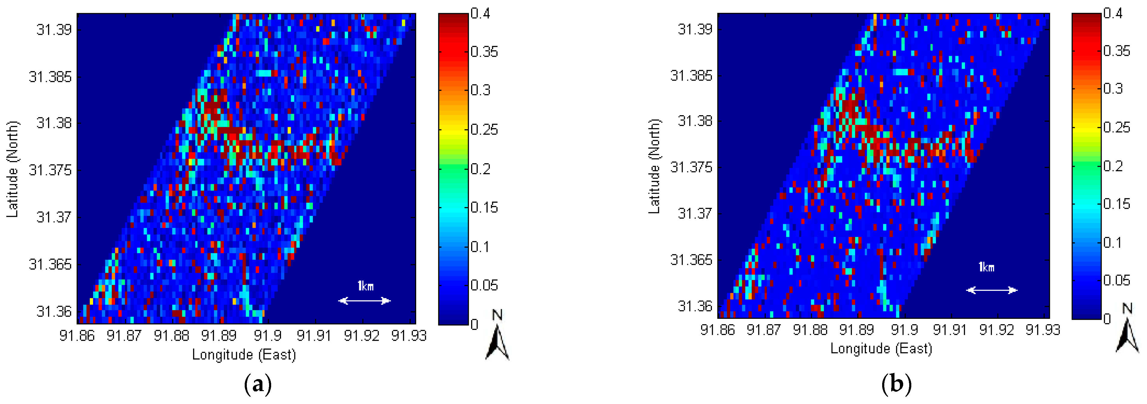
3.5. Spatial Comparison between SAR Retrievals and Data Assimilations

The spatial distributions of EnOI are shown in Figure 7a, while those of EnKF are in Figure 7b. To measure differences in them, the analysis departures (SAR observation-minus-data assimilation analysis, Desroziers et al. [50]) were calculated. The analysis departure of the EnKF scheme was slightly larger at 0.04 m³/m³ than that of the EnOI scheme at 0.03 m³/m³, meaning that the stationary ensemble evolved towards the SAR soil moisture. Figure 8a further shows that both data assimilation schemes successfully provided the intermediate values of spatial averages between two extreme estimates of SAR retrieval and a calibrated model. In specific, the spatial average of the EnOI scheme (stationary ensemble with no time evolution) was lower at 0.1048 m³/m³ than the SAR retrievals at 0.1140 m³/m³. However, it was higher than that of the EnKF scheme (sequential ensemble evolution) at 0.0717 m³/m³ which was closer to a calibrated SVAT model at 0.0565 m³/m³. It was found that a spatial average of the sequential ensemble scheme better reached that of the calibrated model considered as the best estimation in this study. This implies that although the overestimation of the original SAR data were, to some degree, reduced by the stationary ensemble scheme in Figure 7a, there was more mitigation by the sequential ensemble evolution scheme. Thus, it was suggested that the sequential ensemble scheme has a better tolerance to SAR retrieval biases than the stationary ensemble scheme. This difference is due to the ensemble evolution scheme. In Figure 8b, the EnKF made a consistent error reduction, while the EnOI underwent unstable error evolutions. This result is consistent with previous findings that introduced the EnOI scheme as a cost-effective but suboptimal alternative to a sequential EnKF, and that the EnKF scheme outperforms the EnOI scheme [40,51].

This observational error-tolerance of EnKF suggests the operational merits as a satellite data assimilation scheme, as compared to other data assimilations such as a variational data assimilation, optimal interpolation, or stationary ensemble scheme. Because satellite biases still remain even after a satellite bias correction method [40,52], it is an advantage to be tolerant to the observational errors without prior treatments. Although SAR soil moisture retrieval biases may not be completely removed solely with sequential ensemble evolution, it is still more attractive than other data assimilation schemes.

Future research may compare a performance of the 4-dimensional variational data assimilation with that of ensemble Kalman filter with respect to the same SAR observational errors in sub-optimal but more realistic conditions.

4. Conclusions

There is no perfect satellite bias correction method for satellite data assimilation yet, although roughness errors are unavoidable in SAR retrievals. In this context, the impact of the SAR roughness errors on the performance of ensemble data assimilation were examined. To this end, a sensitivity analysis first suggested that the main SAR soil moisture retrieval errors are most likely originated from uncertainty in a priori roughness information. This effect was found larger than vegetation attenuation or other backscattering measurement errors. Next, we also monitored how stationary and sequential ensembles evolve those SAR soil moisture retrieval errors.

The results show that both ensemble data assimilation schemes reconciled the overestimation of SAR data and underestimation of the SVAT model. However, there was a difference in convergence, because of the difference in the ensemble evolution scheme. The spatial average of the sequential ensemble scheme in EnKF was closer to a calibrated SVAT model with the lowest RMSEs, while that of the stationary ensemble was closer to erroneous SAR observations with the highest RMSEs. These results suggest that the stationary ensembles are relatively more vulnerable to SAR retrieval biases than the sequential ensembles that are able to make a self-correction of satellite observational errors. Consequently, this inherent nature of EnKF being more tolerant to satellite biases may suggest operational merits, as compared to other types of data assimilations such as a variational data assimilation or optimal interpolation. Therefore, the needs of each data assimilation scheme for a satellite bias correction may be different.

References

1. Mattia, F.; Satalino, G.; Dente, L.; Pasquariello, G. Using a priori information to improve soil moisture retrieval from ENVISAT ASAR AP data in semiarid regions. IEEE Trans. Geosci. Remote Sens. 2006, 44, 900–912. [Google Scholar] [CrossRef]
2. Verhoest, N.E.C.; de Baets, B.; Mattia, F.; Satalino, G.; Lucau, C.; Defourny, P. A possibilistic approach to soil moisture retrieval from ERS synthetic aperture radar backscattering under soil roughness uncertainty. Water Resour. Res. 2007, 43. [Google Scholar] [CrossRef]
3. Chen, K.S.; Wu, T.D.; Tsang, L.; Li, Q.; Shi, J.; Fung, A.K. Emission of rough surfaces calculated by the integral Equation method with comparison to three-dimensional moment method simulations. IEEE Trans. Geosci. Remote Sens. 2003, 41, 90–101. [Google Scholar] [CrossRef]
4. Fung, A.K. Microwave Scattering and Emission Models and Their Applications; Artech House Publishers: Boston, MA, USA, 1994. [Google Scholar]
5. Lievens, H.; Vernieuwe, H.; Álvarez-Mozos, J.; de Baets, B.; Verhoest, N.E. Error in radar-derived soil moisture due to roughness parameterization: An analysis based on synthetical surface profiles. Sensors 2009, 9, 1067–1093. [Google Scholar] [CrossRef] [PubMed] [Green Version]
6. Ulaby, F.T.; Batlivala, P.P. Optimum radar parameters for mapping soil moisture. IEEE Trans.Geosci. Remote Sens. 1976, 14, 81–93. [Google Scholar] [CrossRef]
7. Huang, C-H.; Bradford, J.M. Applications of a laser scanner to quantify soil microtopography. Soil Sci. Soc. Am. J. 1992, 56, 14–21. [Google Scholar]
8. Van der Velde, R.; Su, Z.; van Oevelen, P.; Wen, J.; Ma, Y.; Salama, M.S. Soil moisture mapping over the central part of the Tibetan Plateau using a series of ASAR WS images. Remote Sens. Environ. 2012, 120, 175–187. [Google Scholar] [CrossRef]
9. Rahman, M.M.; Moran, M.S.; Thoma, D.P.; Bryant, R.; Sano, E.E.; Holifield Collins, C.D.; Skirvin, S.; Kershner, C.; Orr, B.J. A derivation of roughness correlation length for parameterizing radar backscatter models. Int. J. Remote Sens. 2007, 28, 3995–4012. [Google Scholar] [CrossRef]
10. Satalino, G.; Mattia, F.; Davidson, M.; Le Toan, T.; Pasquariello, G.; Borgeaud, M. On current limits of soil moisture retrieval from ERS-SAR data. IEEE Trans. Geosci. Remote Sens. 2002, 40, 2438–2447. [Google Scholar] [CrossRef]
11. Verhoest, N.E.; Lievens, H.; Wagner, W.; Álvarez-Mozos, J.; Moran, M.S.; Mattia, F. On the soil roughness parameterization problem in soil moisture retrieval of bare surfaces from synthetic aperture radar. Sensors 2008, 8, 4213–4248. [Google Scholar] [CrossRef]
12. Draper, C.S.; Mahfouf, J.-F.; Walker, J.P. An EKF assimilation of AMSR-E soil moisture into the ISBA land surface scheme. J. Geophys. Res. 2009, 114. [Google Scholar] [CrossRef]
13. Houser, P.R.; de Lannoy, G.J.M.; Walker, J.P. Land surface data assimilation. In Data Assimilation; Lahoz, W., Khattatov, B., Menard, R., Eds.; Springer-Verlag Berlin Heidelberg: Berlin, Germany, 2010; pp. 549–597. [Google Scholar]
14. Reichle, R.; McLaughlin, D.; Entekhabi, D. Data assimilation using an ensemble Kalman filter technique. Mon. Weather Rev. 2002, 129, 123–137. [Google Scholar]
15. Reichle, R. Data assimilation methods in the Earth sciences. Adv. Water Resour. 2008, 31, 1411–1418. [Google Scholar] [CrossRef]
16. Crow, W.T.; Kustas, W.P.; Prueger, J.H. Monitoring root-zone soil moisture through the assimilation of a thermal remote sensing-based soil moisture proxy into a water balance model. Remote Sens. Environ. 2008, 112, 1268–1281. [Google Scholar] [CrossRef]
17. Dunne, S.; Entekhabi, D. Land surface state and flux estimation using the ensemble Kalman smoother during the Southern Great Plains 1997 field experiment. Water Resour Res. 2006, 42. [Google Scholar] [CrossRef]
18. Hoeben, R.; Troch, P.A. Assimilation of active microwave obser-vation data for soil moisture profile estimation. Water Resour. Res. 2000, 36, 2805–2819. [Google Scholar] [CrossRef]
19. Houser, P.R.; Shuttle worth, W.J.; Gupta, H.V. Integration of soil moisture remote sensing and hydrologic modeling using data assimilation. Water Resour. Res. 1998, 34, 3405–3420. [Google Scholar] [CrossRef]
20. Huang, C.; Li, X.; Lu, L.; Gu, J. Experiments of one-dimensional soil moisture assimilation system based on ensemble Kalman filter. Remote Sens. Environ. 2008, 112, 888–900. [Google Scholar] [CrossRef]
21. Loew, A.; Schwank, M.; Schlenz, F. Assimilation of an L-band microwave soil moisture proxy to compensate for uncertainties in precipitation data. IEEE Trans. Geosci. Remote Sens. 2009, 47, 2606–2616. [Google Scholar] [CrossRef]
22. Margulis, S.A.; McLaughlin, D.; Entekhabi, D.; Dunne, S. Land data assimilation and estimation of soil moisture using measurements from the Southern Great Plains 1997 Field Experiment. Water Resour. Res. 2002, 38. [Google Scholar] [CrossRef]
23. Reichle, R.H.; Koster, R.D. Bias reduction in short records of satellite soil moisture. Geophys. Res. Lett. 2004, 31. [Google Scholar] [CrossRef]
24. Crow, W.T.; Berg, A.A.; Cosh, M.H.; Loew, A.; Mohanty, B.P.; Panciera, R.; de Rosnay, P.; Ryu, D.; Walker, J.P. Upscaling sparse ground-based soil moisture observations for the validation of coarse-resolution satellite soil moisture products. Rev. Geophys. 2012, 50. [Google Scholar] [CrossRef]
25. Lee, J.H.; Im, J. A novel bias correction method for SMOS soil moisture: Retrieval ensembles. Remote Sens. 2015, 7, 16045–16061. [Google Scholar] [CrossRef]
26. Reichle, R.H.; Koster, R.D.; Liu, P.; Mahanama, S.P.; Njoku, E.G.; Owe, M. Comparison and assimilation of global soil moisture retrievals from the Advanced Microwave Scanning Radiometer for the Earth Observing System (AMSR-E) and the Scanning Multichannel Microwave Radiometer (SMMR). J. Geophys. Res. 2007, 112. [Google Scholar] [CrossRef]
27. Ma, Y.; Wang, Y.; Wu, R.; Hu, Z.; Yang, K.; Li, M.; Ma, W.; Zhong, L.; Sun, F.; Chen, X.; et al. Recent advances on the study of atmosphere-land interaction observations on the Tibetan Plateau. Hydrol. Earth Syst. Sci. 2009, 13, 1103–1111. [Google Scholar] [CrossRef]
28. Lee, J.H. Spatial-scale prediction of the SVAT soil hydraulic variables characterizing stratified soils on the Tibetan Plateau from an EnKF analysis of SAR soil moisture. Vadose Zone J. 2014, 13. [Google Scholar] [CrossRef]
29. Lee, J.H.; Timmermans, J.; Su, Z.; Mancini, M. Calibration of aerodynamic roughness over the Tibetan Plateau with Ensemble Kalman Filter analysed heat flux. Hydrol. Earth Syst. Sci. 2012, 16, 4291–4302. [Google Scholar] [Green Version]
30. De Jeu, R.A.M.; Wagner, W.W.; Holmes, T.R.H.; Dolman, A.J.; van de Giesen, N.C.; Friesen, J. Global soil moisture patterns observed by space borne microwave radiometers and scatterometers. Surv. Geophys. 2008, 28, 399–420. [Google Scholar] [CrossRef] [Green Version]
31. Balsamo, G.; Albergel, C.; Beljaars, A.; Boussetta, S.; Brun, E.; Cloke, H.; Dee, D.; Dutra, E.; Muñoz-Sabater, J.; Pappenberger, F.; et al. ERA-Interim/Land: A global land surface reanalysis data set. Hydrol. Earth Syst. Sci. 2015, 19, 389–407. [Google Scholar] [CrossRef]
32. Noilhan, J.; Planton, S. A simple parameterization of land surface processes for meteorological models. Mon. Weather Rev. 1989, 117, 536–549. [Google Scholar] [CrossRef]
33. Noilhan, J.; Mahfouf, J.F. The ISBA land surface parameterization scheme. Glob. Planet. Chang. 1996, 13, 145–159. [Google Scholar] [CrossRef]
34. Lee, J.H.; Pellarin, T.; Kerr, Y. Inversion of soil hydraulic properties from the DEnKF analysis of SMOS soil moisture over West Africa. Agric. Forest Meteorol. 2014, 188, 76–88. [Google Scholar] [CrossRef]
35. Laur, H.; Bally, P.; Meadows, P.; Sanchez, J.; Schaettler, B.; Lopinto, E.; Esteban, D. Derivation of the Backscattering Coefficient σ° in ESA ERS SAR PRI Products; European Space Agency (ESA): Paris, France, 2004. [Google Scholar]
36. Shi, J.C.; Wang, J.; Hsu, A.Y.; O′Neill, P.E.; Engman, E.T. Estimation of bare surface soil moisture and surface roughness parameter using L-Band SAR image data. IEEE Trans. Geosci. Remote Sens. 1997, 35, 1254–1266. [Google Scholar]
37. Ulaby, F.T.; Moore, R.K.; Fung, A.K. Microwave Remote Sensing: Active and Passive Volume II: Radar Remote Sensing and Surface Scattering and Emission Theory; Artech House Publishers: Norwood, MA, USA, 1982; p. 608. [Google Scholar]
38. Su, Z.; Troch, P.A.; de Troch, F.P. Remote sensing of bare surface soil moisture using EMAC/ESAR data. Int. J. Remote Sens. 1997, 35, 1254–1266. [Google Scholar] [CrossRef]
39. Evensen, G. The ensemble Kalman filter: Theoretical formulation and practical implementation. Ocean Dyn. 2003, 53, 343–367. [Google Scholar] [CrossRef]
40. Sakov, P.; Oke, P.R. A deterministic formulation of the ensemble kalman filter: An alternative to ensemble square root filters. Tellus 2008, 60, 361–371. [Google Scholar] [CrossRef]
41. Counillon, F.; Bertino, L. Ensemble optimal interpolation: Multivariate properties in the Gulf of Mexico. Tellus A 2009, 61, 296–308. [Google Scholar] [CrossRef]
42. Lee, J.H.; Pellarin, T.; Kerr, Y. EnOI optimization of SMOS soil moisture over West Africa. IEEE J. Sel. Top. Appl. Earth Obs. Remote Sens. 2015, 8, 1821–1829. [Google Scholar] [CrossRef]
43. Sano, E.E.; Huete, A.R.; Moran, M.S. Estimation of surface roughness in a semiarid region from C-band ERS-1 synthetic aperture radar data. Rev. Bras. Cienc. Solo 1999, 23, 903–908. [Google Scholar] [CrossRef]
44. Escorihuela, M.J.; Kerr, Y.; Wigneron, J.P.; Calvet, J.C.; Lemaître, F. A simple model of the bare soil microwave emission at L-Band. IEEE Trans.Geosci. Remote Sens. 2007, 45, 1978–1987. [Google Scholar] [CrossRef]
45. Barrett, B.W.; Dwyer, E.; Whelan, P. Soil moisture retrieval from active spaceborne microwave observations: An evaluation of current techniques. Remote Sens. 2009, 1, 210–242. [Google Scholar] [CrossRef]
46. Altese, E.; Bolognani, O.; Mancini, M.; Troch, P.A. Retrieving soil moisture over bare soil from ERS 1 synthetic aperture radar data: Sensitivity analysis based on a theoretical surface scattering model and field data. Water Resour. Res. 1996, 32, 653–661. [Google Scholar] [CrossRef]
47. Taconet, O.; Vidal-Madjar, D.; Emblanch, C.; Normand, M. Taking into account vegetation effects to estimate soil moisture from C-band radar measurements. Remote Sens. Environ. 1996, 56, 52–56. [Google Scholar]
48. Bindlish, R.; Barros, A.P. Parameterization of vegetation backscatter in radar-based, soil moisture estimation. Remote Sens. Environ. 2000, 76, 130–137. [Google Scholar] [CrossRef]
49. Scipal, K. Global Soil Moisture Retrieval from ERS Scatterometer Data. Ph.D. Thesis, Vienna University of Technology, Vienna, Austria, 2002. [Google Scholar]
50. Desroziers, G.; Berre, L.; Chapnik, B.; Poli, P. Diagnosis of observation, background and analysis error statistics in observation space. Q. J. R. Meteorol. Soc. 2005, 131, 3385–3396. [Google Scholar] [CrossRef]
51. Oke, P.R.; Sakov, P.; Corney, S.P. Impacts of localisation in the EnKF and EnOI: Experiments with a small model. Ocean Dyn. 2007, 57, 32–45. [Google Scholar] [CrossRef]
52. Anderson, J.L. Exploring the need for localization in ensemble data assimilation using a hierarchical ensemble filter. Phys. D Nonlinear Phenom. 2007, 230, 99–111. [Google Scholar] [CrossRef]
Figure 1. Roughness experiments: a change in relationships between ASAR backscattering and soil moisture retrieved with various RMS height conditions.
Geosciences 06 00019 g001
Figure 2. Roughness experiments: (a) soil moisture retrieval by s scheme #2 (m3/m3); (b) soil moisture (s scheme #4), m3/m3; (c) correlation length, cm; and (d) RMS height (s scheme #4), cm on DoY 221.
Geosciences 06 00019 g002
Figure 3. Backscattering experiments: (a) Relationship between ASAR backscattering with various hypothetical errors and resultant soil moisture retrievals; and (b) the spatial average of the surface soil moisture retrieved with different backscattering error magnitudes used by (a) on DoY 221.
Geosciences 06 00019 g003
Figure 4. Backscattering experiments: (a) soil moisture retrieved from original ASAR backscattering; (b) original ASAR backscattering; (c) soil moisture retrieved from the hypothetical ASAR backscattering error of +1 dB; and (d) soil moisture retrieved from the ASAR hypothetical backscattering error of −1 dB on DoY 221. The unit for (a), (c), and (d) is m3/m3 and the unit for (b) is dB.
Geosciences 06 00019 g004aGeosciences 06 00019 g004b
Figure 5. Time-average RMSEs of surface soil moisture (m3/m3).
Geosciences 06 00019 g005
Figure 6. Surface soil moisture (m3/m3) on DoY 224: (a) Calibrated SVAT land surface model; (b) SAR data; and (c) difference between (a) and (b).
Geosciences 06 00019 g006
Figure 7. Surface soil moisture on DoY 224 (m3/m3): (a) EnOI; (b) EnKF.
Geosciences 06 00019 g007
Figure 8. (a) Spatial average of surface soil moisture (m3/m3); (b) Ensemble evolution of EnOI and EnKF.
Geosciences 06 00019 g008