Abstract
Global Positioning System (GPS) and geodetic control networks are used today for analyzing and monitoring time-dependent crustal deformations, providing a series of accurate positional measurements to deliver information on positional changes and deformations that have occurred. Still, such networks present a low-resolution dispersal of positional measures, and do not take into account various physical constraints that affect the terrain’s seismic behavior. An alternative form of spatio-temporal infrastructure that is feasible and practical to establish might involve the use of Digital Terrain Model (DTM) databases. These databases use higher positional resolutions, and are exhibiting an increasing level of positional and height accuracy. Still, when comparing temporal DTMs, the separation of actual physical phenomena from data-related ambiguities is essential in the framework of spatio-temporal analysis. This paper proposes the use of a hierarchical co-modeling of different DTM databases for the task of landform monitoring. Analyses showed promising results, pointing to the feasibility of the proposed methodology in monitoring and quantifying topographic-related spatio-temporal phenomena, such as landslides and change detection, thus facilitating a reliable and precise landform monitoring and warning framework for geomorphodynamic analyses.
1. Introduction
For the last two decades, permanent Global Positioning System (GPS) and geodetic control networks have been widely used for analyzing and monitoring crustal deformations [1]. These networks provide a series of accurate positional measures that cover the analyzed area, thus providing a time-continuous infrastructure enabling the tracking and studying of landform (seismic, geomorphologic) activities (e.g., [2,3]). A time series of these measures can provide information regarding certain positional changes and deformations that have occurred. Still, these networks present a low-resolution dispersal of positional measures that may encompass dozens and even hundreds of kilometers between two neighboring GPS stations. The entire analysis is therefore based only on discrete distant points, while assuming that the surrounding area, i.e., the GPS station footprint, experienced similar behaviors and trends (e.g., [4,5]). This assumption is not always correct, as different physical constraints, such as geology, may also have a certain effect on the terrain’s seismic behavior. Furthermore, more localized natural disasters, such as landslides or avalanches, will not be detected at all by such monitoring networks. Since developing regions do not always have the means to establish such monitoring systems [6], an alternative form of such temporal infrastructure that is feasible and practical to establish, which still produces qualitative analysis measures, should be considered.
Digital Terrain Model (DTM) databases are perhaps the means for topographic representation most commonly used by the geo-scientific community and are an essential requirement for establishing an efficient and computerized management of our environment. Many National Mapping Agencies (NMAs), as well as private companies and public bodies, are involved today in establishing this type of infrastructure [7]. These DTM databases store sets of spatial positional data in the form of points, lines or surfaces, usually represented in 2.5D, where each planar location within the DTM coverage contains a single height value.
Similarly to GPS monitoring networks, analyzing a time-dependent series of topographic-databases can provide a tool for quantifying changes occurred in the topography, i.e., morphologic landform alterations. GPS networks usually provide a positional observation density of several kilometers at best, while the common nationwide infrastructure DTM databases will usually present a data resolution of a few meters to several dozen meters [8]. Topographic databases having worldwide coverage, like Advanced Spaceborne Thermal Emission and Reflection Radiometer (ASTER) and (Shuttle Radar Topography Mission) SRTM, offer free elevation data that is available on the public domain. ASTER data with a resolution of 30 m (1 arcsec) and height accuracy of 10 to 25 m [9] are available. SRTM is available worldwide at a 90 m (3 arcsec) resolution, with height accuracy of 5 to 10 m [10]. Modern DTM acquisition technologies, such as the TanDEM-X satellite, are designed to produce better worldwide coverage with a resolution of 12 m, with high positional and vertical accuracies (relative vertical accuracy of 2 m) [11]. A comparison of the different characteristics and representations of a time series topography derived from different DTMs can yield a reliable and true-to-nature analysis, i.e., a change-detecting mechanism. Thus, such an analysis can provide an important tool to understand certain natural geomorphologic phenomena, derived from changes in shape and position, and also geodynamic phenomena, derived from deformation and seismic attributes. Consequently, analysis of localized phenomenon is feasible, as opposed to the more general and coarser phenomena presented by the GPS networks. This enables the assessment of certain effects associated with natural disaster occurrences, such as earthquakes, avalanches, and landslides. Another aspect of such an analysis might be establishing an infrastructure that is based on these databases together with specific algorithmic modules in order to monitor and also warn against such unfortunate upcoming events and disasters.
Still, it is commonly the case that the different DTMs used for such monitoring analysis were produced at different times, via different observation technologies (acquisition techniques), presenting different data-structure and datums. These yield global and local irregularities and discrepancies when the DTMs are geographically compared, such that there is a need for a correct and localized mutual modeling of the databases. This increases the potential to identify data-artifacts, which are the result of using different sources, that are not the result of the real physical changes that occurred. Figure 1 depicts such an example, where a direct datum-transformation of two different DTM databases representing the same region cannot resolve supplementary local adjustment required for taking care of morphologic “residuals” still existing, a process that only fine-tuned localized co-modeling can take care of.
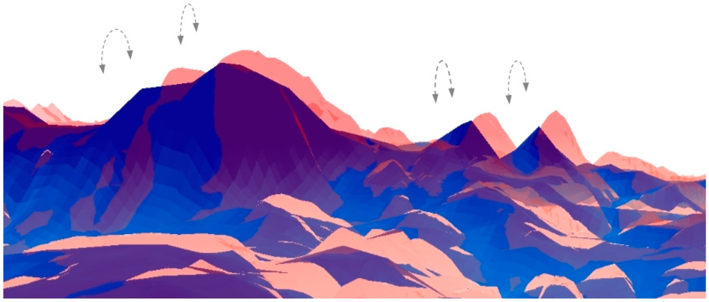
Figure 1.
Direct datum-transformation of two different Digital Terrain Model (DTM) databases showing topographic and morphologic inconsistencies, depicted by arrows, which can be resolved only by rigorous local adjustment.
Figure 1.
Direct datum-transformation of two different Digital Terrain Model (DTM) databases showing topographic and morphologic inconsistencies, depicted by arrows, which can be resolved only by rigorous local adjustment.

This research paper outlines a methodology for hierarchical modeling aimed at solving the abovementioned problem, in which the reciprocal coverage area is divided into homogeneous spatially separate hierarchical mutual-modeling levels. This is meant to produce localized and precise modeling quantification that differentiates between the discrepancies in representations that are the outcomes of the different inner-characteristics each database encapsulates, from actual physical deformations that have occurred, while using the high data level of detail that DTM databases present.
2. Problem Definition
A common assumption is that different DTMs constitute a unique, consistent, uniform, seamless and—as much as possible—homogeneous infrastructure (consistent level of detailing and accuracy, for example). This is a crucial assumption for the implementation of comparison and time-dependent analysis [12]. Until recently, this was true, as these databases were produced via traditional acquisition technologies and production techniques, such as photogrammetry from aerial and satellite imagery or cartographic scanning of existing analogue topographic contour maps. New technologies, such as airborne laser altimetry, i.e., Light Detection and Ranging (LiDAR), have amended this assumption, suggesting non-homogenous infrastructure (data is collected in arbitrary positions with no constant resolution) and recurrent data updates. LiDAR enables high resolution and accuracy in the representation of the observed surface, and the achieved level of accuracy is close to those received by geodetic GPS measurements [13]. LiDAR technology results in data collection and production times that are relatively very fast, enabling quick surface representation in time of crisis and disasters. Together with its high data density and precision, LiDAR technology has great potential for hazard and risk assessment, enabling fast emergency response. Still, time-dependent analyses that make use of such new technologies impose new constraints that need to be addressed, mainly involving the modeling of data as the homogeneous infrastructure hypothesis is no longer valid.
Comparing a time series of different DTM homogenous or non-homogenous databases where each was produced at a different time and via different technology may produce varied accuracy values, level of detail, or data structure, to name a few. Even when no physical changes occurred, these aspects might cause the representations produced via different observation technologies to prove erroneously otherwise [14]. When compared, the representations and positions of the entities described by the different time-dependent databases might show horizontal and vertical geometric discrepancies. These discrepancies affect data-certainty, for example when geomorphologic comparison or change detection processes are at hand. Although direct coordinate-based superimposition comparison of the different databases that is based on the databases’ mutual coordinate reference systems is usually used for such geomorphologic tasks (usually involved to some extent with coordinate-system transformations), it will not suffice in this case and will result in an erroneous topographic analysis [15]. The reality of physical phenomena, which occurred during the acquisition times, adds to the complexity of trying to co-model the observed databases. These factors contribute to the existence of different levels of spatial interrelations of geometric inconsistencies. Investigating these discrepancies and distortions is therefore essential in order to identify and correctly extract changes that did occur; changes which are not artifacts of the representations of the databases compared. Figure 2 depicts near-infrared images of an area that had experienced local landslide, which was a result of an earthquake in the year 2005 near Kashmir, Pakistan [16]. It is quite clear that trying to correlate the 2.5D images is technically very difficult due to distortions in the images, which are the result of the spatial topography and geometry of the terrain and other observation-related effects (e.g., satellite angle and motion) and the lack of mutual geographic coordinates framework. These distortions produce visual offsets in the resulting image that the earthquake did not cause. It is obvious that GPS monitoring networks that were not positioned in this area would not produce any meaningful analysis of the deformation experienced by the topography; a local modeling for such topographic manifestation is therefore essential.
Studies did attempt to investigate the spatial correlations to obtain a complete and continuous model, as in the case of data integration. Feldmar et al. [17] presented a framework for non-rigid surface integration, which ensured a semantic and geometric representation of free-form surfaces, based on global transformation parameters extracted in a matching process. In this case, the authors based their investigation on the assumption that the matched surfaces represent the same object (mostly medically related surfaces); still, in the case of DTM non-rigid surface representation, localized distortions, deformations, multi-qualities, and major displacements are quite common, so the term “same” can become quite ambiguous. Research, such as [18,19,20], has aimed to fuse several DTM databases which were produced via different technologies; all showed that with no prior consideration of DTM datum differences (mostly carried out manually), the terrain representation of the fused DTM was not reliable, sometime even presenting an inferior quality in comparison to any of the source DTM databases. Katzil et al. [21], for example, presented a conflation (“rubber-sheeting”) algorithm using two adjacent DTMs for achieving a more reliable morphological representation of the relief. Together with the abovementioned studies, all proved that when preliminary geometric and topologic adjustments are carried out, the integrated produced DTMs can present a qualitative and reliable surface, in terms of accuracy and morphologic representation.
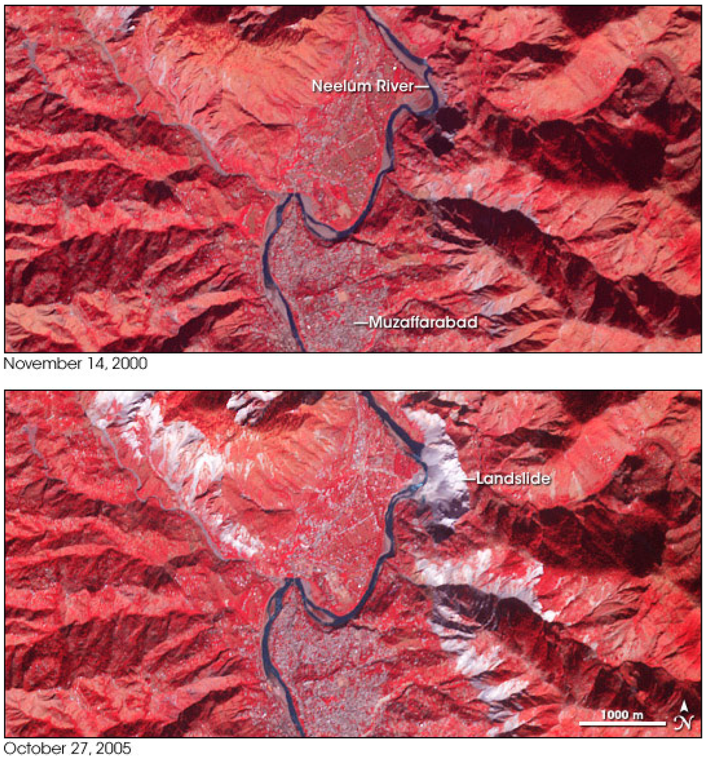
Figure 2.
An area near Kashmir, Pakistan, experienced local landslides in the year 2005: images are made from near-infrared, red, and green light, so vegetation is depicted in red, water in blue, and the effect of the landslide in white or light gray (source: NASA images by Robert Simmon, based on ASTER data).

This manuscript outlines a novel framework for dealing with these problems and considerations. Through specific and designated data-handling procedures, an analysis of the time series data enables the production of qualitative and reliable modeling results. These are used as a monitoring and warning infrastructure for geomorphodynamic terrain phenomena. This framework suggests not relying on a specific global, single and unified modeling structure, but alternatively to “assemble” an infrastructure that is based on (and composed of) several localized ones. This enables more complex and localized geomorphodynamic and monitoring analyses capabilities, such as the calculation of velocity and acceleration attributes. The modeling presented is not dependent on the databases’ data-structure, resolution or accuracy, thus facilitating a reliable and precise landform monitoring and warning infrastructure for geomorphodynamic analyses derived from utilizing a time series of topography representations simultaneously.
The next chapter outlines the methodology regarding the data-handling concept, which is based on a hierarchical modeling of the topographic databases; this is followed by experimental results and analyses of change detection, which are regarded both as artificial topographic changes and natural ones; discussion and conclusions are presented in the closing chapter.
3. Methodology
Modeling, or comparison, of two spatial representations with different time-stamps should provide information on changes that occurred. A series of such models should provide a much more reliable description of local trends and morphologic descriptors, providing a much broader and clearer picture of phenomena that occurred during that time. A comparison modeling mechanism is proposed here, in which the reciprocal coverage area is divided into homogeneous, separate, spatially hierarchical working levels. These are designed for the implementation of mutual spatial registration and matching, thus achieving modeling quantification that differentiate between the discrepancies in representations that are the outcome of different observation technologies and data-structure, i.e., artifacts, and the “real” physical changes that occurred, i.e., deformations. Doing so makes monitoring localized time-related distortions and landform phenomena possible and feasible.
The general time-series modeling methodology is composed of three main processes (summarized below), which are depicted in the block diagram in Figure 3; these are carried out on different data-working levels. The set of these three processes is implemented simultaneously on two databases, while a series of processes is entailed in case more databases are present. The first level has a global form, in which all the data as they exist (i.e., all database points) in the modeled databases are mutually spatially registered (basically, data can be divided into more small areas—such as in the case of nationwide databases—but this is dependent on the amount of data and existing spatial coverage). The second level has a local form, in which all the data are sub-divided into local data-frames, in which mutual spatial matching is implemented on the non-rigid surfaces represented by the databases. This leads to the extraction of local modeling quantifications for mutual data-frames. The overall process can be roughly divided into these stages:
- Global pre-modeling, i.e., registration: relying solely on the databases’ coordinate system might lead to an erroneous comparison quantification. While no implicit information on the spatial correspondence among the topographic databases is present, choosing a common schema (spatial framework) is crucial for non-biased modeling. Registration provides a rough quantification of the modeling discrepancy artifacts. A preliminary registration, or approximate geographic correspondence, of the databases is therefore vital. It is achieved by relying on sets of unique homologous features or objects (geomorphologies) that are identified in the modeled databases. For such a purpose, novel morphologic maxima point identification is developed. The approximate correspondence, which can be expressed by spatial translation, is extracted by constraining a rigid affine spatial transformation-model to selected unique homologous geomorphologic-features, which represent the same real-world object present in the modeled databases. This is a crucial stage when such modeling takes place, more distinctively, when spatial geometric matching process is at hand (e.g., [22,23]). The rigid affine spatial transformation-model is achieved by introducing a constrained ranking of the forward Hausdorff distance mechanism ([24,25]); originally used mainly for image registration, this algorithm was found to facilitate the discrete data representation and was modified to introduce specific constraints to ensure correct solution convergence.
- Local matching: after registration is achieved, a more precise and localized matching of databases can take place, which aspires to locally fine-tune the global registration quantification extracted. Matching of spatially continuous entities is usually based on geometric or conflation schema specifications analyses, while algorithms implemented are mainly dependent on the geometric types of the objects needed to be matched, their topological relations, their data volume and the semantics of attributes [26]. A robust and qualitative matching process suitable for the data characteristics present is the Iterative Closest Point (ICP) algorithm [27]. The ICP algorithm is designed for matching 2D/3D curves and rigid surfaces using nearest neighbor criteria. The implementation carried out here utilizes an iterative Least Squares Matching (LSM) process [28], with specific geometric constraints and optimizations tailored for this task [29]; these are intended to achieve a faster convergence, but mainly to overcome constraints and characteristics the non-rigid data impose (landform representation). The a priori corresponding registration value extracted on the global, i.e., higher, working-level is used for initialization of this process. By dividing the entire mutual coverage area into homologous separate frames and implementing the ICP matching process on each of these frames separately, better localized modeling—and hence monitoring—is feasible. This enables more accurate categorization of local phenomena instead of an ambiguous global one, such as the outcome of the footprint effect related to GPS monitoring network.
- Analysis and comparison of time-series databases: the outcome of the local ICP matching process leads to the establishment of a mutual-modeling structure, similar to a 2D matrix. Each cell in this matrix stores the accurate local spatial matching rigid-model quantification (i.e., parameters) that corresponds to each of the local mutual frames matched. By inspecting these quantifications—statistically and with respect to their surroundings—one can identify the deformations and distortions the local landform had experienced. Since the artifact discrepancies are known and modeled, the actual geomorphologic changes that occurred can be precisely and more easily modeled and understood.
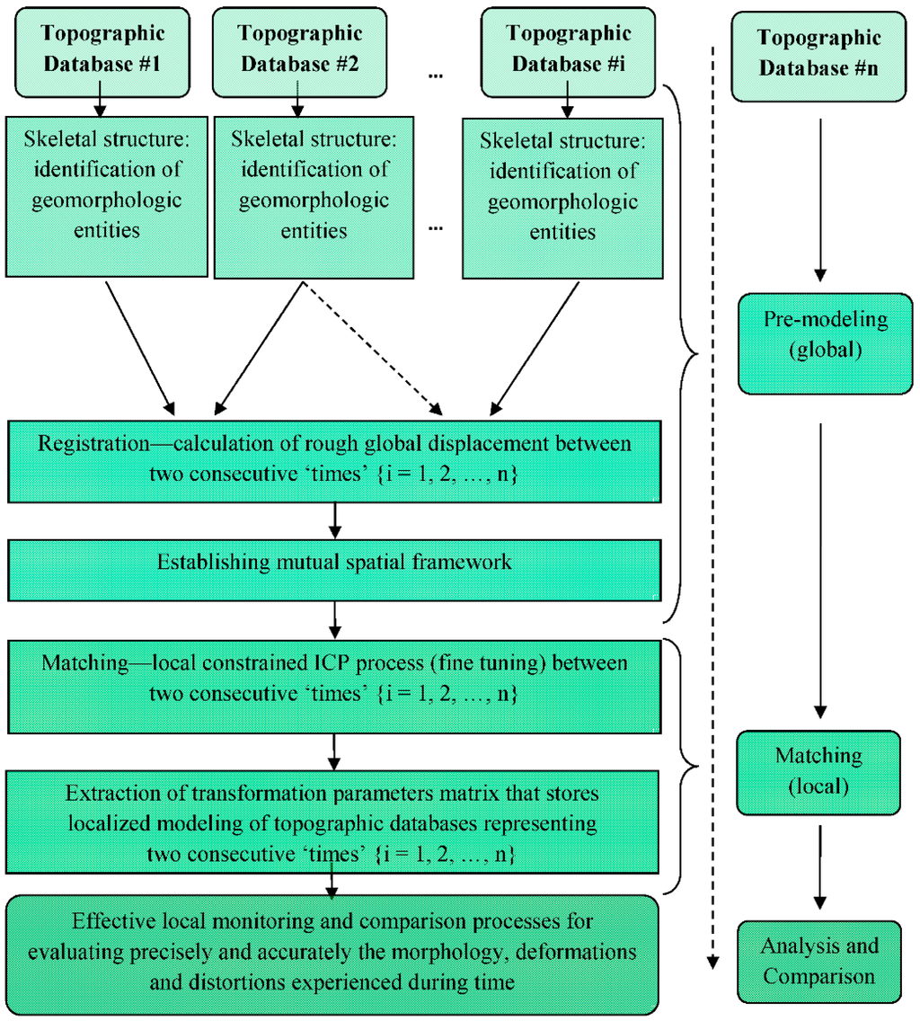
Figure 3.
Block diagram of the proposed time-series hierarchical comparison methodology.
Figure 3.
Block diagram of the proposed time-series hierarchical comparison methodology.

3.1. Global Pre-Modeling
3.1.1. Identification of Unique Geomorphologic Entities
Relying on distinct entities that exist and are represented in the different databases should overcome geometric ambiguities in data-modeling and provide a more reliable quantification of the databases’ spatial correspondence. Unique entities, such as interest points on the surface, provide information regarding the skeletal structure of the topographic database. Certain features in the topography have unique geomorphometry that differentiate them from their surroundings, such as areal features; for example, basins and hills. These features have certain surface descriptive attributes, defined by specific geometry and topology, which can be identified by local differences in elevation values, i.e., local elevation extreme. Characterizing a peak in the height values is relatively easy to categorize, but still, the identification of peaks should be treated more globally, not locally. This means that relatively wider surroundings should be chosen around a point suspected to be a peak in order to categorize it as one. This is vital in order to reject local peaks that can be related to a small abruption in the topography, as well as to incorrect modeling or errors and noise. This means that only peaks with some significant amount of topographic prominence or horizontal topographic isolation (distance from the nearest point of higher elevation) should be considered as maxima points. These global maxima give a good perception of the skeletal structure of the terrain [30]. Since databases exist with different resolution and accuracy values, which affect the definition and existence of morphologic features in the topographic representation, a rigorous and robust analytical definition of topographic global maxima features is required. Nevertheless, an assumption can be made that due to the large coverage extent of topographic databases (at least hundreds of square kilometers), a large number of such entities will exist in all analyzed databases (as long as the landscape represented is not flat; in this case, co-modeling of topographies is not always possible).
Finding global maxima is the goal of optimization. If a two-dimensional function is continuous in a closed interval, then by the extreme value theorem global maxima exist. This theorem states that if a real-valued function f is continuous in the closed and bounded interval [a, b], then f must attain its maximum at least once [31]. That is, there exist numbers c and d in [a, b], depicted in Equation (1), such that:
Furthermore, global maxima must either be local maxima in the interior of the domain, or must lie at the boundary of the domain. So, a method of finding global maxima is to look at all the local maxima in the interior and also to look at the maxima of the points on the boundary and choose the largest value of them all.
The three-dimensional terrain surface is a complex shape, so it is impossible to use any mathematical function to completely describe it. Alternatively, assigning interpolation functions can be used in order to approximate it, which consequently introduces accuracy errors. Utilizing local surfaces is usually how this is solved. The idea behind the best-fitting concept is to treat small surface variations as highly complex, so they can be treated as a stochastic process [32], while for best-fitting of local surfaces the use of least-squares is suggested. In the case of curved surfaces, as in terrain surface representation, the common functions used are the second-order and third-order polynomials or bi-cubic functions (for 2D and 3D data-types, respectively), based on linear adjustment of the data, as in Figure 4.
Based on the aforementioned, a novel computational approach is devised, aimed at correctly defining these unique points that define the skeletal structure of each DTM database, which are the basis for the registration process. The approach includes:
- The computation of four best curve-fitting (2D space) orthogonal second-degree polynomials, one for each principal orientation, from all DTM points that exist in the data. Since resolution affect the topographic representation, a sensitivity analysis was done, which showed that the number of points required for defining the polynomial has to be at least 200 m for each principal orientation; for example, in a 50 m grid, 4 points are needed. The assumption is that such coverage area ascertains the identification of local maxima in the topography (see Figure 5);
- The calculation of the integral (area) of the four best-fitting polynomials in the z direction relative to the height of the farthest point in the polynomial with respect to the examined DTM point;
- Statistical thresholds tests of polynomials’ coefficients and integral values to examine the polynomials’ topological behavior (e.g., ascending or descending, magnitude with respect to surroundings);
- Local clustering via distance-measure on all previous identified maxima points (depicted as red points in Figure 5) aimed at finding an area-of-interest; distance value used for clustering equals to the grid interval value;
- Local bi-directional interpolation within each cluster (depicted in Figure 5) to ensure the precise calculation of the highest topographic location (depicted as blue point), thus achieving planimetric sub-resolution accuracy.
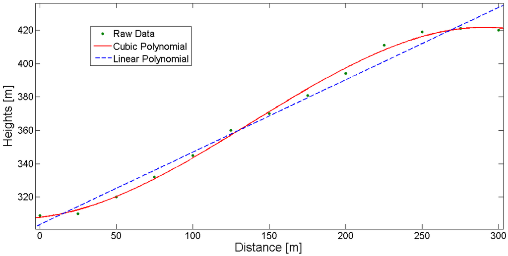
Figure 4.
Best-fitting linear and cubic polynomial for given height data (section view).
Figure 4.
Best-fitting linear and cubic polynomial for given height data (section view).

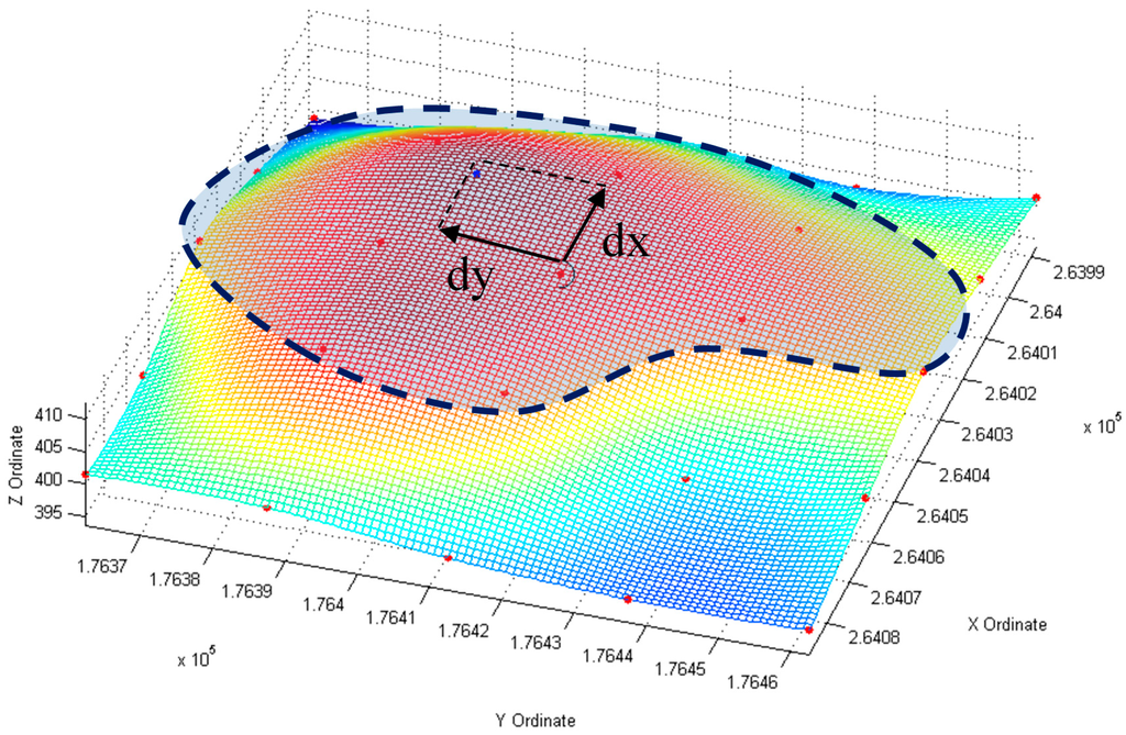
Figure 5.
Clustering (dashed polygon) and local interpolation (depicted with dx and dy) around cluster-maxima for the identification of the precise position of interest point (blue point).
Figure 5.
Clustering (dashed polygon) and local interpolation (depicted with dx and dy) around cluster-maxima for the identification of the precise position of interest point (blue point).

3.1.2. Registration
Registration of DTM databases can be categorized based on feature-based registration, in which one is the reference while the other is the target. A registration process searches for the best fit for the two, where a spatial transformation enables the target to align with the reference. The correspondence between features enables the calculation of the transformation and thus establishes feature-to-feature correspondence between the reference and target [33]. The transformation is global in nature, such as a gross error, so it cannot model local geometric differences between the models registered.
The problem at hand suggests a different data-structure for the time-series databases, and different data coverage, together with the fact that the different topographic databases might present global as well as local distortions, with different levels of detail, resolution and sensitivity to computed terrain attributes. This translates to a dispersal of the two sets of interest points seen to be different, together with the existence of data outliers. Consequently, an absolute singular minimal mismatch value (such as the one computed via the Hausdorff distance, e.g., [24]) is not certain. Thus, certain constraints are added here to ensure the best matching extraction, i.e., introducing partial distance voting criteria that are based on a ranking process [25]. The ranking is based on the highest ranked point of B by the distance to the nearest point of A, which is not specifically the largest distance that exists. This means that, S of the c model points (1 ≤ S ≤ c) is given by taking the Sth ranked point of B, rather than the largest ranked one, as suggested in Equation (2).
where Sth denotes the ranked value in the set of existing distances, while ranking is achieved by the perspective values of this distance. Thus, the “best matching” is chosen by identifying the subset of the model that minimizes the direct Hausdorff distance (hs).
3.2. Local Matching
The matching and modeling of DTM databases or topographic surface-models is rarely addressed directly in the literature; adapting existing matching algorithms to this task, for example from the Image Analysis or Computer Graphics disciplines, is feasible. A robust and qualitative matching algorithm of two spatial shapes, named ICP, is presented in [27]. ICP is a 2D/3D transformation model extraction that establishes an iterative process for the identification and coupling of counterpart points: source-to-target (g(x,y,z) ⇒ f(x,y,z), correspondingly), which are the closest that exist. The algorithm estimates similarity transformation parameters between the spatial databases, or non-rigid surfaces, minimizing the Least Squares differences along the z-axes.
Target-point that does not exist in the data but upholds the continuous function of the target-surface will ensure the closest point definition. Consequently, a nearest-neighbor search criteria process with designated geometric and computational optimizations [29] that uses perpendicularity of point-to-surface geometry constraints for locating that point, either grid or triangular, is implemented. The schematics of an ICP process on DTM grid structure are depicted in Figure 6 and Equation (3) (certain minor modifications are required for non-grid data-structures, i.e., a triangular domain, whereas the schematics of the ICP are depicted in Figure 7).
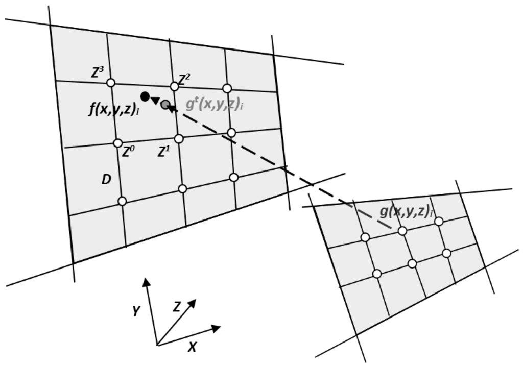
Figure 6.
Schematic explanation of least squares target function minimization via perpendicularity constraints in grid-domain, ensuring closest point.
Figure 6.
Schematic explanation of least squares target function minimization via perpendicularity constraints in grid-domain, ensuring closest point.

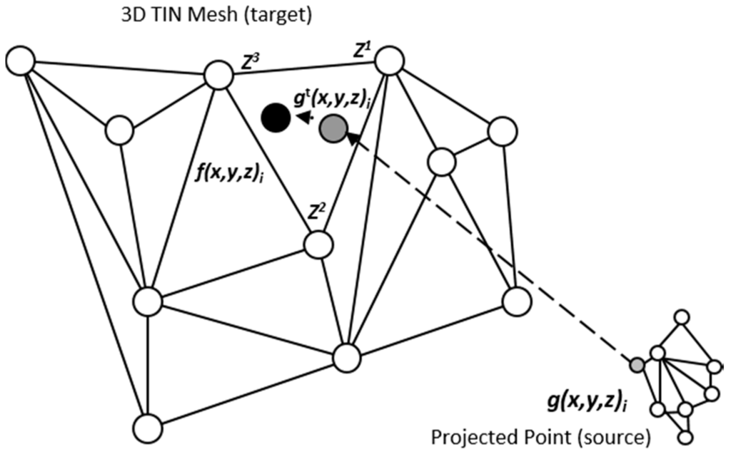
Figure 7.
Schematic explanation of least squares target function minimization via perpendicularity constraints in TIN triangular-domain, ensuring closest point.
Figure 7.
Schematic explanation of least squares target function minimization via perpendicularity constraints in TIN triangular-domain, ensuring closest point.

3.3. Analysis and Comparison
Based on the assumption that inherent local discrepancies exist between the topographic databases, it is clear that small zonal data-frames should be fitted much better and more accurately than large ones. Hence, the matching process should introduce approximately the same topographic matching values in neighboring frames. This enables monitoring of local anomalies or distorted matching processes—according to their values, which point to deformations and distortions the modeled landscapes had experienced. In other words, the change detection assumption is that all mutual frames should be matched accurately and with roughly the same transformation (matching) values (which should be in the locality of the used global registration values), except for the frames affected by the monitored landform phenomena. As a result, the spatial modeling quantification should be continuous in value over the entire area—except for the regions suspected to have experienced landform deformations. This is in contrast to large and biased variations and truncated values that are the consequence of modeling large frames, which also lack the possibility of modeling local phenomena and distortions. The more unified the values are, the more reliable the error vector e(x,y,z) of the ICP LSM process, i.e., better mutual spatial correspondence, whereas large variants indicate larger values and anomalies of this error vector, e.g., modeling irregularities.
Other than the values themselves, other statistical estimators can be used, for example the number of corresponding point-pairs included in the ICP process and solution, or the number of iterations required for its convergence. All these contribute to a more reliable analysis that enables a local and precise quantification.
Each matching set in each frame includes the transformation parameters that best describe the relative spatial geometry of the mutual homologous frames that were matched. These sets can be described as elements stored in a 2D matrix: each set is stored in the cell that corresponds spatially to the frames that models their mutual correspondence, as depicted in Figure 8, and represents the results extracted by a single independent local ICP process. This data structure contributes to the effectiveness of the modeling, monitoring and comparison processes that need to be carried out locally in order to evaluate the analyzed morphology more precisely and accurately. A statistical and/or visual examination of the values stored in the matrix can give information and quantification regarding certain morphological changes and geometric anomalies that occurred along the time-series modeled by the series of DTM databases—or are still occurring.
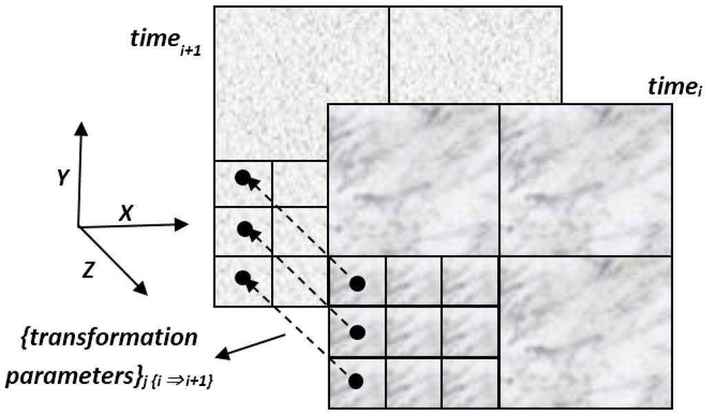
Figure 8.
Topographic databases with times i and i + 1 (front and background). Each matrix-cell {j} in i stores a set of corresponding transformation parameter that best describe the relative spatial geometry of the mutual homologous topographic frames i + 1 that were matched in the Iterative Closest Point (ICP) process.

4. Experimental Results
4.1. Validation
4.1.1. Interest Point Identification
Perhaps the simplest and still reliable verification method of interest point identification can suggest a visual examination. Figure 9 depicts two examples (Central Galilee region, Israel) showing precise identification of topographic maxima. Red sections depict areas-of-interest, while a maxima (single position) is identified for each.
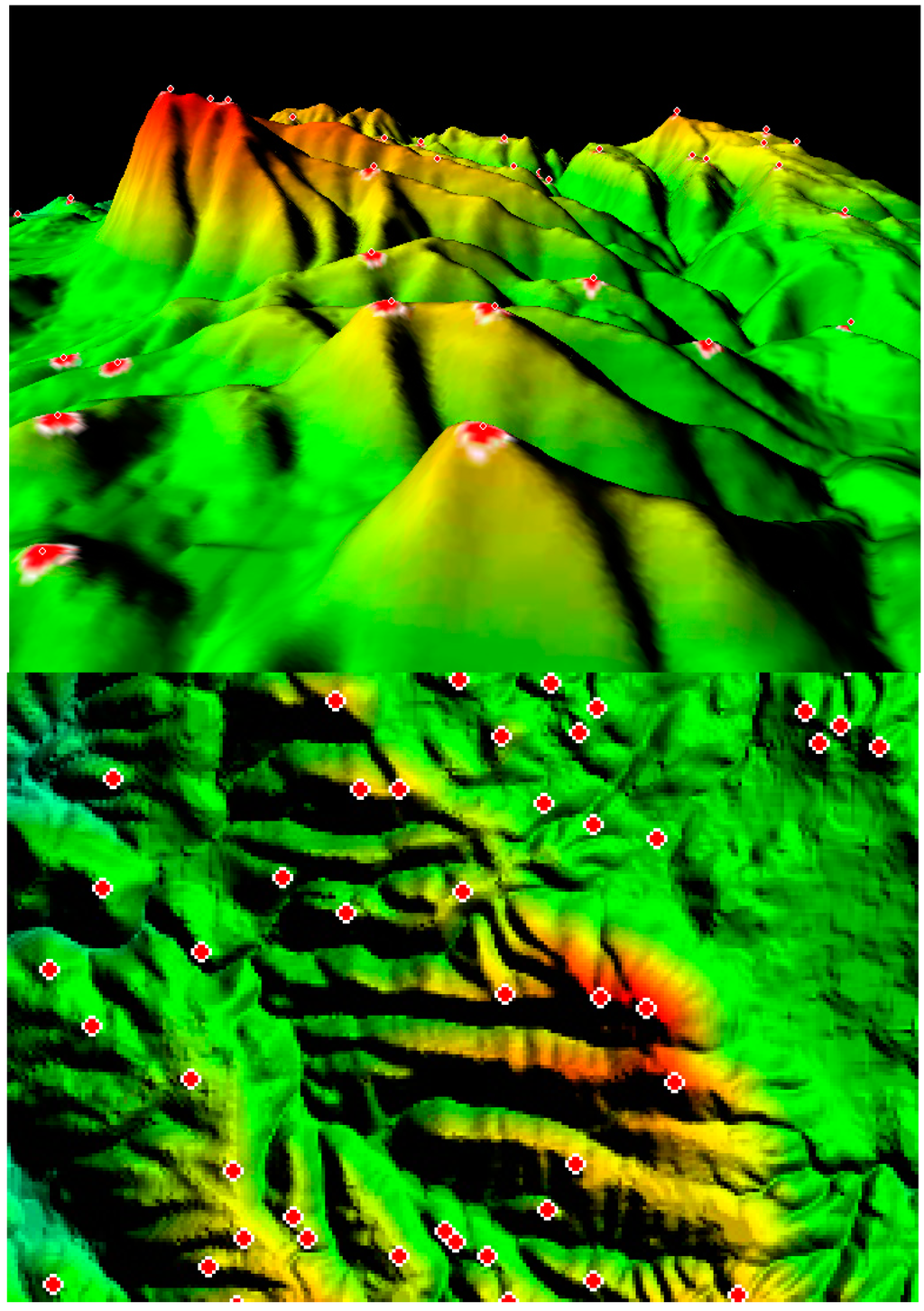
Figure 9.
3D (up) and 2D (bottom) visualization of interest point identification superimposed on the topography.
Figure 9.
3D (up) and 2D (bottom) visualization of interest point identification superimposed on the topography.

When the skeletal structures of different databases representing the same area are compared, different point distributions and positions are evident; this is logical due to the fact that the processed databases have different data-characteristics, namely level of detail, resolution, morphological representation, to name a few. Still, the assumption that homological points exist, which represent the same feature in reality, is validated (depicted in Figure 10).
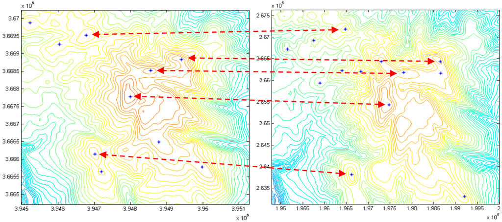
Figure 10.
Height contour representation of the topography superimposed with the interest points identified for each database; corresponding interest points are shown.
Figure 10.
Height contour representation of the topography superimposed with the interest points identified for each database; corresponding interest points are shown.

4.1.2. Registration
To evaluate the effectiveness of the registration algorithm, a synthetic numerical analysis was implemented, in which an area was cropped from a DTM, then registered back into the original DTM. Before registration, the coordinates of the cropped DTM were spatially displaced with values of {tx, ty, tz} = {125, −50, 30} m. Vertical arbitrary noise shifts were also added to the cropped DTM z-values, with values of −30–+30 m, with a mean value of 0 m. The cropped area covered approximately 25 km2, having 32 interest points, while the original DTM covered 100 km2, having 170 interest points. It is important to note that not all interest points in the cropped area were also identified in the larger area original DTM, proving that the displacement and noise had an effect on the interest point identification algorithm.
The differences between the calculated planar registration values and the used values are given in Table 1. These are satisfactory, due to the fact that the noise factor that was added in this analysis was in the range of several dozens of meters, while the resulting Standard Deviation (SD) in both axis directions was less than 5 m. This proves that this algorithm is robust and accurate in identifying a single global registration value, despite datum differences, massive translation and the existence of noise factors.

Table 1.
Statistical numerical values of the proposed registration algorithm carried out on synthetic data (values in meters).
| Parameter | Used Value | Value Calculated | Value Difference | Value Standard Deviation (SD) |
|---|---|---|---|---|
| tx (m) | 125 | 124.6 | −0.4 | ±3.2 |
| ty (m) | −50 | −50.4 | −0.4 | ±2.8 |
4.1.3. Matching
A synthetic point cloud was generated, which contained close to 8000 points. The point cloud was then transformed with these 6-parameter transformation values: {tx, ty, tz} = {1.2, 1.0, 2.5} m and {φ, κ, ω} = {2.0, 1.0, 0.0} decimal degrees. First, the entire area was matched in a single process, resulting in the 6-parameter transformation values depicted in Table 2. These values verify that the entire constrained ICP process is correct, while producing accurate and reliable results. The number of registered points for the entire area was more than 90% out of all available.
Table 2.
Statistical numerical values of the Iterative Closest Point (ICP) process on point clouds (covering approximately 100 m2).
| Parameter | Value Used | Value Calculated | Value Difference |
|---|---|---|---|
| tx (m) | 1.200 | 1.207 | 0.007 |
| ty (m) | 1.000 | 0.998 | 0.002 |
| tz (m) | 2.500 | 2.497 | 0.003 |
| φ (decimal degrees) | 2.000 | 1.925 | 0.075 |
| κ (decimal degrees) | 1.000 | 0.988 | 0.012 |
| ω (decimal degrees) | 0.000 | 0.031 | 0.031 |
A second numerical analysis was carried out, in which the entire coverage area (XY plane) was divided into four partially overlapping frames. Each frame was then matched independently and separately. The corresponding four groups of computed 6-parameter transformation values are superimposed on the frames depicted in Figure 11. The computed three translations are in the range of a few centimeters from the actual used values for the performed transformation. The computed rotation values are in the range of several degrees from the actual used values for transformation (though in most cases the differences are less than 0.5 degrees). This can be explained by the fact that these values are computed with respect to the center-of-mass of each frame, while the rotation itself in the original transformation was carried out with respect to the center-of-mass of the entire model. While one decimal degree translates here to 4 cm for the farthest point (radius of 2.5 m for each frame), this difference in magnitude still represents an accurate result. Moreover, each frame introduces different geometry and dispersal of data, thus contributing to different calculated transformation values. Nevertheless, by observing the computed values, it is clear that they are continuous and generally consistent in value for all four frames, thus suggesting an adequate and reliable solution.
4.2. Morphological Analysis
4.2.1. Landslide Analysis
Landslide detection and quantification numerical analysis was evaluated via the proposed methodology. DTM covering 25 km2 with 25 m resolution was chosen as a reference representing the area of Mount Carmel ridge in the north of Israel. The ridge itself is situated on relatively active faults. A LiDAR scan with a density of approximately 0.2 points per 1 m2 was used as subject for the evaluation of landform changes. The LiDAR scan covers an area of approximately 4 km2 on the southeast side of the reference DTM with approximately 800,000 points (representing a density of more than 120 times the reference within the mutual coverage area). The DTM production time is 20 years earlier than that of the LiDAR.
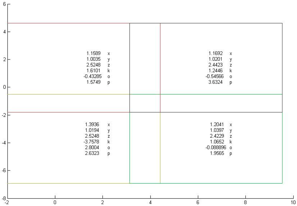
Figure 11.
Computed ICP matching process transformation values for each frame.
Figure 11.
Computed ICP matching process transformation values for each frame.

A landslide simulation based on a 3rd degree polynomial was implemented on the LiDAR model on the south-east side of the ridge, covering an area greater than 400 by 600 m. The simulation modeled here was categorized according to zones that corresponded morphologically with large shear strains—approximated by two straight lines (top and bottom)—corresponding to the steep slip surface. This landslide’s failure mechanism can be classified as a “generalized translation failure”, where the critical clip surface is a single straight line with deep or shallow failure [34]. The maximal height change in the displaced area (depletion zone) was approximately −30 m, while the maximal height change value in the accumulated debris area (accumulation zone) was approximately 40 m. A noise factor of approximately ±1 m was added to each LiDAR point height that was affected by the landslide simulation. A comparison of both topographies with a view from the ridge—before and after—is depicted in Figure 12.
The assumption is that during the matching process, all mutual frames should be matched with a relatively similar matching quantification—a transformation value that is a result of datum discrepancies, except for the frames affected by the landslide phenomena—a transformation value that is a result of physical changes. As a result, the spatial translation (tx,ty,tz) should be relatively close to the initial registration vector used in each independent ICP process, i.e., being continuous in value over the entire area, except for the landslide region. Figure 13 depicts the landslide data (LiDAR topography) superimposed on the DTM data, clearly showing the morphologic changes occurred within the landslide-affected area (while the depletion zone is not visible), with some minor changes in the vicinity, which can be considered natural morphologic changes over time.
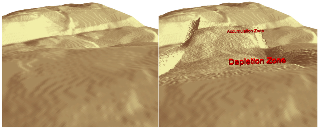
Figure 12.
Shaded relief representation (view from the ridge) of the landslide simulation on subject Light Detection and Ranging (LiDAR) data: before (left) and after (right).
Figure 12.
Shaded relief representation (view from the ridge) of the landslide simulation on subject Light Detection and Ranging (LiDAR) data: before (left) and after (right).

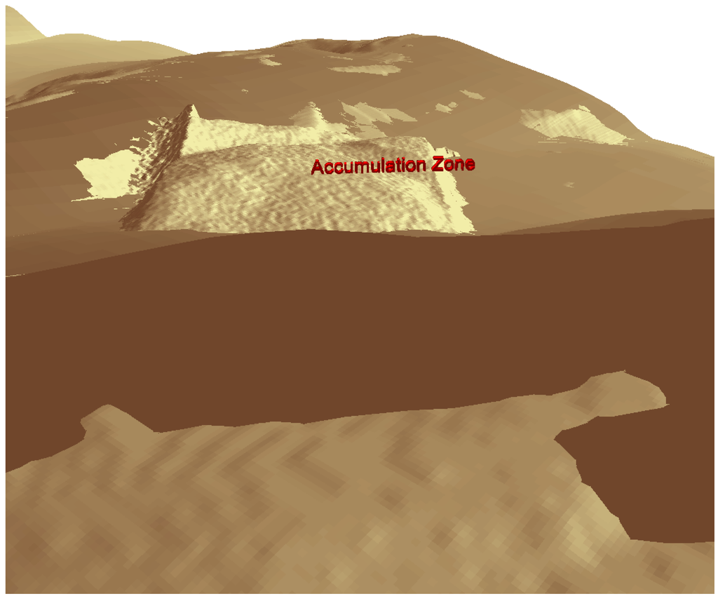
Figure 13.
LiDAR topography superimposed on the DTM topography.
Figure 13.
LiDAR topography superimposed on the DTM topography.

Figure 14 shows the results obtained while using the proposed mechanism of hierarchical registration and matching (left column), compared to the straightforward coordinate-based comparison (right column); the area that experienced the landslide is circled. The top row depicts the 2D displacement vectors for each small area (a frame covering approximately 100 m2) matched in the ICP. It is evident that when using the registration quantification calculated in the ICP (left-hand side) the results are more uniform and have the same trend, depicted as arrows; the only area that shows some irregular values is the area suspected to experience the landslide. When no preliminary value is used for matching (right-hand side), the displacement vectors change with no apparent trends, evidently showing noise with no clear matching correspondence or evident trend. Bottom row depicts the 3D displacement vectors for each small area matched in the ICP. Again, left image shows small displacement values—except for the area suspected with landslide, where vectors point to directions that encountered massive morphologic changes. The right image depicts noise with no clear matching, which makes the identification of the landslide and its magnitude very hard.
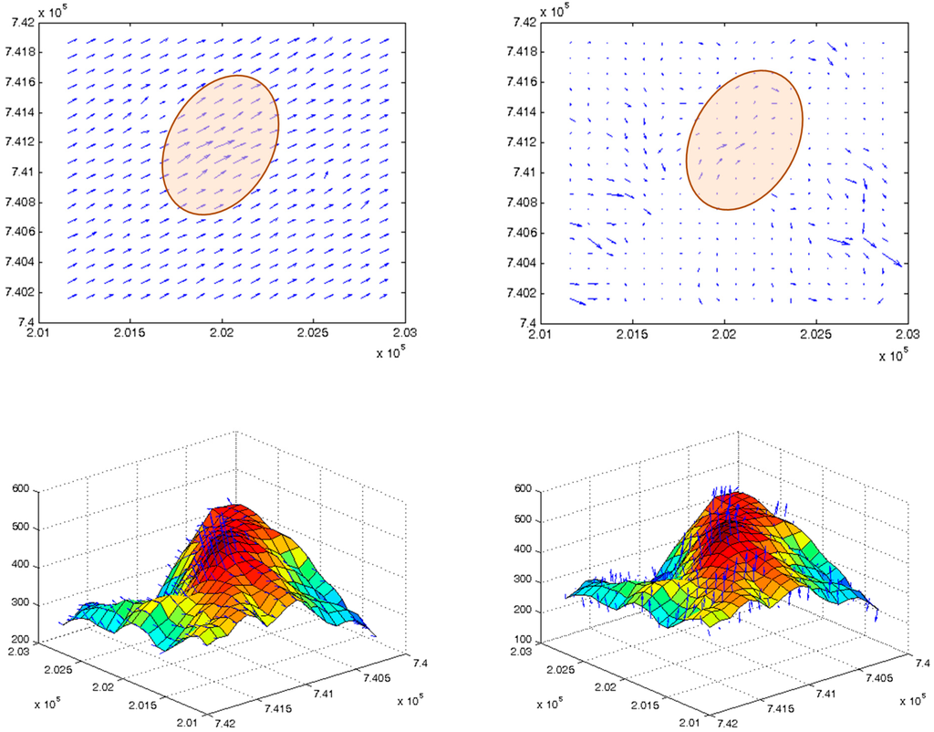
Figure 14.
Landslide detection: results received by using the proposed mechanism of hierarchical registration and matching (left), and results received via the straightforward coordinate-based comparison (right).
Figure 14.
Landslide detection: results received by using the proposed mechanism of hierarchical registration and matching (left), and results received via the straightforward coordinate-based comparison (right).

A better numerical quantification can be extracted by inspecting the displacement of the dz values for each matched area, depicted in Figure 15. Again, it is clear that via the proposed hierarchical modeling (left) the area encountered with landslide is easily visible, together with values of vertical displacement; the rest of the area shows a vertical displacement of close to zero (meters), suggesting good correspondence between local surfaces, with minor value changes that can be explained by local minor morphological changes (such as new roads, structures or hydrologic streams created during time). On the right image it is quite hard—almost impossible—to identify the area suspected to have encountered the landslide, which is a result of no preliminary modeling pre-processing, namely spatial registration. These figures illustrate the significance of prior registration to the ICP processes and that both these processes have an essential role in ensuring a correct and accurate modeling for landslide modeling processes or any other natural phenomena. This is in contrast to a direct superimposition process that does not use the geometric inter-relations of the two models. Thus, the extraction of a mutual geospatial framework is mandatory. Without preliminary registration, extracting the spatial artifacts from the real displacements is almost impossible to accomplish—mainly within the horizontal domain.
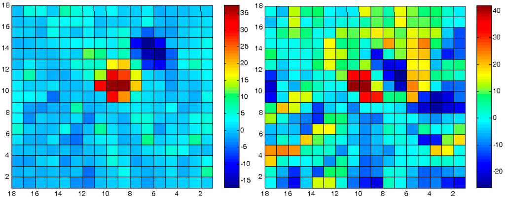
Figure 15.
dz displacement values for matched frames—proposed hierarchical mechanism (left), and straightforward coordinate-based superposition (right). Values are in meters.
Figure 15.
dz displacement values for matched frames—proposed hierarchical mechanism (left), and straightforward coordinate-based superposition (right). Values are in meters.

Moreover, in case each the database has a time-stamp—for example (just) before and (just) after the landslide occurred—these displacement vectors could easily be translated and quantified to the velocity and acceleration changes each zone in the analyzed topography had experienced, enabling research with a much more complex and accurate spatio-temporal geomorphodynamic resolution.
4.2.2. Change Detection
The proposed methodology was analyzed to assess its feasibility in identifying localized change detection in a spatial scene. LiDAR and gridded DTM databases were analyzed, having different levels of detail and data structures with a mutual coverage area of approximately 3 km2, depicted in Figure 16. Within the mutual coverage area, the DTM had less than 3800 points, with the LiDAR representing more than 630,000, which translates to a ratio of 1:165. The ICP matching process was carried out separately and independently on frame areas covering 100 m2. Since the DTM database (left) is a representation of the bare earth—and the LiDAR is not (it is a Digital Surface Model (DSM))—it is clear that buildings exist on the western parts of the LiDAR database, together with road infrastructure, which do not exist on the DTM. This is a result of a new neighborhood that was built during the production times of both databases (20 years apart). Again, the assumption is that all mutual frames should be matched accurately, except for the frames experienced with time-dependent morphologic and artificial changes, i.e., no “spatial correspondence” exists between the matched zones.
Figure 17 shows the results extracted while using the proposed hierarchical mechanism of registration and local matching (left), compared to a straightforward coordinate-based comparison (right). The top row depicts the 2D displacement vectors for each small area matched in the ICP. It is evident that when using the registration quantification calculated in the ICP, the results are more uniform, have the same trend and have smaller values; several areas do show some irregularities and these are suspected to have experienced morphological and artificial changes (mainly the area on the top where a new neighborhood was built). When no preliminary value is used for matching, the displacement vectors do have a trend, but the values are bigger, and trying to identify areas experienced with morphologic changes is much more ambiguous. The bottom row depicts the dz displacement values for each matched area. The left image shows that there is a high correlation between areas, where high dz values represents spatial irregularities in the displacement vectors, which point to areas with less spatial correspondences. The right image, on the other hand, shows a much bigger value range: −15–25 m, as opposed to the correct solution with −8–7 m.
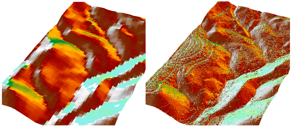
Figure 16.
DTM (left) and LiDAR Digital Surface Model (DSM) (right) databases showing the same area—20 years apart.
Figure 16.
DTM (left) and LiDAR Digital Surface Model (DSM) (right) databases showing the same area—20 years apart.

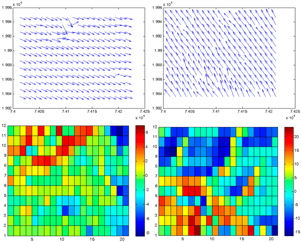
Figure 17.
Change detection analysis: results received by using the proposed mechanism of hierarchical registration and matching (left), and results received via the straightforward coordinate-based comparison (right). Values are in meters.
Figure 17.
Change detection analysis: results received by using the proposed mechanism of hierarchical registration and matching (left), and results received via the straightforward coordinate-based comparison (right). Values are in meters.

Figure 18 emphasizes the importance of working in a spatial hierarchical domain, as opposed to a simplified direct coordinate-based superposition. The three images describe statistical estimators calculated during the proposed hierarchical modeling. The top image shows the number of point-couplings that participated in the ICP matching for each frame (the higher the value, the better the correspondence); the middle image shows the SD of height value difference derived for both corresponding (matched) local frame surfaces after matching; and the bottom image shows the average height value difference derived for both corresponding local frame surfaces after matching (last two: the smaller the value, the better the correspondence). These three estimators provide some knowledge, or verification, of the reliability and stability of each local matching process. It is clear that there is high correlation among all three, again pointing to areas with less spatial correspondence, which mostly correspond to the areas identified in Figure 17. Overall, these results show the significance of the proposed modeling methodology and its capability to identify localized landform alterations in the terrain, as opposed to other commonly used techniques.
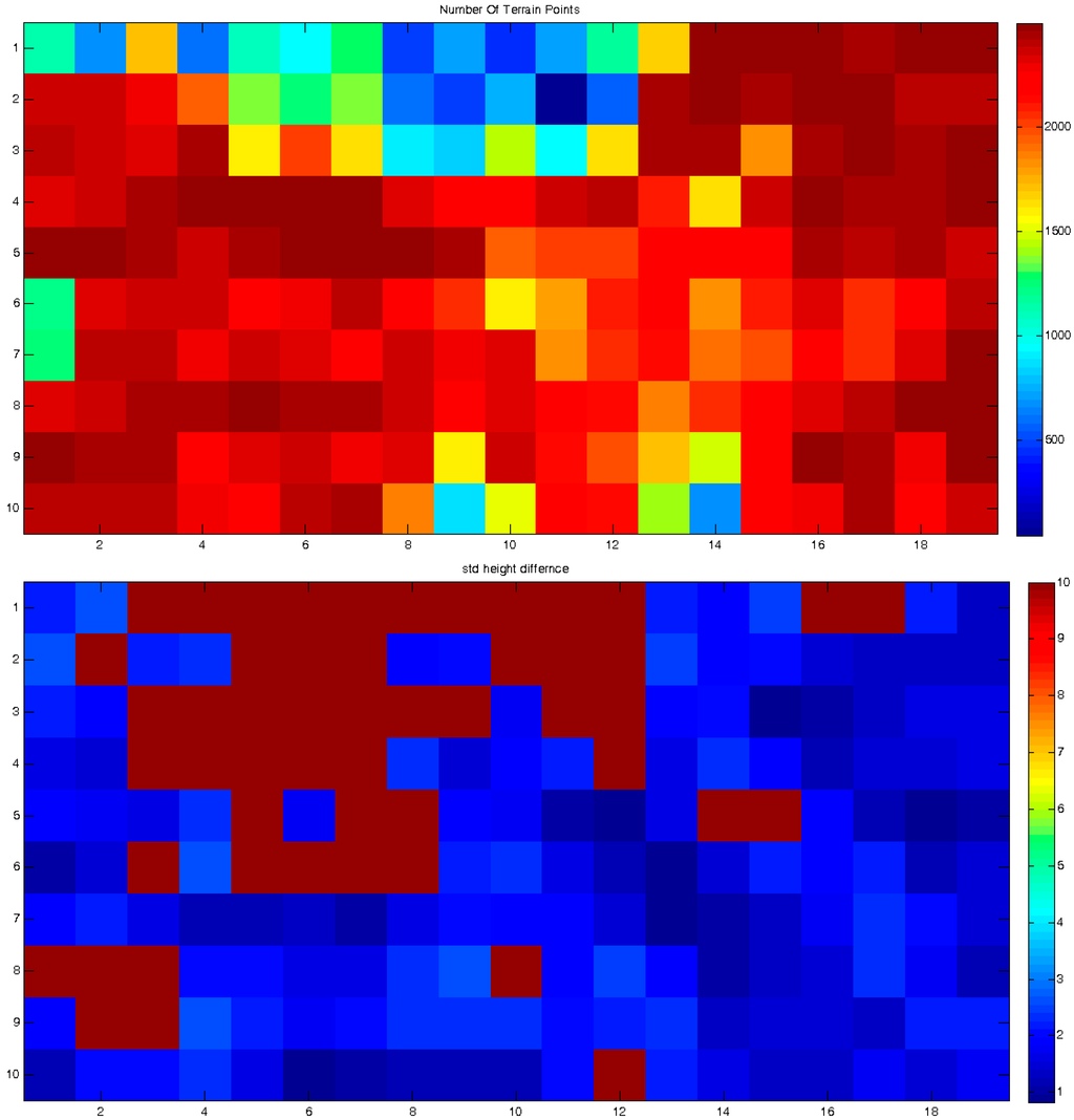
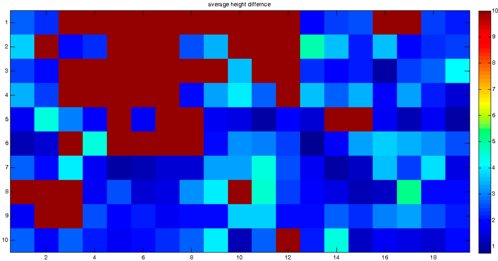
Figure 18.
Change detection analysis: statistical estimators reflecting on ICP process reliability; number of point-coupling (top), Standard Deviation (SD) of height value difference (middle) and average height value difference (bottom). Last two values are in meters.
Figure 18.
Change detection analysis: statistical estimators reflecting on ICP process reliability; number of point-coupling (top), Standard Deviation (SD) of height value difference (middle) and average height value difference (bottom). Last two values are in meters.


5. Discussion and Conclusions
The implementation of a hierarchical methodology for topographic and morphologic modeling of terrain surface representations was presented. This includes the development of an original algorithm for identifying the topographic skeletal structure, the implementation of a robust ranking registration process and an improved constrained-ICP matching algorithm. Together, such developments enable the monitoring and quantification of the geometric and spatial artifacts and discrepancies that exist when different terrain surfaces from different times are compared. This comprehensive framework enables proper definition, modeling and monitoring of the completely different databases’ spatial local interrelations, which by nature exist of varied-scale discrepancies. This ‘from global to local’ process validates that the mutual modeling is able to quantify both global and local spatial relations, as well as irregularities, thus preserving the topology, geometry and morphology of features (i.e., terrain relief characteristics) existing in the series of the terrain databases.
This novel hierarchical co-modeling enables the implementation of a comparison (change-detection) process for a given series of topographic databases, each acquired at a different time. By implementing statistical analyses on the monitored incongruity and discrepancy values, an automatic and precise definition of a land-region suspected of experiencing morphologic alteration is achieved. Also, the magnitude and trend of the alterations are identified and quantified with higher certainty. This is vital in order to preserve the spatially varying quality and trends that exist in the different databases and hence, as in the case of a change-detection process, achieves a uniform and seamless monitoring-data infrastructure. Analyses of change detection based on a series of topographic databases from various sources was presented, showing qualitative and reliable monitoring capabilities on a global scale, but also on a more localized one, thus, presenting more complex geomorphodynamic analysis capabilities, such as the calculation of velocity and acceleration attributes. These can be investigated not only within a global framework, but also locally, thanks to the quantification of localized monitoring that the hierarchical procedure encompasses. The presented modeling can be implemented on any number and combination of DTM databases, independently based on their data-structure, resolution and accuracy. This facilitates the kind of reliable and precise landform monitoring and warning infrastructure for geomorphodynamic analyses that is required for natural phenomena, such as landslides and earthquakes, as well as artificial changes.
Acknowledgments
This research work was supported by research fund number 2019466, Technion Security Research Foundation. Publication of this research work was supported by research fund 2019529, New-York/Metropolin Research Foundation.
Conflict of Interest
The author declares no conflict of interest.
References
- Beulter, G.; Mueller, I.; Neilan, R.E. The International GPS Service for Geodynamics (IGS): Development and Start of Official Service on 1 January 1994. Bull. Geod. 1994, 68, 39–70. [Google Scholar] [CrossRef]
- Kouba, J. Measuring Seismic Waves Induced by Large Earthquakes with GPS. Stud. Geophys. Geod. 2003, 47, 741–755. [Google Scholar] [CrossRef]
- Pe’eri, S.; Wdowinski, S.; Shtibelman, A.; Bechor, N.; Bock, Y.; Nikolaidis, R.; van Domselaar, M. Current plate motion across the Dead Sea Fault from three years of continuous GPS monitoring. Geophys. Red. Lett. 2002, 29. [Google Scholar] [CrossRef]
- Fejes, I.; Borza, T.; Busics, I.; Kenyeres, A. Realization of the Hungarian geodynamic GPS reference network. J. Geodyn. 1993, 18, 145–152. [Google Scholar] [CrossRef]
- Dalyot, S. The Footprint Network as a Solution to the Representation Problem in Monitoring Deformations. Bachelor’s Thesis, Israel Institute of Technology, Israel, 2000. [Google Scholar]
- Neilan, R.E. Position, Navigation and Timing: GPS Scientific Applications. Technical Paper; International GNSS Service Central Bureau: Jet Propulsion L aboratory, California Institution of Technology, Pasadena, CA, USA, 2008. [Google Scholar]
- Parry, R.B.; Perkins, C.R. World Mapping Today, 2nd ed.; Walter de Gruyter: Berlin, Germany, 2000. [Google Scholar]
- Kraus, K.; Karel, W.; Briese, C.; Mandlburger, G. Local Accuracy Measures for Digital Terrain Models. Photogramm. Rec. 2006, 21, 342–354. [Google Scholar] [CrossRef]
- ASTER GDEM Validation Team. ASTER Global DEM Validation: Summary Report. 2009. Available online: http://www.viewfinderpanoramas.org/GDEM/ASTER_GDEM_Validation_Summary_Report_-_FINAL_for_Posting_06-28-09[1].pdf (accessed on 15 February 2014).
- Rodriguez, E.; Morris, C.S.; Belz, J.E. A global assessment of the SRTM performance. Photogramm. Eng. Remote Sens. 2006, 72, 249–260. [Google Scholar] [CrossRef]
- Krieger, G.; Moreira, A.; Fiedler, H.; Hajnsek, I.; Werner, M.; Younis, M.; Zink, M. TanDEM-X: A Satellite Formation for High-Resolution SAR Interferometry. IEEE Trans. Geosci. Remote Sens. 2007, 45, 3317–3341. [Google Scholar] [CrossRef]
- Hrvatin, M.; Perko, D. Differences between 100-meter and 25-meter digital elevation models according to types of relief in Slovenia. Acta Geog. Slov. 2005, 45, 7–31. [Google Scholar] [CrossRef]
- Leigh, C.L.; Kidner, D.B.; Thomas, M.C. The Use of LiDAR in Digital Surface Modelling: Issues and Errors. Trans. GIS 2009, 13, 345–361. [Google Scholar] [CrossRef]
- Wilson, J.P.; Repetto, P.L.; Snyder, R.D. Effect of Data Source, Grid Resolution, and Flow-Routing Method on Computed Topographic Attributes, in Terrain Analysis: Principles and Applications; Wilson, J.P., Gallant, J.C., Eds.; John Wiley and Sons, Inc.: New York, NY, USA, 2000; Chapter 5. [Google Scholar]
- Dalyot, S.; Keinan, E.; Doytsher, Y. Landslide Morphology Analysis Model Based on LiDAR and Topographic Dataset Comparison. Surv. Land Inf. Sci. 2008, 68, 155–170. [Google Scholar]
- Avouac, J.P.; Ayoub, F.; Leprince, S.; Konca, O.; Helmberger, D.V. The 2005, Mw 7.6 Kashmir earthquake: Sub-pixel correlation of ASTER images and seismic waveform analysis. Earth Planet. Sci. Lett. 2006, 249, 514–528. [Google Scholar] [CrossRef]
- Feldmar, J.; Ayache, N. Rigid, Affine and Locally Affine Registration of Free-Form Surfaces. Int. J. Comput. Vis. 1996, 18, 99–120. [Google Scholar] [CrossRef]
- Frederiksen, P.; Grum, J.; Joergensen, L.T. Strategies for updating a national 3-D topographic database and related geoinformation. In Proceedings of the ISPRS XXth Congress, Istanbul, Turkey, 12–23 July 2004.
- Podobnikar, T. Production of integrated digital terrain model from multiple datasets of different quality. Int. J. Geogr. Inf. Sci. 2005, 19, 69–89. [Google Scholar] [CrossRef]
- Hahn, M.; Samadzadegan, F. Integration of DTMs using wavelets. Int. Arch. Photogram. Remote Sens. 1999, 32. Part 7-4-3 W6. [Google Scholar]
- Katzil, Y.; Doytsher, Y. Spatial rubber sheeting of DTMs. In Proceedings of the 6th Geomatic Week Conference, Barcelona, Spain, 8–11 February 2005.
- Rusinkiewicz, S.; Levoy, M. Efficient variants of the ICP algorithm. In Proceedings of the 3D Digital Imaging and Modeling, Quebec City, Canada, 28 May–01 June 2001; pp. 145–152.
- Zhengyou, Z. Iterative point matching for registration of free-form curves and surfaces. Int. J. Comput. Vis. 1993, 13, 119–152. [Google Scholar] [CrossRef]
- Huttenlocher, D.P.; Klanderman, G.A.; Rucklidge, W.J. Comparing images using the Hausdorff distance. IEEE Trans. Pattern Intell. Mach. Intell. 1993, 9, 850–863. [Google Scholar] [CrossRef]
- Siriba, D.; Dalyot, S. Automatic Georeferencing of Non-Geospatially References Provisional Cadastral Maps. Surv. Rev. 2012, 44, 142–152. [Google Scholar] [CrossRef]
- Mount, D.M.; Netanyahu, N.S.; Le Moigne, J. Efficient Algorithms for Robust Feature Matching. Pattern Recognit. 1998, 32, 17–28. [Google Scholar] [CrossRef]
- Besl, P.J.; McKay, N.D. A method for registration of 3-D Shapes. IEEE Trans. Pattern Anal. Mach. Intell. 1992, 14, 239–256. [Google Scholar] [CrossRef]
- Gruen, A. Least squares matching: A fundamental measurement algorithm. In Close Range Photogrammetry and Machine Vision; Atkinson, K.B., Ed.; Whittles Publishing: Caithness, UK, 1996; Chapter 8. [Google Scholar]
- Eggert, D.; Dalyot, S. Octree-Based SIMD Strategy for ICP Registration and Alignment of 3D point clouds. ISPRS Ann. Photogramm. Remote Sens. Spat. Inf. Sci. 2012, 3, 105–110. [Google Scholar] [CrossRef]
- Jenson, S.K.; Dominique, J.O. Extracting topographic structure from digital elevation data for geographic information system analysis. Photogramm. Eng. Remote Sens. 1988, 54, 1593–1600. [Google Scholar]
- Keisler, H.J. Elementary Calculus: An Infinitesimal Approach; Prindle, Weber & Schmidt: Boston, MA, USA, 1986. [Google Scholar]
- Varady, T.; Hermann, T. Best Fit Surface Curvature at Vertices of Topologically Irregular Curve Networks. In Proceedings of the 6th IMA Conference on the Mathematics of Surfaces, Brunel University, England, UK, September 1994; pp. 411–427.
- Goshtasby, A.A. 2-D and 3-D Image Registration for Medical, Remote Sensing, and Industrial Applications; Wiley Press: Hoboken, NJ, USA, 2005. [Google Scholar]
- Baker, R. A Second Look at Taylor’s Stability Chart. J. Geotech. Geoenviron. Eng. 2003, 129, 1102–1108. [Google Scholar] [CrossRef]
© 2015 by the authors; licensee MDPI, Basel, Switzerland. This article is an open access article distributed under the terms and conditions of the Creative Commons Attribution license (http://creativecommons.org/licenses/by/4.0/).