Abstract
Shallow landslides are one of the most common natural hazards in Brazil and worldwide. Susceptibility maps are powerful tools to analyze the spatial probability of shallow landslide occurrences. The outputs of susceptibility maps strongly depend on the type of landslide inventory used. The aim of this study is to examine the influence of different inventories on shallow landslide susceptibility modeling using the different methods LR, SVM, and XGBoost. Three different shallow landslide inventories were compiled following a single extreme rainfall event in the Ribeira Valley, São Paulo, Brazil. The results indicate that inventories generated through different landslide detection methods and imagery produce diverse susceptibility maps, as evidenced by the calculated Cohen’s Kappa coefficient values (0.33–0.79). The agreement among the models varied depending on the specific model: LR exhibited the highest agreement (0.79), whereas SVM (0.36) and XGBoost (0.33) showed lower numbers. Conversely, the accuracy numbers suggest that XGBoost achieved the highest success rate in terms of AUC (85–78%), followed by SVM (82–76%), and LR (80–71%). Inventories obtained through different detection methods, using distinct datasets, can directly influence the susceptibility assessment, leading to varying classifications of the same area. These findings demonstrate the importance of well-established landslide mapping criteria.
1. Introduction
The impacts of climate change and the more frequent occurrence of extreme events underscore the significance of studying climate-related hazards, such as landslides. The increasing frequency of extreme rainfall events has resulted in fatalities and economic loss worldwide [1]. Susceptibility maps are a powerful tool to analyze the spatial probability of landslide occurrence [2]. Shallow landslide susceptibility maps (LSM) are constructed based on several conditioning factors and inventories of past landslide events [3,4]. Landslides often occur under similar geological, geomorphological, hydrogeological, and climatic conditions as observed in the past, which underscores the importance of considering these factors for generating LSMs [2]. The conditioning factors encompass various types of data, including digital elevation model (DEM) derived factors (e.g., elevation, slope degree, aspect, curvature), climatic factors (e.g., precipitation), factors derived from river networks (e.g., stream density, distance to rivers), geological factors (e.g., geology, lithology, distance to faults), soil property factors, and land cover factors [5]. The landslide inventory is a crucial dataset, both for training the models and validating the model results.
A large variety of methods can be used for landslide susceptibility mapping. They can be grouped and classified as multi-criteria methods [6,7,8], statistical methods [9,10,11], geotechnical engineering methods [12,13,14], and machine-learning (ML) methods [15,16,17,18]. ML and statistical approaches have become common to study landslides. Logistic regression (LR) is one example of a popular multivariate statistical model applied for creating LSMs worldwide [9,19,20,21,22,23]. ML tools are frequently used for landslide recognition [24,25] and susceptibility assessment [16,17]. ML is capable of managing large volumes of data and establishing complex interconnections between the input data [26]. Support vector machine (SVM) is a popular ML algorithm commonly used in landslide studies. SVM is a supervised-learning algorithm used for classification and regression tasks [26,27,28]. Extreme gradient boosting (XGBoost), another important algorithm, is an ensemble-learning method based on decision trees, specifically designed for gradient boosting [17,26,28]. ML methods are widely regarded as robust data-driven models, often achieving higher accuracy compared to other susceptibility methods [17]. However, this is not always the case, and the present study provides a critical examination, comparing susceptibility maps derived from various shallow landslide inventories and susceptibility assessment methods.
In the last years, an increasing number of studies have been dealing with the influence of errors and completeness of inventories in landslide susceptibility assessment [29,30,31,32,33]. Inventories can be constructed by a variety of methods (manual, semi-automatic, and automatic), being point or polygon-based, and can be classified as historical, event-based, seasonal, or multi-temporal [3]. Inventories constructed by different agents can influence the classification accuracy; the classification system used to define the types of landslides [34,35,36,37] together with visual mapping criteria are also important aspects to consider in landslide susceptibility assessment [38]. Ensuring a precise location of landslide polygons or points in inventories is consistently emphasized as essential for generating dependable susceptibility maps [3,29,30,39,40].
Data-driven models rely on the quality of input data, and different inventories from various sources influence the outcomes [31]. The study site has an important role in the susceptibility to landslides, since the heterogeneity of the local geomorphology and geology impacts the analysis. Environments with low diversity are less affected by less accurate inventories than more diverse and complex environments [32]. However, the extent of this influence varies depending on the study site and the quality of the inventory; thus, using accurate inventories is always preferable.
Rainfall-induced landslides are common in Brazil in the summer season (December to March) due to the occurrences of thunderstorms. Several high-magnitude events occurred in the last years resulting in social and economic damages: São Sebastião (2023), Petrópolis (2022), Guarujá (2020), Itaóca (2014), Rio de Janeiro mountain region (2011). Between 1988 and 2022, 4146 deaths caused by landslides were registered in Brazil, an average of 118 fatalities per year [41]. In Brazil, the primary entity responsible for financing risk reduction is the federal government. However, the budget allocated to this sector has decreased over the past decade. In 2021, the investment budget was 66% lower than it was in 2013 [42]. The high number of deaths is directly linked to the lack of governmental strategic policies for territorial management aimed at addressing disasters. Out of every 100 inhabitants, nine reside in locations vulnerable to disasters [43]. Climate change has introduced numerous challenges globally. In Latin America, these challenges are compounded by a historical legacy of socio-economic inequalities and environmental degradation, shaped by its colonial past [42,44]. Therefore, given the significant socio-economic impact of landslides in Brazil, it is crucial to investigate and assess the application of manual and semi-automatic methods for constructing landslide inventories and their influence in susceptibility assessment using different ML and statistical approaches. Thus, the aim of this study is to examine the influence of different inventories on shallow landslide susceptibility modeling using different methods (LR, SVM, and XGBoost) in Brazil. Different inventory acquisition methods and datasets can directly impact susceptibility assessment, resulting in diverse classifications of an area.
2. Study Area
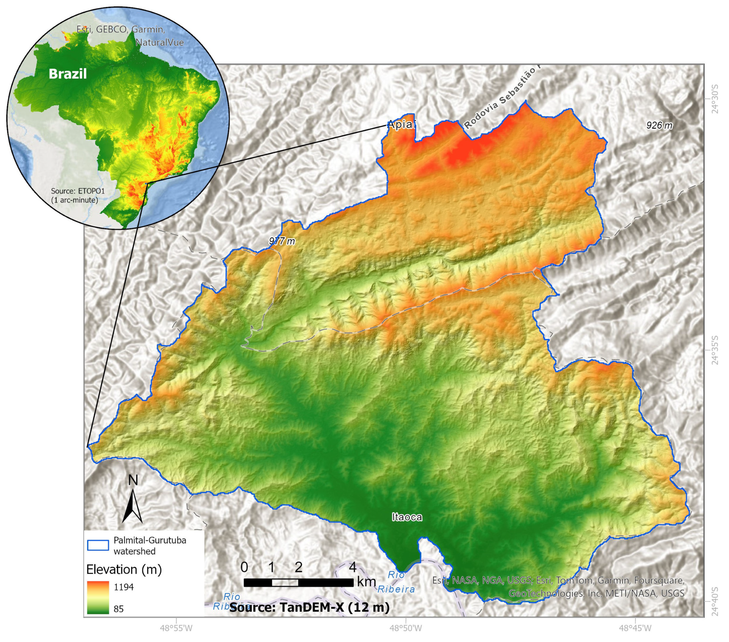
The Palmital–Gurutuba watershed (221 km2) is located between the Apiaí and Itaóca municipalities in the state of São Paulo, southeastern Brazil (Figure 1). Both municipalities are predominantly rural areas. Apiaí has 25,200 inhabitants and a total area of 974 km2, and Itaóca 3200 inhabitants in a total area of 183 km2 [45]. The Palmital–Gurutuba watershed is part of hydrographic unit 11 in São Paulo state, known as Ribeira do Iguape e Litoral Sul. The study area is characterized by steep slopes and elevations ranging from 85 to 1194 m above sea level (m.a.s.l.), and it is covered by the Atlantic Forest. The geology consists of Archean–Proterozoic igneous and metamorphic rocks, with a predominance of granite [46,47]. The soil types present in the area include cambisols, leptosols, acrisols, and gleysols [48]. The climate is classified as Cfa (humid subtropical climate) according to Köppen’s classification [49], with temperatures ranging from 11–30 °C [50].

Figure 1.
Location and topography of the study area.
On 12 January 2014, a period of heavy precipitation triggered numerous mass movements in the area. The region exhibits a medium to high susceptibility to debris flows, which are predominantly triggered by shallow landslides in Brazil [51]. In Itaóca, occurrences of shallow landslides and debris flows were triggered in close proximity to the city center, causing significant erosion of riverbanks and the displacement of large boulders and logs [52]. Consequently, Itaóca emerged as the area most severely impacted by landslides [53].
3. Materials and Methods
3.1. Shallow Landslide Inventories
Three different polygon-based inventories were used to produce shallow landslide susceptibility maps (Figure 2). These inventories pertain to the landslide event that occurred on 12 January 2014, in Itaóca and Apiaí. For all three inventories, certain criteria were adopted to identify shallow landslides through image interpretation. These criteria include the absence of vegetation, drainage network distance, altimetric variation, planar rupture surface, slope position, shape, and size [33].

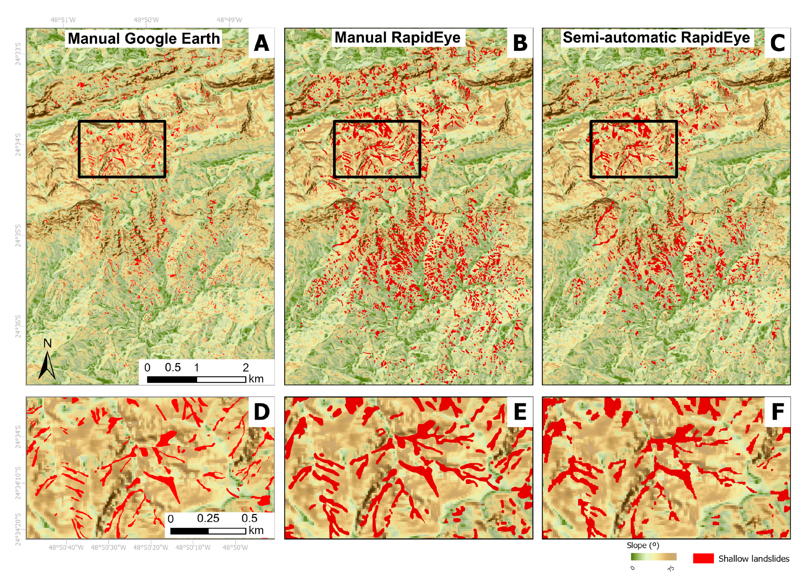
Figure 2.
Inventories used as input to produce shallow landslide susceptibility maps: (A) manual—Google Earth images; (B) manual—RapidEye satellite image; (C) semiautomatic—RapidEye satellite image; (D) zoom of A; (E) zoom of B; and (F) zoom of C.
The first inventory (INV1) was manually created using freely accessible images from Google Earth Pro (Figure 2A,D). The most recent images available for the study area were satellite images from SPOT 5 (with a spatial resolution of 2.5 m) dated 8 October 2014, which were captured nine months after the landslide event [33]. The second inventory (INV2) was manually constructed using a RapidEye satellite image (5 m spatial resolution) dated 30 January 2014, captured eighteen days after the event, with five spectral bands (blue, red, green, red edge, and near-infrared (NIR)) [54] (Figure 2B,E). The third inventory (INV3) was semi-automatically constructed using the same RapidEye image as for INV2 [25]. An object-based image analysis approach (OBIA) was applied, using spatial, spectral, and morphological metrics for the detection and classification of shallow landslides. As it is common with image classification techniques, results included false positive errors. After a visual and manual verification, these errors were excluded, and only the shallow landslides correctly identified by the approach were considered.
3.2. Thematic Variables
A total of seven thematic variables were used (Figure 3), according to their influence on shallow landslide susceptibility [4,38]. Five variables representing morphological and hydrological parameters commonly used in susceptibility studies in Brazil (aspect, plan curvature, elevation, slope, and flow accumulation) [38] were extracted from a 12 m resolution DEM (TanDEM-X—License number: DEM-HYDR3714), predating the landslide event. Thus, each final susceptibility map was based on a resolution of 12 m. The lithology map of the Palmital–Gurutuba watershed (scale 1:100,000) incorporated data from geological maps created by Faleiros et al. [46] and the soil map (scale 1:250,000) was created by Rossi [48]. These are the best data available for the study area.
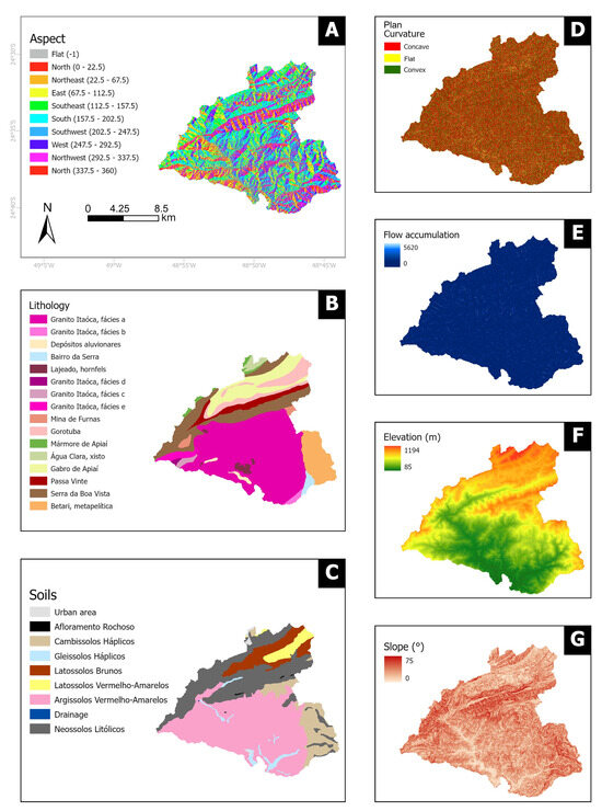
Figure 3.
Thematic variables: (A) aspect; (B) lithology; (C) soil; (D) plan curvature; (E) flow accumulation; (F) elevation; and (G) slope.
3.3. Susceptibility Assessment and Models
All inventories were randomly split, resulting in two pair sets of testing (30%) and training (70%) samples. The models required the same proportion of landslide and non-landslide samples in training and validation sets. The inventories were constructed based on three different methods and datasets, which is the reason why the total number of shallow landslides varied (Table 1). Three different susceptibility models were applied: LR, SVM, and XGBoost [55]. The final maps were classified into five classes using quantile breaks: very low, low, moderate, high, and very high. Each susceptibility class contains an equal number of pixels. The equal distribution of pixels across susceptibility classes was chosen to facilitate comparison of how different landslide inventories influence model performance. The analysis was performed using ArcGIS Pro 3.1.2 and R 3.6.3 software.

Table 1.
Inventory types, total number or landslide polygons, and number of samples.
3.3.1. Logistic Regression (LR)
LR is one of the most commonly applied statistical methods worldwide for landslide susceptibility [4,19]. However, only a few studies have applied it in Brazil [9,20,23]. LR is a multivariate model used to effectively analyze the relationship between dependent and independent variables in landslide occurrence. The dependent variable is categorical (e.g., presence or absence), while the independent (explanatory) variables can be categorical, numerical, or a combination of both [19,56,57]. In this study, the dependent variable represents landslide occurrence, with a value of 1 indicating a landslide and 0 indicating non-landslides. The expression for the dependent variable is presented in Equation (1) and the expression for the probability of occurrence, P, in Equation (2).
3.3.2. Support Vector Machine (SVM)
SVM is a supervised machine-learning algorithm proposed by Vapnik [58] based on statistical-learning theory. SVM is widely applied for landslide susceptibility mapping [26,28,57], but it has not been extensively used in Brazil [38]. This algorithm aims to generate a decision surface that separates two classes, such as landslide and non-landslide [28]. The SVM algorithm relies on two main principles: the optimal classification hyperplane and the use of a kernel function [27]. The classification function is presented in Equation (3).
where x represents the input variables, y represents the output or target vector (with values of 1 and 0), is the Lagrange multiplier, b is the offset from the origin of the decision surface, and K represents the kernel function [28].
The SVM model was configured with the radial basis function (RBF) kernel, which is suitable for capturing non-linear relationships between landslide occurrence and conditioning factors. The model was regularized using the C parameter, set to 1.0, controlling the classification error, and the parameter, set to 0.3, balancing the influence of individual data points.
3.3.3. Extreme Gradient Boosting (XGBoost)
XGBoost is based on the gradient boosting principle, incorporating a number of boosting iterations (n), column samples, and subsamples [26]. It is a powerful supervised ensemble ML approach that integrates multiple decision tree models to generate a classification with higher accuracy through an iterative process [17]. XGBoost combines several classification and regression tree models using gradient boosting to achieve better model precision. It aims to minimize the objective function, which is the sum of the loss function and a regularization term, to control overfitting [28]. The classification function is presented in Equation (4).
where represents the expected value of the th model for the sample i, denotes the newly added tth model, refers to the regularization term, C is a constant, and the outermost represents the error [17].
The XGBoost model was configured with a total of 50 iterations, meaning the model was trained with 50 trees, and 60% of the training data was used at each iteration, which helps reduce overfitting. Additionally, 75% of the available features were used for constructing each tree, which also aids in preventing overfitting. Regarding the tree depth, the model used the default setting 6, which is a common choice as it strikes a balance between underfitting and overfitting.
XGBoost has been widely applied for landslide susceptibility mapping [17,26,28,59] but it has been not applied in Brazil [38].
3.4. Evaluation of Spatial Agreement
The evaluation of agreement among models derived from different inventories was conducted using Cohen’s Kappa index [60], a method previously applied in comparing landslide susceptibility models [9,30]. Cohen’s Kappa, denoted as k, is expressed in the following Equation (5).
In this equation, represents the probability of observed agreement between two rasters, while represents the hypothetical probability of chance agreement. A value of k 0 indicates no relationship between the models, while a value of 1 implies complete agreement. Cohen’s Kappa was calculated using the r.kappa tool in QGIS.
3.5. Accuracy Assessment
The accuracy assessment of the scenarios was performed using success and prediction rate curves. They enable the comparison between shallow landslide susceptibility scenarios by relating testing sets and the area defined as susceptible. These curves are commonly used for validating landslide susceptibility models [9,11,61,62]. The assessment is based on calculating the area under the success rate curve and prediction rate curve (AUC). A larger AUC indicates better performance of the scenario in terms of accuracy.
4. Results
4.1. Comparison of the Inventory Characteristics
The three inventories used were constructed based on different datasets and by different methods. As a result, they do not have the same values (Table 2). INV1 has the smallest values, except for the total number of polygons. INV2 has the largest total area identified, and INV3 presents the lowest number of polygons. INV3 recognized 27% fewer landslides than INV2, and the average and minimum areas are similar to INV2.
Table 2.
Shallow landslide polygon characteristics.
4.2. Shallow Landslide Susceptibility and Model Accuracy
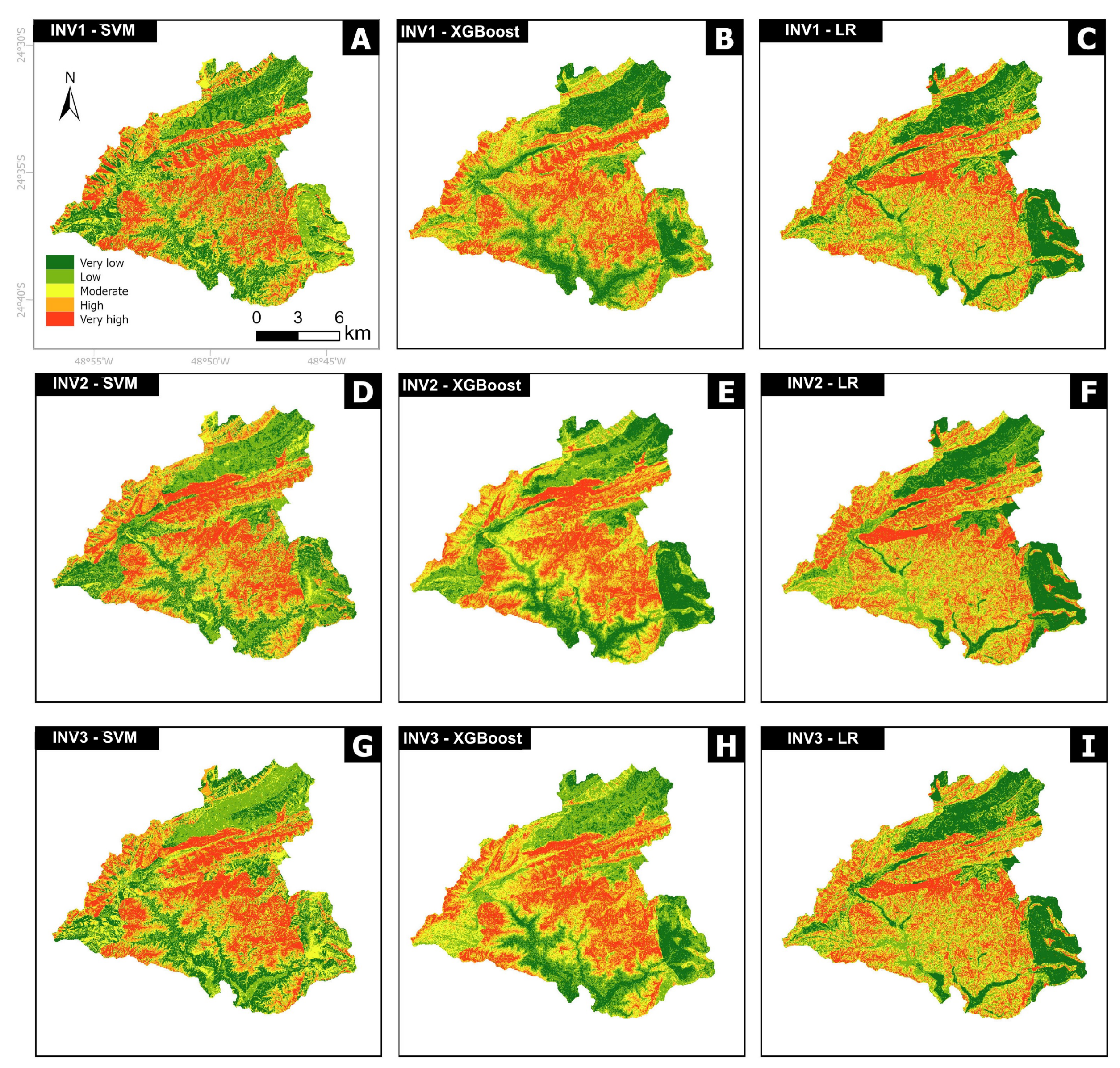
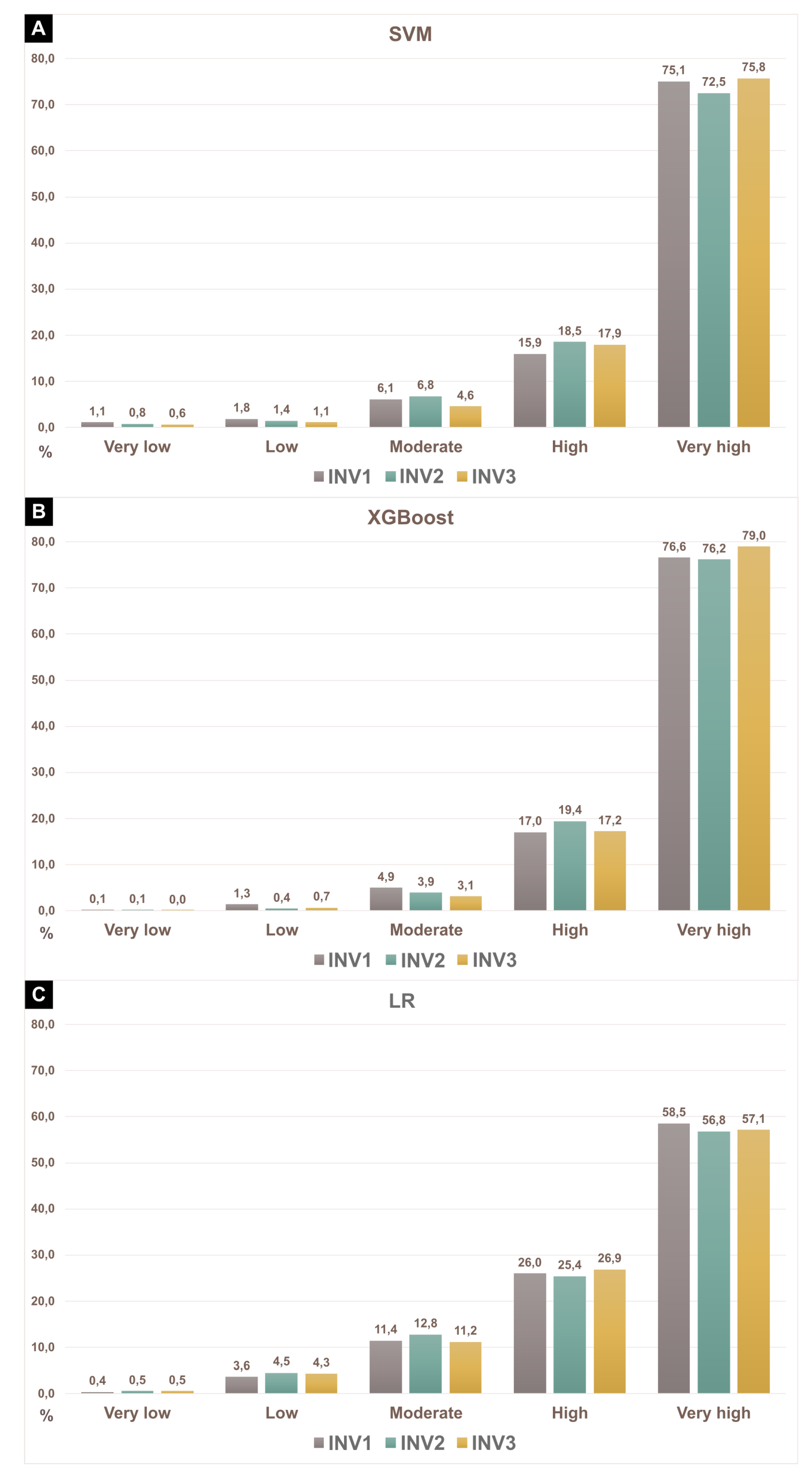
Nine susceptibility scenarios were defined (Figure 4). Upon visually examining the maps, discernible differences in the spatial distribution of susceptibility emerged resulting from the different input inventories. The comparison of accuracy values, as represented by AUC (success and prediction), across all training and test sets revealed variations dependent on the chosen input inventory and model type (Table 3). For LR, the mean values ranged from 0.75 to 0.77 for training sets and from 0.71 to 0.80 for test sets. In the case of SVM, mean values spanned from 0.86 to 0.88 for training sets and from 0.76 to 0.82 for test sets. XGBoost exhibited mean values within the range of 0.91 to 0.94 for training sets and 0.78 to 0.85 for test sets. LR exhibits lower accuracy rates when compared to SVM and XGBoost. Figure 5 illustrates the occurrence of shallow landslide scars in each susceptibility class for SVM, XGBoost, and LR models. The “very high” susceptibility class concentrates the majority of landslides in all models and inventories, indicating a similar performance across all scenarios for this class. However, LR exhibits a more dispersed distribution among “low”, “moderate”, and “high” classes. This may elucidate the lower accuracy rates observed in LR scenarios. The dispersed distribution of shallow landslide scars among susceptibility classes in the logistic regression-based LSMs indicates that the model may have difficulty accurately distinguishing between different levels of landslide susceptibility. A more dispersed distribution of shallow landslide scars among susceptibility classes can lead to decreased accuracy, because it indicates that the model’s predictions are less certain and may not align well with the true susceptibility levels observed in the data. In contrast, if the SVM and XGBoost models provide a more concentrated distribution of shallow landslide scars among susceptibility classes, it suggests that the model’s predictions are more confident and likely to be closer to the true susceptibility levels.

Figure 4.
Susceptibility maps constructed based on three algorithms: (A) INV1 SVM; (B) INV1 XGBoost; (C) INV1 LR; (D) INV2 SVM; (E) INV2 XGBoost; (F) INV2 LR; (G) INV3 SVM; (H) INV3 XGBoost; and (I) INV3 LR.
Table 3.
Success and prediction rates for each susceptibility map constructed based on LR, SVM, and XGBoost for each inventory.
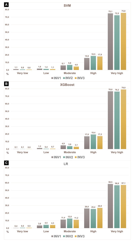
Figure 5.
Presence of shallow landslide scars in each susceptibility class for different input inventories and models: (A) SVM; (B) XGBoost; and (C) LR.
Across all three models, INV1 consistently exhibited lower prediction accuracy rates when compared to INV2 and INV3. These results provide evidence that the performance of all models increases significantly when an inventory based on imagery a few days after the event is used. The variation in prediction rates among the input inventories amounted to 9.5%, 6.7%, and 5.6% for LR, XGBoost, and SVM, respectively. Meanwhile, the variation in prediction rates among the models amounted to 7.1%, 5.3%, and 4.3% for INV1, INV2, and INV3. These findings confirm that models are more sensitive to changes in input inventories than to changes in the model itself.
4.3. Spatial Comparison Between Susceptibility Maps of Palmital–Gurutuba Watershed
The Cohen’s Kappa index (k) was employed to evaluate the level of agreement among the susceptibility maps of the Palmital–Gurutuba watershed derived from different input inventories and ML algorithms. Consequently, the k value for each pair of shallow landslide inventories was calculated for each algorithm (Table 4).
Table 4.
The Cohen’s Kappa indexes (k) derived from the comparison between the shallow landslide inventories and the models. The k index for each susceptibility class—very low (VL), low (L), moderate (M), high (H), and very high (VH)—is separately indicated.
From Table 4, it can be seen that the LSMs showed an overall mean k value of 0.5; this constitutes a moderate level of agreement. Regarding the LR algorithm, the k values ranged from 0.66 to 0.80 (mean 0.73), indicating that a substantial level of agreement was observed among these inventories. For the SVM and XGBoost algorithms, the k values range from 0.36 to 0.47 (mean 0.41) and 0.34 to 0.42 (mean 0.37), respectively, indicating a fair to moderate degree of agreement. A high spatial agreement was observed between the susceptibility maps produced by the LR algorithm, indicating that this algorithm is less sensitive to changes in the input inventory than SVM and XGBoost. Table 4 additionally illustrates the degree of agreement for each susceptibility class. The “very high” class exhibits the highest k values across all models, followed by the “very low” class. This suggests that, despite variations between susceptibility maps constructed using different input inventories, there is a similarity between the highest and lowest susceptibility classes.
5. Discussion
The influence of landslide inventories in the construction of landslide susceptibility maps has been analyzed worldwide in recent years [29,30,31,32,33,63]. In this study, we examined potential variations in LSMs generated for the same study site by employing different input inventories. Specifically, our focus was on assessing differences in accuracy rates and the distribution of susceptibility classes across the Palmital–Gurutuba watershed.
The three inventories used showed significant differences, such as the total number of polygons and total area (Table 2). The differences in the number of polygons and area can be explained by various reasons. Despite the expert knowledge used in the manual mapping, INV1 shows the lowest numbers (e.g., total area, average area), with the exception of the total number of polygons. This difference from the other inventories can be attributed to the higher resolution of the satellite images and the acquisition date of the images used, which were acquired eight months after the event and represent the most recent data available in Google Earth. During this time, vegetation growth covered the landslides, making it increasingly challenging to identify them [64,65]. Additionally, the landslide scars underwent processes of instability and became susceptible to erosive processes [66], which further complicated their delineation [67]. Despite the absence of regularly updated data, Google Earth offers substantial advantages that significantly enhance its value as a visualization tool. The platform provides easily accessible high-resolution imagery, and its user-friendly interface contributes to its utility for data collection, exploration, and validation [68]. INV2 shows the largest total area, which is influenced by using the closest satellite image available to the event acquired only two weeks after the event and the expert knowledge used in the manual mapping. INV3 shows the lowest number of polygons. By applying an object-based approach, it was possible to create landslides polygons comparable in size and number as created by manual mapping. However, according to Dias et al. [25], some small shallow landslides were missed by OBIA and some neighboring landslides were incorrectly merged into larger polygons, resulting in the largest maximum area and the smallest number of polygons.
According to the comparative AUC performance evaluation, there is a difference between the training and testing metrics for scenarios using INV1. This can be attributed to the fact that it was built using an inventory that is not considered the most reliable. INV1, which was manually generated from Google Earth images, may not have captured the full extent of the landslides or accurately reflected the spatial distribution of the event being modeled. This could lead to a less accurate representation of the conditions in the test set, explaining the discrepancy in performance. It is important to highlight that the quality of the data, especially the inventory used, plays a crucial role in the model’s ability to generalize well to unseen data. Thus, the observed difference between training and test results might be more closely related to the limitations of the inventory rather than overfitting.
XGBoost is identified as more efficient in the construction of LSMs compared to other methods. The second and third best models are SVM and LR, respectively, a pattern consistent with the findings reported by Pyakurel et al. [26]. It is noteworthy to emphasize the consistent similarity in the results between INV2 and INV3 across all methods. Despite the differences, INV2 and INV3 show significant similarities, demonstrating certain advantages of semi-automatic object-based mapping over manual mapping, which is considered a time-consuming and subjective procedure [3,39,69]. This underscores the suitability of semi-automatically created inventories for application in predictive models. The study by Pyakurel et al. [26] compared the performance of five supervised models (LR, Random Forest, XGBoost, SVM, and extremely randomized trees classifier) to predict earthquake-induced landslide susceptibility in Nepal, and LR exhibited the lowest accuracy rates (74%), consistent with our results. Similar accuracy rates between 0.7 and 0.8 for LR were also reported in other landslide susceptibility studies [9,22]. Sahrane et al. [32] analyzed the impact of landslide inventory completeness and concluded that the accuracy of LSMs can be influenced by the loss of information in inventories. In our study, INV1 exhibited lower accuracy rates across all models due to the loss of original shape information of landslides soon after the event. Inventory completeness is a crucial aspect when comparing them. INV2 is regarded as the most accurate inventory in our study, while INV1 and INV3 encounter some completeness issues, with the former attributed to the utilization of less-than-ideal imagery eight months after the event, and the latter attributed due to errors, such as delineation of scars, committed by the OBIA approach. Another relevant finding is the good performance of INV3. The semi-automatic object-based inventory exhibited the best prediction rates in all models, with the numbers being very close to those achieved by INV2, which is considered the most accurate inventory. This highlights two important points: firstly, the suitability of semi-automatic inventories in susceptibility analysis is a positive development, and secondly, it raises concerns about the good performance (in this case, the best one) of an inventory that lacks 38% completeness. None of the inventories had a prediction rate lower than 70%, indicating that all nine scenarios constructed performed well, although some performed better than others. The influence of the input inventory is also a subject of discussion in studies conducted by Bordoni et al. [30] and Dias and Grohmann [33]. Both studies assert that when inventories are associated with the same rainfall event but developed with different criteria, the susceptibility distribution is affected by the choices made.
A noticeable variation was identified in the final LSMs when employing different input inventories and models (Figure 4). The results from the k coefficient analysis indicate that the distribution of landslide susceptibility classes, derived from various input inventories, exhibits spatial variations. Despite the models showing some spatial discrepancies, substantial or moderate spatial agreement was observed in most comparisons, especially in areas with very high susceptibility. According to our findings, LR demonstrated a more consistent spatial agreement with all input inventories, suggesting that it is less sensitive to changes. However, SVM and XGBoost models displayed spatial variations in areas with “low”, “moderate”, and “high” susceptibility, indicating that they are more sensitive to changes. These variations may stem from the complexity of each model and the characteristics of the input inventory. Therefore, it is not reasonable to anticipate identical LSMs, even when their accuracy rates are similar. Comparable findings were reported by Barella et al. [9] in Minas Gerais, Brazil, using statistical models, and by Bordoni et al. [30] in Italy using a data-driven method. Barella et al. [9] also underscore the importance of employing polygon-based inventories instead of point-based inventories, as the former produce more consistent maps due to a higher number of pixels with similar properties within a landslide polygon.
When comparing the input inventories INV1, INV2, and INV3, as well as the models LR, SVM, and XGBoost based on the accuracy assessment (Table 3) and spatial agreement (Table 4), it can be observed that using INV1, an inventory affected by a loss of information regarding the original shape of the landslide scars, decreased the prediction accuracy by almost 10% using LR, and 6.7% and 5.6% using XGBoost and SVM, respectively. The difference can reach almost 14% when comparing the worst scenario (INV1-LR) and the best one (INV3-XGBoost). In all models, the spatial agreement (k) between INV2 and INV3 consistently demonstrates higher values than between INV1 and INV2, and INV1 and INV3. These results confirm that the input inventory has a more pronounced impact on the accuracy rate variation than altering the model classifiers in assessing landslide susceptibility. Nevertheless, both the input inventory and the chosen model/algorithm introduce variations in the final susceptibility maps, emphasizing the importance of providing detailed descriptions of the input data and analysis in landslide studies.
6. Conclusions
The influence of different input shallow landslide inventories on susceptibility estimation was assessed using three distinct inventories and models in the Gurutuba–Palmital watershed in Brazil. It is crucial to emphasize that the results obtained pertain to pixel-based models employing both manual and semi-automatic inventories in a tropical environment. The final LSMs constructed using INV1, INV2, and INV3 exhibit similar and robust predictive capabilities (71% to 85%). Inventories obtained through different detection methods, using different datasets related to the same rainfall event, can directly influence the susceptibility assessment, leading to varying classifications of an area based on the presence of shallow landslides.
INV1 demonstrated that using an image acquired eight months after the event resulted in less accurate maps, highlighting the importance of an accurate inventory as a variable in the models. An inventory generated through visual interpretation and established criteria (INV2), alongside a semiautomatic inventory created using OBIA (INV3), both employing the same high-resolution satellite images, yielded similar accuracy and spatial agreement. This outcome demonstrates the suitability of semi-automatic methods for shallow landslide susceptibility assessment in tropical environments such as Brazil.
The spatial agreement between the maps and the distribution of susceptibility classes also varies depending on the inventory and the algorithm used. These findings underscore the significance of the input inventory type used in creating susceptibility maps, as it directly impacts the accuracy and reliability of the resulting maps. Hence, it is imperative to provide details regarding the criteria and dataset in compiling a shallow landslide inventory for susceptibility assessment. This information enables local stakeholders and decision makers to place trust in LSM derived from inventories that most faithfully reflect the hazards they aim to address, particularly when predictive accuracies of susceptibility models are comparable. In future investigations, further exploration into the influence of diverse landslide inventories could be pursued through alternative methodologies, including deep-learning techniques. Such endeavors would contribute to a deeper understanding of the complexities involved and potentially enhance the efficacy of landslide-susceptibility assessments.
Author Contributions
Conceptualization, H.C.D. and C.H.G.; methodology, H.C.D., D.H., and C.H.G.; software, H.C.D.; validation, H.C.D.; formal analysis, H.C.D.; resources, H.C.D., D.H., and C.H.G.; data curation, H.C.D., D.H., and C.H.G.; writing—original draft preparation, H.C.D.; writing—review and editing, H.C.D., D.H., and C.H.G.; visualization, H.C.D., D.H., and C.H.G.; supervision, D.H. and C.H.G.; project administration, C.H.G.; funding acquisition, H.C.D. and C.H.G. All authors have read and agreed to the published version of the manuscript.
Funding
The São Paulo Research Foundation (FAPESP) supported H.C.D. (No. 2019/17261-8, 2022/01534-8), and C.H.G. (No. 2019/26568-0, 2023/11197-1). D.H. was supported by the Austrian Research Promotion Agency (FFG) in the Austrian Space Applications Program (ASAP) through the project LEONA (No: FO999921058).
Institutional Review Board Statement
Not applicable.
Informed Consent Statement
Not applicable.
Data Availability Statement
Landslide inventory used in this study is available in Zenodo at https://doi.org/10.5281/zenodo.14173402 (accessed on 13 February 2025).
Acknowledgments
The authors gratefully acknowledge the São Paulo Research Foundation (FAPESP) and CAPES for providing financial support. Additionally, the Editor-in-Chief and the anonymous reviewers are acknowledged for their valuable criticism and suggestions, which have contributed to the enhancement of this paper.
Conflicts of Interest
The authors declare no conflicts of interest.
Abbreviations
The following abbreviations are used in this manuscript:
| AUC | Area under the curve |
| Cfa | Humid subtropical climate |
| DEM | Digital elevation Model |
| INV1 | First inventory |
| INV2 | Second inventory |
| INV3 | Third inventory |
| LSM | Landslide susceptibility maps |
| LR | Logistic regression |
| ML | Machine learning |
| NIR | Near-infrared |
| OBIA | Object-based image analysis |
| TanDEM-X | TerraSAR-X add-on for digital elevation measurement |
| SPOT 5 | Satellite Pour l’Observation de la Terre 5 |
| SVM | Support vector machine |
| XGBoost | Extreme gradient boosting |
References
- CRED. Disasters in Numbers 2021; Technical Report; Centre for Research on the Epidemiology of Disasters: Brussels, Belgium, 2022. [Google Scholar]
- Aleotti, P.; Chowdhury, R. Landslide hazard assessment: Summary review and new perspectives. Bull. Eng. Geol. Environ. 1999, 58, 21–44. [Google Scholar] [CrossRef]
- Guzzetti, F.; Mondini, A.C.; Cardinali, M.; Fiorucci, F.; Santangelo, M.; Chang, K.T. Landslide inventory maps: New tools for an old problem. Earth-Sci. Rev. 2012, 112, 42–66. [Google Scholar] [CrossRef]
- Reichenbach, P.; Rossi, M.; Malamud, B.D.; Mihir, M.; Guzzetti, F. A review of statistically-based landslide susceptibility models. Earth-Sci. Rev. 2018, 180, 60–91. [Google Scholar] [CrossRef]
- Van Westen, C.J.; Castellanos, E.; Kuriakose, S.L. Spatial data for landslide susceptibility, hazard, and vulnerability assessment: An overview. Eng. Geol. 2008, 102, 112–131. [Google Scholar] [CrossRef]
- Lorentz, J.F.; Calijuri, M.L.; Marques, E.G.; Baptista, A.C. Multicriteria analysis applied to landslide susceptibility mapping. Nat. Hazards 2016, 83, 41–52. [Google Scholar] [CrossRef]
- de Brito, M.M.; Weber, E.J.; da Silva Filho, L.C.P. Análise multi-critério aplicada ao mapeamento da suscetibilidade a escorregamentos. Rev. Bras. Geomorfol. 2017, 10, 1117. [Google Scholar] [CrossRef]
- Ozer, B.C.; Mutlu, B.; Nefeslioglu, H.A.; Sezer, E.A.; Rouai, M.; Dekayir, A.; Gokceoglu, C. On the use of hierarchical fuzzy inference systems (HFIS) in expert-based landslide susceptibility mapping: The central part of the Rif Mountains (Morocco). Bull. Eng. Geol. Environ. 2020, 79, 551–568. [Google Scholar] [CrossRef]
- Barella, C.F.; Sobreira, F.G.; Zêzere, J.L. A comparative analysis of statistical landslide susceptibility mapping in the southeast region of Minas Gerais state, Brazil. Bull. Eng. Geol. Environ. 2019, 78, 3205–3221. [Google Scholar] [CrossRef]
- Juliev, M.; Mergili, M.; Mondal, I.; Nurtaev, B.; Pulatov, A.; Hübl, J. Comparative analysis of statistical methods for landslide susceptibility mapping in the Bostanlik District, Uzbekistan. Sci. Total Environ. 2019, 653, 801–814. [Google Scholar] [CrossRef]
- Dias, H.C.; Gramani, M.F.; Grohmann, C.H.; Bateira, C.; Vieira, B.C. Statistical-based shallow landslide susceptibility assessment for a tropical environment: A case study in the southeastern Brazilian coast. Nat. Hazards 2021, 108, 205–223. [Google Scholar] [CrossRef]
- Sbroglia, R.M.; Reginatto, G.M.P.; Higashi, R.A.R.; Guimarães, R.F. Mapping susceptible landslide areas using geotechnical homogeneous zones with different DEM resolutions in Ribeirão Baú basin, Ilhota/SC/Brazil. Landslides 2018, 15, 2093–2106. [Google Scholar] [CrossRef]
- König, T.; Kux, H.J.H.; Mendes, R.M. Shalstab mathematical model and WorldView-2 satellite images to identification of landslide-susceptible areas. Nat. Hazards 2019, 97, 1127–1149. [Google Scholar] [CrossRef]
- Ávila, F.F.; Alvalá, R.C.; Mendes, R.M.; Amore, D.J. The influence of land use/land cover variability and rainfall intensity in triggering landslides: A back-analysis study via physically based models. Nat. Hazards 2021, 105, 1139–1161. [Google Scholar] [CrossRef]
- de Oliveira, G.G.; Ruiz, L.F.C.; Guasselli, L.A.; Haetinger, C. Random forest and artificial neural networks in landslide susceptibility modeling: A case study of the Fão River Basin, Southern Brazil. Nat. Hazards 2019, 99, 1049–1073. [Google Scholar] [CrossRef]
- Canavesi, V.; Segoni, S.; Rosi, A.; Ting, X.; Nery, T.; Catani, F.; Casagli, N. Different Approaches to Use Morphometric Attributes in Landslide Susceptibility Mapping Based on Meso-Scale Spatial Units: A Case Study in Rio de Janeiro (Brazil). Remote Sens. 2020, 12, 1826. [Google Scholar] [CrossRef]
- Pham, Q.B.; Achour, Y.; Ali, S.A.; Parvin, F.; Vojtek, M.; Vojteková, J.; Al-Ansari, N.; Achu, A.L.; Costache, R.; Khedher, K.M.; et al. A comparison among fuzzy multi-criteria decision making, bivariate, multivariate and machine learning models in landslide susceptibility mapping. Geomat. Nat. Hazards Risk 2021, 12, 1741–1777. [Google Scholar] [CrossRef]
- Alcântara, E.; Baião, C.F.; Guimarães, Y.C.; Mantovani, J.R.; Marengo, J.A. Machine learning approaches for mapping and predicting landslide-prone areas in São Sebastião (Southeast Brazil). Nat. Hazards Res. 2024. [Google Scholar] [CrossRef]
- Budimir, M.E.A.; Atkinson, P.M.; Lewis, H.G. A systematic review of landslide probability mapping using logistic regression. Landslides 2015, 12, 419–436. [Google Scholar] [CrossRef]
- Riegel, R.P.; Alves, D.D.; Schmidt, B.C.; de Oliveira, G.G.; Haetinger, C.; Osório, D.M.M.; Rodrigues, M.A.S.; de Quevedo, D.M. Assessment of susceptibility to landslides through geographic information systems and the logistic regression model. Nat. Hazards 2020, 103, 497–511. [Google Scholar] [CrossRef]
- Tang, R.X.; Yan, E.C.; Wen, T.; Yin, X.M.; Tang, W. Comparison of Logistic Regression, Information Value, and Comprehensive Evaluating Model for Landslide Susceptibility Mapping. Sustainability 2021, 13, 3803. [Google Scholar] [CrossRef]
- Abad, L.; Hölbling, D.; Albrecht, F.; Dias, H.C.; Dabiri, Z.; Reischenböck, G.; Tešić, D. Mass movement susceptibility assessment of alpine infrastructure in the Salzkammergut area, Austria. Int. J. Disaster Risk Reduct. 2022, 76, 103009. [Google Scholar] [CrossRef]
- Cabral, V.; Reis, F.; Veloso, V.; Ogura, A.; Zarfl, C. A multi-step hazard assessment for debris-flow prone areas influenced by hydroclimatic events. Eng. Geol. 2023, 313, 106961. [Google Scholar] [CrossRef]
- Uehara, T.D.T.; Corrêa, S.P.L.P.; Quevedo, R.P.; Körting, T.S.; Dutra, L.V.; Rennó, C.D. Landslide Scars Detection using Remote Sensing and Pattern Recognition Techniques: Comparison Among Artificial Neural Networks, Gaussian Maximum Likelihood, Random Forest, and Support Vector Machine Classifiers. Rev. Bras. Cartogr. 2020, 72, 665–680. [Google Scholar] [CrossRef]
- Dias, H.C.; Hölbling, D.; Grohmann, C.H. Rainfall-Induced Shallow Landslide Recognition and Transferability Using Object-Based Image Analysis in Brazil. Remote Sens. 2023, 15, 5137. [Google Scholar] [CrossRef]
- Pyakurel, A.; Dahal, B.K.; Gautam, D. Does machine learning adequately predict earthquake induced landslides? Soil Dyn. Earthq. Eng. 2023, 171, 107994. [Google Scholar] [CrossRef]
- Huang, Y.; Zhao, L. Review on landslide susceptibility mapping using support vector machines. Catena 2018, 165, 520–529. [Google Scholar] [CrossRef]
- Agrawal, N.; Dixit, J. GIS-based landslide susceptibility mapping of the Meghalaya-Shillong Plateau region using machine learning algorithms. Bull. Eng. Geol. Environ. 2023, 82. [Google Scholar] [CrossRef]
- Steger, S.; Brenning, A.; Bell, R.; Glade, T. The propagation of inventory-based positional errors into statistical landslide susceptibility models. Nat. Hazards Earth Syst. Sci. 2016, 16, 2729–2745. [Google Scholar] [CrossRef]
- Bordoni, M.; Galanti, Y.; Bartelletti, C.; Persichillo, M.G.; Barsanti, M.; Giannecchini, R.; Avanzi, G.D.; Cevasco, A.; Brandolini, P.; Galve, J.P.; et al. The influence of the inventory on the determination of the rainfall-induced shallow landslides susceptibility using generalized additive models. Catena 2020, 193, 104630. [Google Scholar] [CrossRef]
- Loche, M.; Alvioli, M.; Marchesini, I.; Bakka, H.; Lombardo, L. Landslide susceptibility maps of Italy: Lesson learnt from dealing with multiple landslide types and the uneven spatial distribution of the national inventory. Earth-Sci. Rev. 2022, 232, 104125. [Google Scholar] [CrossRef]
- Sahrane, R.; Ali, B.; Kharim, Y.E. Investigating the Effects of Landslides Inventory Completeness on Susceptibility Mapping and Frequency-Area Distributions: Case of Taounate Province, Northern Morocco. Catena 2023, 220, 106737. [Google Scholar] [CrossRef]
- Dias, H.C.; Grohmann, C.H. Standards for shallow landslide identification in Brazil: Spatial trends and inventory mapping. J. S. Am. Earth Sci. 2024, 135, 104805. [Google Scholar] [CrossRef]
- Varnes, D.J. Slope movement types and processes. Spec. Rep. 1978, 176, 11–33. [Google Scholar]
- Augusto Filho, O. Caracterização Geológica-geotécnica voltada à estabilização de encostas: Uma proposta metodológica. In Proceedings of the Conferência Brasileira sobre Estabilidade de Encostas, Rio de Janeiro, Brazil, 3–5 November 1992; pp. 721–733. [Google Scholar]
- Highland, L.; Bobrowsky, P. The Landslide Handbook: A Guide to Understanding Landslides (USGS Circular 1325); US Geological Survey: Reston, VA, USA, 2008. [Google Scholar]
- Hungr, O.; Leroueil, S.; Picarelli, L. The Varnes classification of landslide types, an update. Landslides 2014, 11, 167–194. [Google Scholar] [CrossRef]
- Dias, H.C.; Hölbling, D.; Grohmann, C.H. Landslide Susceptibility Mapping in Brazil: A Review. Geosciences 2021, 11, 425. [Google Scholar] [CrossRef]
- Galli, M.; Ardizzone, F.; Cardinali, M.; Guzzetti, F.; Reichenbach, P. Comparing landslide inventory maps. Geomorphology 2008, 94, 268–289. [Google Scholar] [CrossRef]
- Harp, E.L.; Keefer, D.K.; Sato, H.P.; Yagi, H. Landslide inventories: The essential part of seismic landslide hazard analyses. Eng. Geol. 2011, 122, 9–21. [Google Scholar] [CrossRef]
- Macedo, E.S.; Sandre, L.H. Mortes por deslizamentos no Brasil: 1988 a 2022. Rev. Bras. Geol. Eng. Ambient. 2022, 12, 110–117. [Google Scholar] [CrossRef]
- Ferreira, M.L. Extreme rain event highlights the lack of governance to face climate change in the Southeastern coast of Brazil. Geogr. Sustain. 2024, 5, 29–32. [Google Scholar] [CrossRef]
- Alvalá, R.C.D.S.; Assis Dias, M.C.; Saito, S.M.; Stenner, C.; Franco, C.; Amadeu, P.; Ribeiro, J.; Santana, R.A.S.M.; Nobre, C.A. Mapping characteristics of at-risk population to disasters in the context of Brazilian early warning system. Int. J. Disaster Risk Reduct. 2019, 41, 101326. [Google Scholar] [CrossRef]
- Alcántara-Ayala, I. Time in a bottle: Challenges to disaster studies in Latin America and the Caribbean. Disasters 2019, 43, 18–27. [Google Scholar] [CrossRef] [PubMed]
- IBGE. Censo Demográfico 2010; Technical Report; Instituto Brasileiro de Geografia e Estatística: Brasília, Brazil, 2010. [Google Scholar]
- Faleiros, F.; Morais, S.; Costa, V. Geologia dos Recursos Naturais da Folha Apiaí- SG.22-X-B-V, Estados de São Paulo e Paraná—Escala 1:100.000; Technical Report; CPRM: São Paulo, Brazil, 2012; 107p. [Google Scholar]
- Zenero, J.; Vieira, O.; Godoy, A. Geologia e Litogeoquímica do Batólito de Itaóca, Sul do estado de São Paulo. Geociências 2020, 39, 317–342. [Google Scholar] [CrossRef]
- Rossi, M. Mapa pedológico do estado de São Paulo: Revisado e ampliado. São Paulo Inst. Florest. 2017, 1, 118. [Google Scholar]
- Köppen, W. Das Geographische System der Klimate; Chapter Das Geographische System der Klimate; Gerbruder Borntrager: Berlin, Germany, 1936; Volume 1, pp. 1–44. [Google Scholar]
- Ross, J.L.S. A morfogênese da bacia do Ribeira do Iguape e os sistemas ambientais. GEOUSP–Espaço Tempo São Paulo 2002, 6, 21–46. [Google Scholar] [CrossRef]
- Dias, V.C.; McDougall, S.; Vieira, B.C. Geomorphic analyses of two recent debris flows in Brazil. J. S. Am. Earth Sci. 2022, 113, 103675. [Google Scholar] [CrossRef]
- Gramani, M.; Martins, V. Debris flows occurrence by intense rains at Itaoca city, São Paulo, Brazil: Field observations. In Landslides and Engineered Slopes. Experience, Theory and Practice; CRC Press: Boca Raton, FL, USA, 2016; pp. 1011–1019. [Google Scholar]
- Brollo, M.J.; Santoro, J.; Penteado, D.R.; da Silva, P.C.F.; Ribeiro, R.R. Itaóca (SP): Histórico de acidentes e desastres relacionados a perigos geológicos. In Proceedings of the XIV Simpósio de Geologia do Sudeste, Campos do Jordão, Brazil, 26–29 October 2015. [Google Scholar]
- Planet. Planet Imagery Products Specifications; Planet: San Francisco, CA, USA, 2022. [Google Scholar]
- Sahin, E.K.; Colkesen, I.; Acmali, S.S.; Akgun, A.; Aydinoglu, A.C. Developing comprehensive geocomputation tools for landslide susceptibility mapping: LSM tool pack. Comput. Geosci. 2020, 144, 104592. [Google Scholar] [CrossRef]
- Dashbold, B.; Bryson, L.S.; Crawford, M.M. Landslide hazard and susceptibility maps derived from satellite and remote sensing data using limit equilibrium analysis and machine learning model. Nat. Hazards 2023, 116, 235–265. [Google Scholar] [CrossRef]
- Tang, L.; Yu, X.; Jiang, W.; Zhou, J. Comparative study on landslide susceptibility mapping based on unbalanced sample ratio. Sci. Rep. 2023, 13, 5823. [Google Scholar] [CrossRef]
- Vapnik, V.N. The Nature of Statistical Learning Theory, 2nd ed.; Statistics for Engineering and Informationscience; Springer: New York, NY, USA, 2000. [Google Scholar] [CrossRef]
- Wang, S.; Zhuang, J.; Zheng, J.; Fan, H.; Kong, J.; Zhan, J. Application of Bayesian Hyperparameter Optimized Random Forest and XGBoost Model for Landslide Susceptibility Mapping. Front. Earth Sci. 2021, 9, 712240. [Google Scholar] [CrossRef]
- Cohen, J. A Coefficient of Agreement for Nominal Scales. Educ. Psychol. Meas. 1960, 20, 37–46. [Google Scholar] [CrossRef]
- Remondo, J.; González, A.; Terán, J.D.D.; Cendrero, A.; Fabbri, A.; Chung, C.J.F. Validation of Landslide Susceptibility Maps: Examples and Applications from a Case Study in Northern Spain. Nat. Hazards 2003, 30, 437–449. [Google Scholar] [CrossRef]
- Zêzere, J.; Oliveira, S.; Garcia, R.A.; Reis, E. Landslide risk analysis in the area North of Lisbon (Portugal): Evaluation of direct and indirect costs resulting from a motorway disruption by slope movements. Landslides 2007, 4, 123–136. [Google Scholar] [CrossRef]
- Bornaetxea, T.; Remondo, J.; Bonachea, J.; Valenzuela, P. Exploring available landslide inventories for susceptibility analysis in Gipuzkoa province (Spain). Nat. Hazards 2023, 118, 2513–2542. [Google Scholar] [CrossRef]
- Scaioni, M.; Longoni, L.; Melillo, V.; Papini, M. Remote Sensing for Landslide Investigations: An Overview of Recent Achievements and Perspectives. Remote Sens. 2014, 6, 9600–9652. [Google Scholar] [CrossRef]
- Hölbling, D.; Abad, L.; Dabiri, Z.; Prasicek, G.; Tsai, T.T.; Argentin, A.L. Mapping and Analyzing the Evolution of the Butangbunasi Landslide Using Landsat Time Series with Respect to Heavy Rainfall Events during Typhoons. Appl. Sci. 2020, 10, 630. [Google Scholar] [CrossRef]
- Saito, H.; Uchiyama, S.; Teshirogi, K. Rapid vegetation recovery at landslide scars detected by multitemporal high-resolution satellite imagery at Aso volcano, Japan. Geomorphology 2022, 398, 107989. [Google Scholar] [CrossRef]
- Garcia, G.P.B.; Soares, L.P.; Espadoto, M.; Grohmann, C.H. Relict landslide detection using deep-learning architectures for image segmentation in rainforest areas: A new framework. Int. J. Remote Sens. 2023, 44, 2168–2195. [Google Scholar] [CrossRef]
- Liang, J.; Gong, J.; Li, W. Applications and impacts of Google Earth: A decadal review (2006–2016). ISPRS J. Photogramm. Remote Sens. 2018, 146, 91–107. [Google Scholar] [CrossRef]
- Hölbling, D.; Eisank, C.; Albrecht, F.; Vecchiotti, F.; Friedl, B.; Weinke, E.; Kociu, A. Comparing Manual and Semi-Automated Landslide Mapping Based on Optical Satellite Images from Different Sensors. Geosciences 2017, 7, 37. [Google Scholar] [CrossRef]

Disclaimer/Publisher’s Note: The statements, opinions and data contained in all publications are solely those of the individual author(s) and contributor(s) and not of MDPI and/or the editor(s). MDPI and/or the editor(s) disclaim responsibility for any injury to people or property resulting from any ideas, methods, instructions or products referred to in the content. |
© 2025 by the authors. Licensee MDPI, Basel, Switzerland. This article is an open access article distributed under the terms and conditions of the Creative Commons Attribution (CC BY) license (https://creativecommons.org/licenses/by/4.0/).