

Using an Open-Source Tool to Develop a Three-Dimensional Hydrogeologic Framework of the Kobo Valley, Ethiopia


Abstract
:1. Introduction
2. Materials and Methods
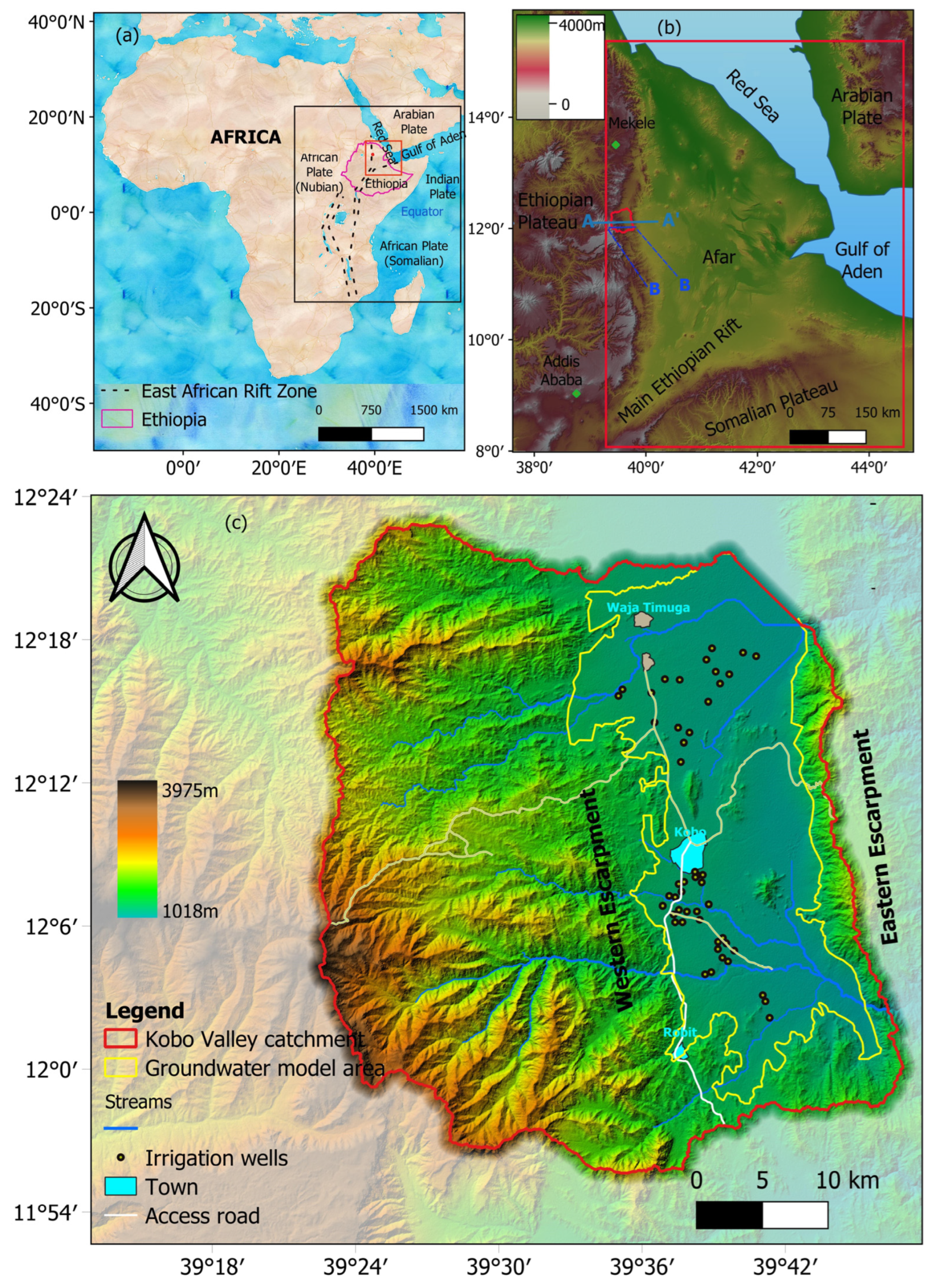
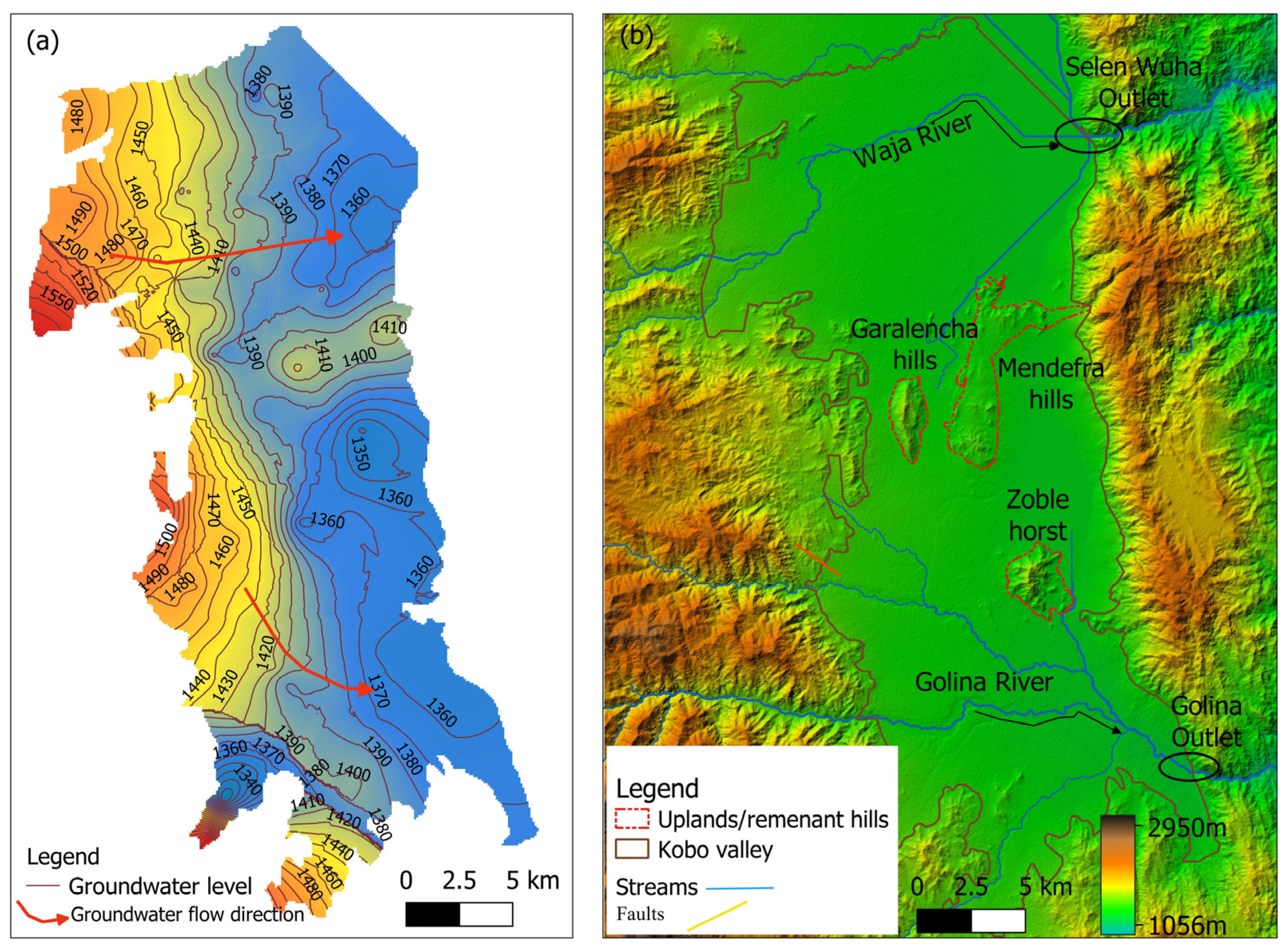
2.1. Description of Study Area
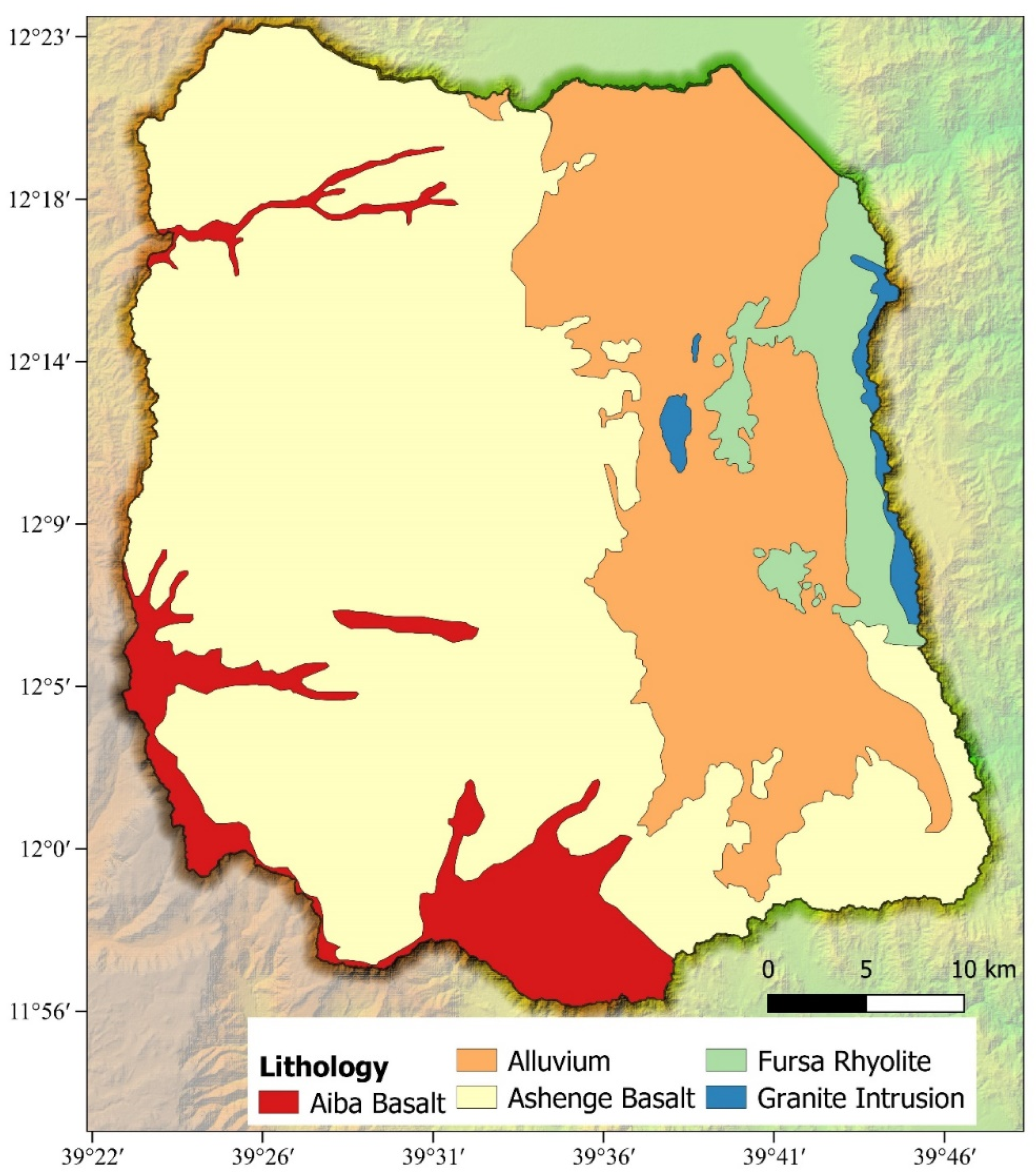
2.2. Geology of the Kobo Valley
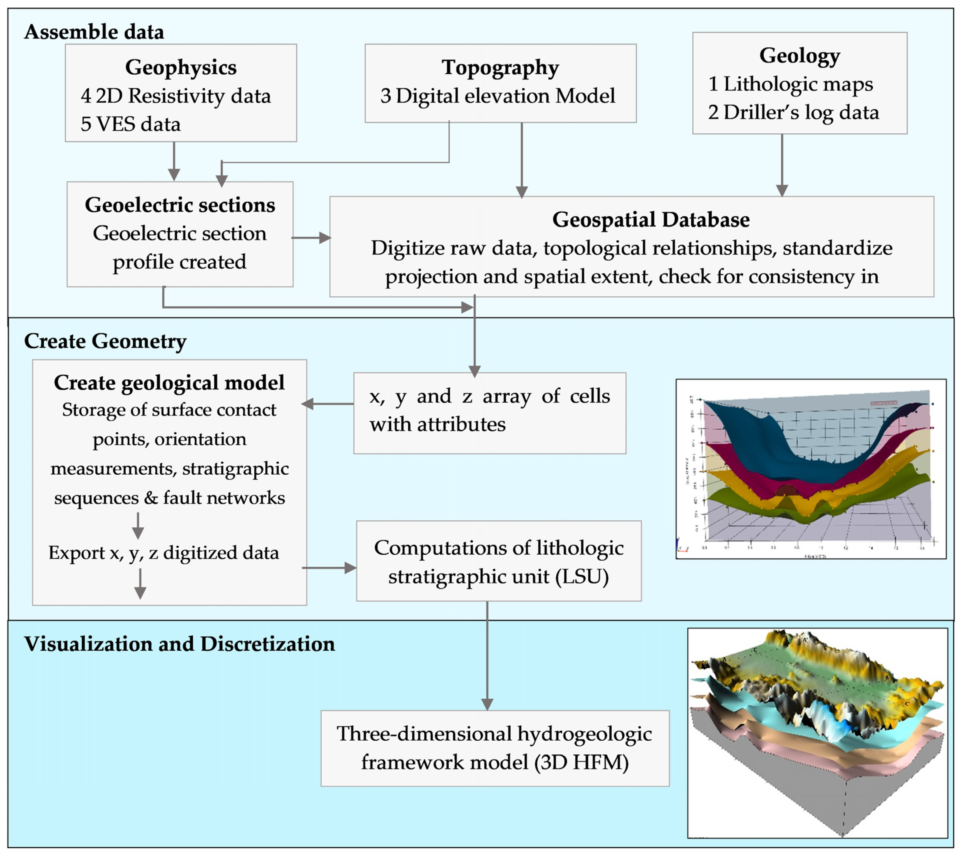
2.3. Data Collection and Processing
- Create a digitized geospatial database from the input data that contains all the raw data, topological relationships, standardized projection, and spatial extent;
- Define the spatial distribution of geological structures and discretize the 3D space regular grid geometry based on a potential-field interpolation method to define the spatial distribution of geological structures, such as layers, interfaces, and faults (computations of lithologic stratigraphic unit (LSU));
- Discretize and visualize an interactive 3D geological model using Python fundamental plotting library;
- Then, pre-process and analyze the driller’s log data to check whether they are consistent with the defined geometry and to identify the information that the contacts bring about the possible positions of the surface deviations.
2.4. VES Data
2.5. GemPy Modeling Approach
2.6. Model Performance Evaluation
3. Results and Discussion
3.1. Driller’s Log Lithology and VES Analysis
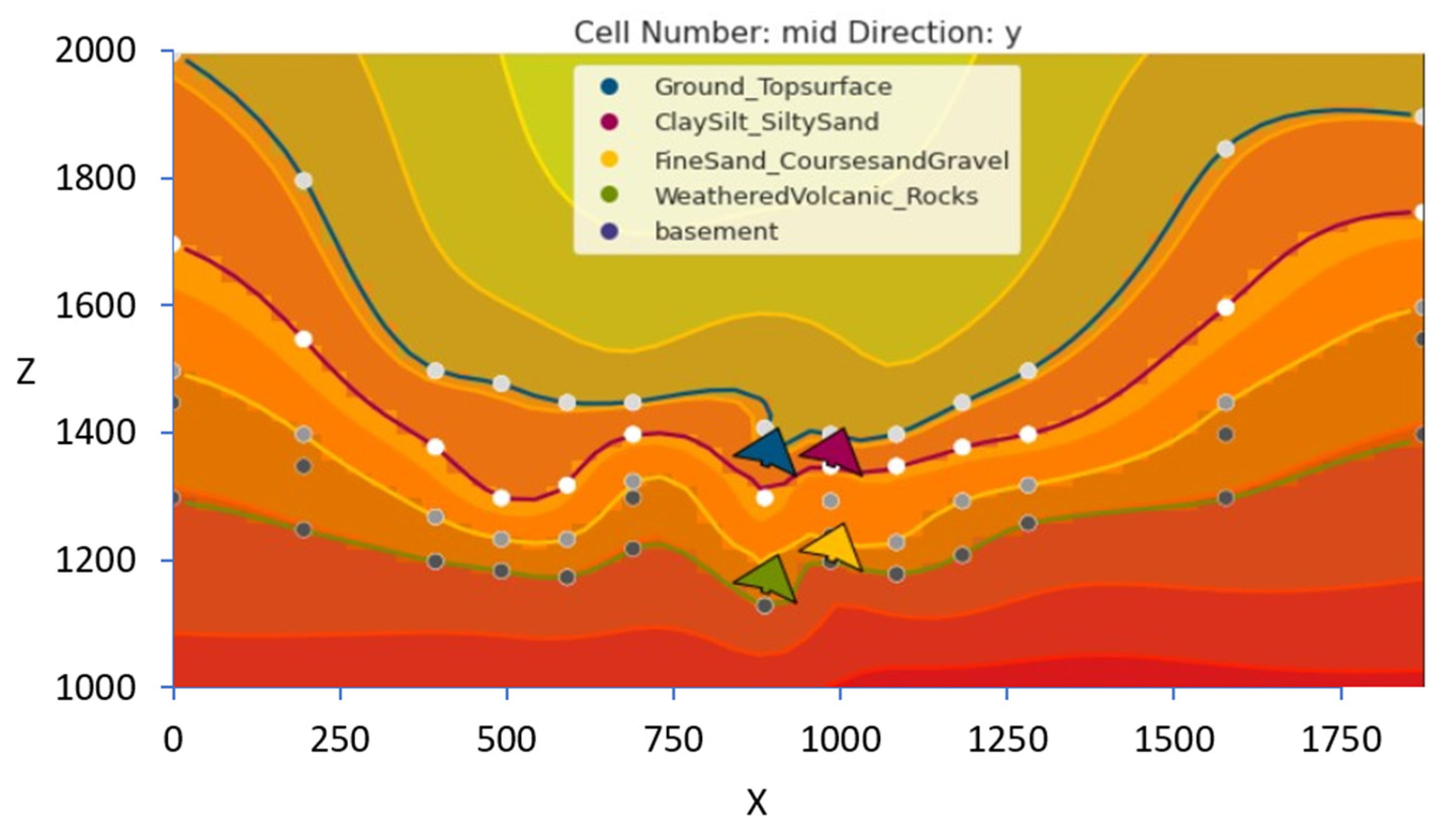
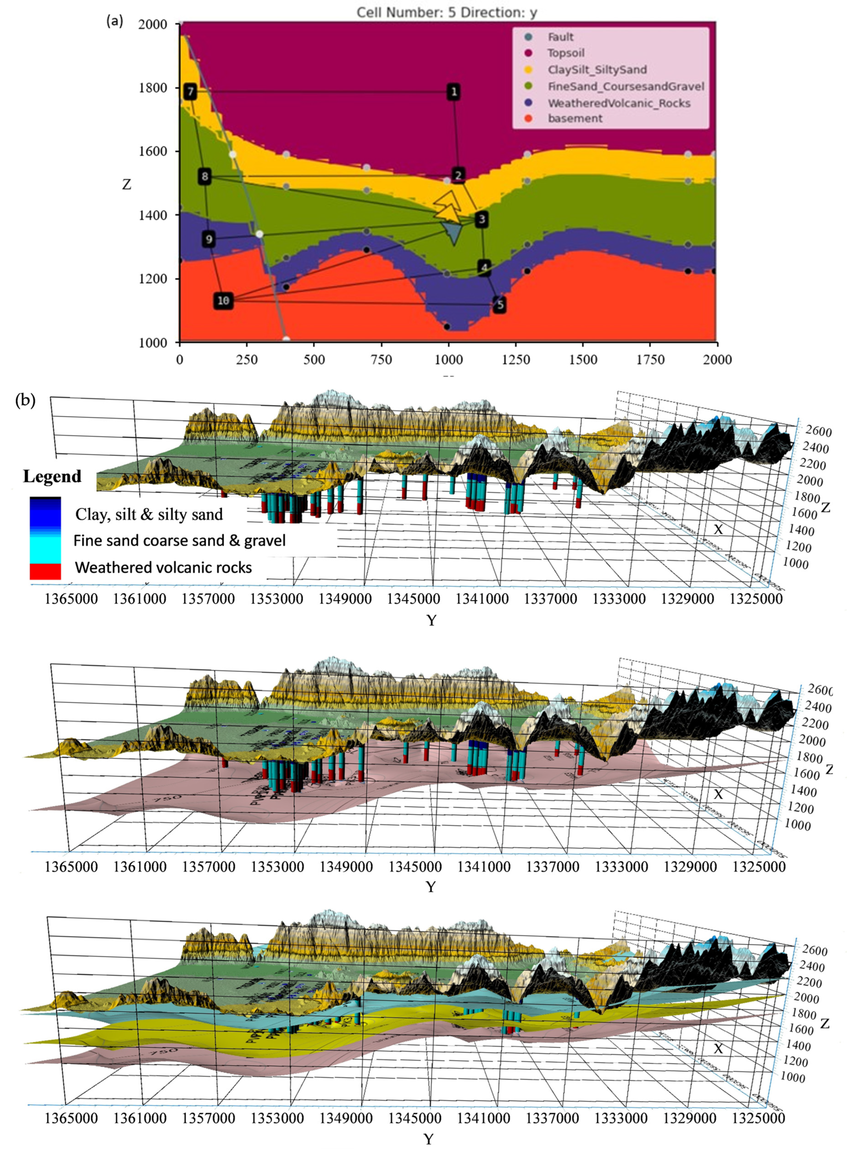
3.2. Three-Dimensional Hydrogeological Framework
3.3. Uncertainty in the GemPy Model
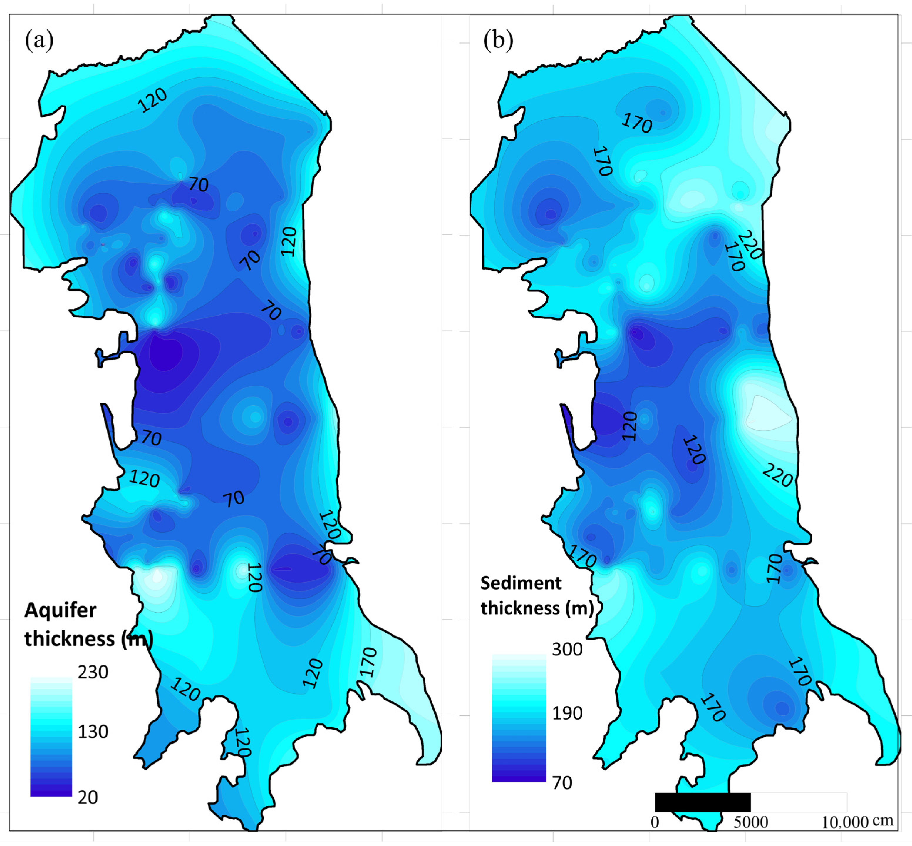
3.4. Kobo Valley Aquifer and Sediment Layer Visualization
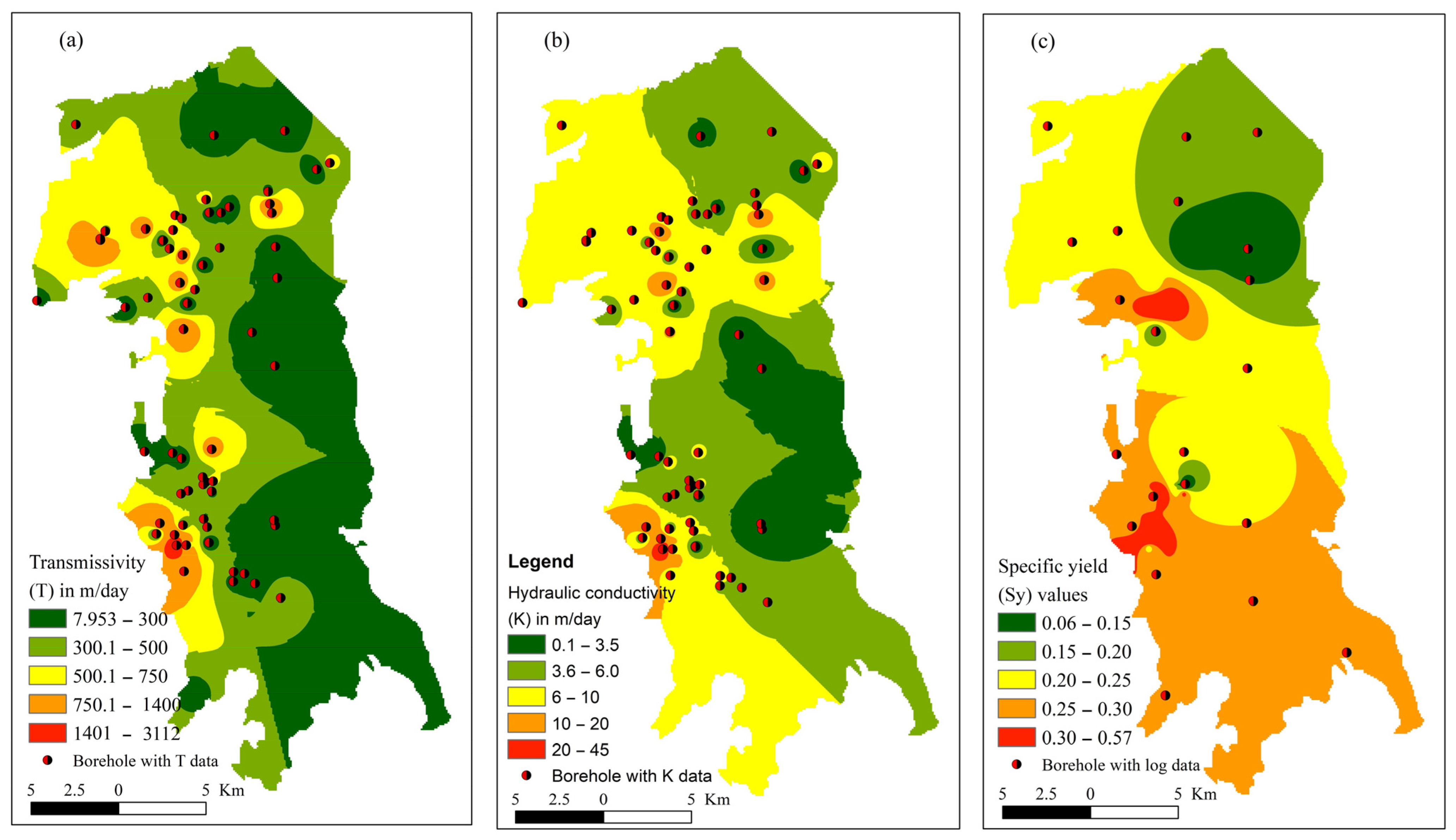
3.5. Hydraulic Properties of the Valley
3.6. Groundwater Flow System
3.7. Groundwater Storage in the Valley
4. Conclusions
Author Contributions
Funding
Data Availability Statement
Acknowledgments
Conflicts of Interest
Disclaimer
Appendix A. GemPy Codes


Appendix B. Summary of VES Measurement Survey Interpretation

| Profile | VES ID | Profile Layers and Lithology Identified |
|---|---|---|
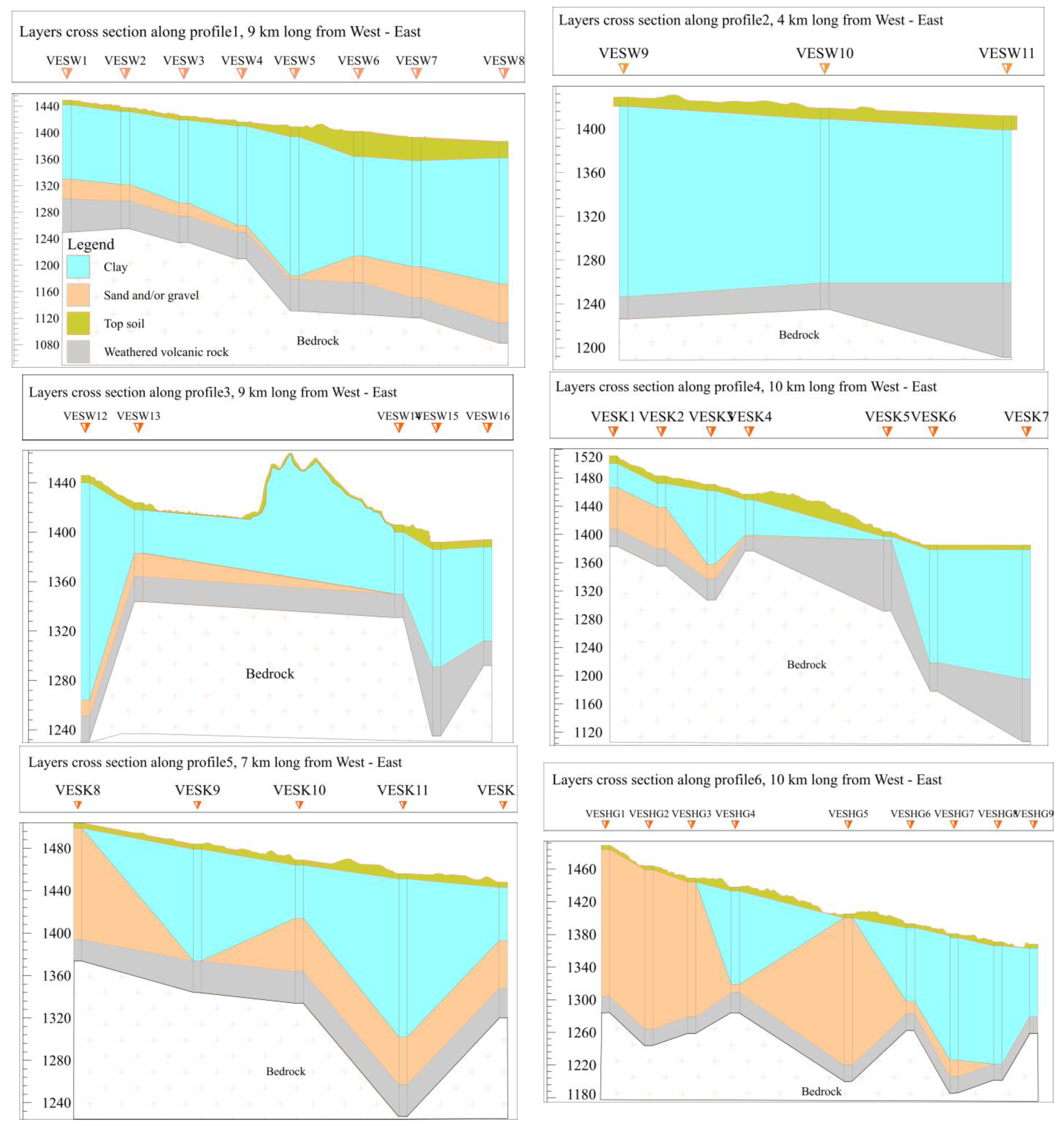
| Profile1 | VESW1 to VESW8 | Top soil (1 to 33 m), clay layer 112 m at VESW1 to 210 m thick at VESW5, sandy/gravel layer (5 m at VESW5 to 59 m thick at VESW8), weathered volcanic 50 m at VESW1 and 48 m at VESW5, bed rock |
| Profile2 | VESW9 to VESW11 | Top soil (1 to 8 m), clayey layer (174 m at VESW9 and 140 at VESW11), thin sand/gravel layer, weathered volcanic 24 m at VESW10 and 68 m thick at VESW11, bed rock |
| Profile3 | VESW12 to VESW16 | Very thin top soil, clay layer ranges from 76 m at VESW16 to 176 m at VESW12, gravel layer of 13 m at VESW13 to 19 m at VESW14, weathered rock of 19 m at VESW15 and 56 m at VESW14, bed rock |
| Profile4 | VESK1 to VESK7 | Top soil (2 to 6 m), sand/gravel layer at the western half at VESK 2 and 3 thickness of 59 m and 20.9 and clay at the eastern half and weathered volcanic at the center. Clay layer on western half has thickness of 33.5 m at VESK2 and 104 m at VESK3. The eastern clay layer is 160 m at VESK6 and 183 m at VESK7, weathered zone 24 m at VESK2 and 88.8 m at VESk7, bed rock |
| Profile5 | VESK8 to VESK12 | The sandy/gravel layer thickness varies from 105 m at VESK8 to 45 m at VESK12, the clay layer filling the central and eastern part of the profile is 105 m to 149 m at VESK12, weathered zone has thickness of 20 to 30 m, bed rock |
| Profile6 | VESHG1 to VESHG9 | Thick clay layer of max 150 m at VESHG7 and 114 m at VESHG4, sand/gravel layer with maximum thickness of 195 m at VESHG2 and minimum thickness at VESHG4 (10 m), third layer above the fresh bed rock is the weathered zone of 30 to 40 m. |
References
- Altchenko, Y.; Villholth, K.G. Mapping irrigation potential from renewable groundwater in Africa—A quantitative hydrological approach. Hydrol. Earth Syst. Sci. 2015, 19, 1055–1067. [Google Scholar] [CrossRef]
- Gaye, C.B.; Tindimugaya, C. Review: Challenges and opportunities for sustainable groundwater management in Africa. Hydrogeol. J. 2018, 27, 1099–1110. [Google Scholar] [CrossRef]
- MacDonald, A.; Adelana, S. Groundwater research issues in Africa. Appl. Groundw. Stud. Afr. 2008, 2008, 6152. [Google Scholar]
- Varga, M.d.L.; Schaaf, A.; Wellmann, F. GemPy 1.0: Open-source stochastic geological modeling and inversion. Geosci. Model Dev. 2019, 12, 1–32. [Google Scholar] [CrossRef]
- Stumpf, A.J.; Keefer, D.A.; Turner, A.K. Overview and history of 3-D modeling approaches. In Applied Multidimensional Geological Modeling: Informing Sustainable Human Interaction with the Shallow Subsurface; Turner, A.K., Kessler, H., van der Muelen, M.J., Eds.; John Wiley & Sons: New York, NY, USA, 2022; pp. 95–112. [Google Scholar]
- Van der Meulen, M.; Doornenbal, J.; Gunnink, J.; Stafleu, J.; Schokker, J.; Vernes, R.; van Geer, F.; van Gessel, S.; van Heteren, S.; van Leeuwen, R.; et al. 3D geology in a 2D country: Perspectives for geological surveying in the Netherlands. Neth. J. Geosci.-Geol. En Mijnb. 2013, 92, 217–241. [Google Scholar] [CrossRef]
- Gross, D.L. Geology for Planning in De Kalb County, Illinois. Champaign, IL: Illinois State Geological Survey; Environmental Geology Notes 33; Pioneer Publishing Company: Oak Park, IL, USA, 1970; p. 26. [Google Scholar]
- Hunt, C.S.A.; Kempton, J.P. Geology for Planning in De Witt County, Illinois. Champaign, IL: Illinois State Geological Survey; Environmental Geology Notes 83; Urbana publishing Company: Urbana, IL, USA, 1977; p. 42. [Google Scholar]
- Berg, R.C.A.; Greenpool, M.R. Stack-Unit Geologic Mapping: Color-Coded and Computer-Based Methodology; State Geological Survey, Circular: Champaign, IL, USA, 1993; Volume 552, p. 11. [Google Scholar]
- Jones, R.; McCaffrey, K.; Clegg, P.; Wilson, R.; Holliman, N.; Holdsworth, R.; Imber, J.; Waggott, S. Integration of regional to outcrop digital data: 3D visualisation of multi-scale geological models. Comput. Geosci. 2009, 35, 4–18. [Google Scholar] [CrossRef]
- Calcagno, P.; Chilès, J.; Courrioux, G.; Guillen, A. Geological modelling from field data and geological knowledge. Phys. Earth Planet. Inter. 2008, 171, 147–157. [Google Scholar] [CrossRef]
- Karlović, I.; Marković, T.; Vujnović, T.; Larva, O. Development of a Hydrogeological Conceptual Model of the Varaždin Alluvial Aquifer. Hydrology 2021, 8, 19. [Google Scholar] [CrossRef]
- Faunt, C. Numerical Model of the Hydrologic Landscape and Groundwater Flow in California’s Central Valley. In Groundwater Availability of the Central Valley Aquifer; USGS: Reston, VA, USA, 2009; pp. 121–212. [Google Scholar]
- Hanson, R.T.; Schmid, W.; Faunt, C.C.; Lear, J.; Lockwood, B. Integrated Hydrologic Model of Pajaro Valley, Santa Cruz and Monterey Counties, California; Scientific Investigations Report; U.S. Geological Survey: Reston, VA, USA, 2014; p. 180. [Google Scholar]
- Hanson, R.T.; Martin, P.; Koczot, K.M. Simulation of Ground-Water/Surface-Water Flow in the Santa Clara-Calleguas Ground-Water Basin, Ventura County, California; Water-Resources Investigations Report; U.S. Geological Survey: Sacramento, CA, USA, 2003. [Google Scholar]
- Faunt, C.C.; Belitz, K.; Hanson, R.T. Development of a three-dimensional model of sedimentary texture in valley-fill deposits of Central Valley, California, USA. Hydrogeol. J. 2010, 18, 625–649. [Google Scholar] [CrossRef]
- Knight, R.; Smith, R.; Asch, T.; Abraham, J.; Cannia, J.; Viezzoli, A.; Fogg, G. Mapping Aquifer Systems with Airborne Electromagnetics in the Central Valley of California. Ground Water 2018, 56, 893–908. [Google Scholar] [CrossRef]
- Caruso, P.; Ochoa, C.G.; Jarvis, W.T.; Deboodt, T. A Hydrogeologic Framework for Understanding Local Groundwater Flow Dynamics in the Southeast Deschutes Basin, Oregon, USA. Geosciences 2019, 9, 57. [Google Scholar] [CrossRef]
- Ben Saad, E.; Ben Alaya, M.; Taupin, J.-D.; Patris, N.; Chaabane, N.; Souissi, R. A Hydrogeological Conceptual Model Refines the Behavior of a Mediterranean Coastal Aquifer System: A Key to Sustainable Groundwater Management (Grombalia, NE Tunisia). Hydrology 2023, 10, 180. [Google Scholar] [CrossRef]
- Lázaro, J.M.; Navarro, J.Á.S.; Gil, A.G.; Romero, V.E. 3D-geological structures with digital elevation models using GPU programming. Comput. Geosci. 2014, 70, 138–146. [Google Scholar] [CrossRef]
- Cox, M.E.; James, A.; Hawke, A.; Raiber, M. Groundwater Visualisation System (GVS): A software framework for integrated display and interrogation of conceptual hydrogeological models, data and time-series animation. J. Hydrol. 2013, 491, 56–72. [Google Scholar] [CrossRef]
- Brandenburg, J.P. Geologic Frameworks for Groundwater Flow Models; 2020: The Groundwater Project; Groundwater Project: Guelph, ON, Canada, 2020. [Google Scholar]
- Raiber, M.; Webb, J.; Cendón, D.; White, P.; Jacobsen, G. Environmental isotopes meet 3D geological modelling: Conceptualising recharge and structurally-controlled aquifer connectivity in the basalt plains of south-western Victoria, Australia. J. Hydrol. 2015, 527, 262–280. [Google Scholar] [CrossRef]
- Hanson, R.T. Hydrologic framework of the Santa Clara Valley, California. Geosphere 2015, 11, 606–637. [Google Scholar] [CrossRef]
- Everett, R.R.; Gibbs, D.R.; Hanson, R.T.; Sweetkind, D.S.; Brandt, J.T.; Falk, S.E.; Harich, C.R. Geology, Water-Quality, Hydrology, and Geomechanics of the Cuyama Valley Groundwater Basin, California, 2008–12; Scientific Investigations Report; U.S. Geological Survey: Reston, VA, USA, 2013; p. 76. [Google Scholar]
- Sweetkind, D.S.; Faunt, C.C.; Hanson, R.T. Construction of 3-D Geologic Framework and Textural Models for Cuyama Valley Groundwater Basin, California; U.S. Geological Survey Scientific Investigations Report 2013–5127; U.S. Geological Survey: Reston, VA, USA, 2013; p. 46. [Google Scholar]
- Wentworth, C.M.; Jachens, R.C.; Williams, R.A.; Tinsley, J.C., III; Hanson, R.T. Physical Subdivision and Description of the Water-Bearing Sediments of the Santa Clara Valley, California; Scientific Investigations Report; USGS: Reston, VA, USA, 2015; p. 84. [Google Scholar]
- Sweetkind, D.S. Three-Dimensional Hydrogeologic Framework Model of the Rio Grande Transboundary Region of New Mexico and Texas, USA, and Northern Chihuahua, Mexico; Scientific Investigations Report; USGS: Reston, VA, USA, 2017; p. 61. [Google Scholar]
- Belcher, W.R.; Sweetkind, D.S.; Faunt, C.C.; Pavelko, M.T.; Hill, M.C. An Update of the Death Valley regional Groundwater Flow System Transient Model, Nevada and California; Scientific Investigations Report; USGS: Reston, VA, USA, 2017. [Google Scholar]
- Shishaye, H.A.; Tait, D.R.; Befus, K.M.; Maher, D.T.; Reading, M.J.; Jeffrey, L.; Tewolde, T.G.; Asfaw, A.T. Development of an improved hydrogeological and hydro-geochemical conceptualization of a complex aquifer system in Ethiopia. Hydrogeol. J. 2020, 28, 2727–2746. [Google Scholar] [CrossRef]
- Bashir, I.Y.; Izham, M.Y.; Main, R. Vertical Electrical Sounding Investigation of Aquifer Composition and Its Potential to Yield Groundwater in Some Selected Towns in Bida Basin of North Central Nigeria. J. Geogr. Geol. 2014, 6, 60–69. [Google Scholar] [CrossRef]
- Soomro, A.; Qureshi, A.L.; Jamali, M.A.; Ashraf, A. Groundwater investigation through vertical electrical sounding at hilly area from Nooriabad toward Karachi. Acta Geophys. 2019, 67, 247–261. [Google Scholar] [CrossRef]
- Iserhien-Emekeme, R.; Ofomola, M.O.; Bawallah, M.; Anomohanran, O. Lithological Identification and Underground Water Conditions in Jeddo Using Geophysical and Geochemical Methods. Hydrology 2017, 4, 42. [Google Scholar] [CrossRef]
- Jiang, Y.; Sun, M.; Yang, C. A Generic Framework for Using Multi-Dimensional Earth Observation Data in GIS. Remote Sens. 2016, 8, 382. [Google Scholar] [CrossRef]
- Dynamic Graphics, Inc. EarthVision. 2020. Available online: http://www.dgi.com/earthvision/evmain.html (accessed on 10 June 2022).
- ARANZ Geo Limited. Leapfrog3D. 2015. Available online: http://www.leapfrog3d.com/ (accessed on 18 May 2022).
- GOCAD. Gocad Research Group Mira Geoscience. 2022. Available online: https://mirageoscience.com/mining-industry-software/gocad-mining-suite/ (accessed on 12 April 2022).
- Petra. IHS Petra. 2022. Available online: https://www.spglobal.com/commodityinsights/en/ci/products/petra-geological-analysis.html (accessed on 24 July 2022).
- Rockworks, Rockware, Inc. 2022. Available online: https://www.rockware.com (accessed on 10 July 2022).
- HydroGeoAnalyst, Schlumberger Water Services. 2011. Available online: https://www.waterloohydrogeologic.com/products/hydro-geoanalyst/ (accessed on 2 August 2022).
- Velasco, V.R.; Gogu, C.R.; Vázquez-Suñé, E.; Garriga, A.; Ramos, E.; Riera, J.; Alcaraz, M. The use of GIS-based 3D geological tools to improve hydrogeological models of sedimentary media in an urban environment. Environ. Earth Sci. 2013, 68, 2145–2162. [Google Scholar] [CrossRef]
- Rossetto, R.; De Filippis, G.; Borsi, I.; Foglia, L.; Cannata, M.; Criollo, R.; Vázquez-Suñé, E. Integrating free and open source tools and distributed modelling codes in GIS environment for data-based groundwater management. Environ. Model. Softw. 2018, 107, 210–230. [Google Scholar] [CrossRef]
- Bittner, D.; Rychlik, A.; Klöffel, T.; Leuteritz, A.; Disse, M.; Chiogna, G. A GIS-based model for simulating the hydrological effects of land use changes on karst systems—The integration of the LuKARS model into FREEWAT. Environ. Model. Softw. 2020, 127, 104682. [Google Scholar] [CrossRef]
- Wellmann, F.; Caumon, G. 3-D Structural Geological Models: Concepts, Methods, and Uncertainties; Elsevier: Amsterdam, The Netherlands, 2018; pp. 1–121. [Google Scholar]
- Mitášová, H.; Mitáš, L. Interpolation by regularized spline with tension: I. Theory and implementation. Math. Geol. 1993, 25, 641–655. [Google Scholar] [CrossRef]
- Matheron, G. Principles of geostatistics. Econ. Geol. 1963, 58, 1246–1266. [Google Scholar] [CrossRef]
- MacDonald, A.M.; Bonsor, H.C.; Dochartaigh, B.É.Ó.; Taylor, R.G. Quantitative maps of groundwater resources in Africa. Environ. Res. Lett. 2012, 7, 024009. [Google Scholar] [CrossRef]
- Cobbing, J.; Hiller, B. Waking a sleeping giant: Realizing the potential of groundwater in Sub-Saharan Africa. World Dev. 2019, 122, 597–613. [Google Scholar] [CrossRef]
- Mekonen, S.S.; Boyce, S.E.; Mohammed, A.K.; Flint, L.; Flint, A.; Disse, M. Recharge Estimation Approach in a Data-Scarce Semi-Arid Region, Northern Ethiopian Rift Valley. Sustainability 2023, 15, 15887. [Google Scholar] [CrossRef]
- Tadesse, N.; Nedaw, D.; Woldearegay, K.; Gebreyohannes, T. Groundwater Management for Irrigation in the Raya and Kobo Valleys, Northern Ethiopia. Int. J. Earth Sci. Eng. 2015, 8, 36–46. [Google Scholar]
- Sisay Mengesha, G. Food Security Status of Peri-Urban Modern Small Scale Irrigation Project Beneficiary Female Headed Households in Kobo Town, Ethiopia. J. Food Secur. 2017, 5, 259–272. [Google Scholar] [CrossRef]
- Ayenew, T.; GebreEgziabher, M.; Kebede, S.; Mamo, S. Integrated assessment of hydrogeology and water quality for groundwater-based irrigation development in the Raya Valley, northern Ethiopia. Water Int. 2013, 38, 480–492. [Google Scholar] [CrossRef]
- Adane, G.W. Groundwater Modelling and Optimization of Irrigation Water Use Efficiency to Sustain Irrigation in Kobo Valley, Ethiopia; UNESCO-IHE Institute for Water Education: Delft, The Netherlands, 2014. [Google Scholar]
- Zwaan, F.; Corti, G.; Keir, D.; Sani, F. A review of tectonic models for the rifted margin of Afar: Implications for continental break-up and passive margin formation. J. Afr. Earth Sci. 2019, 164, 103649. [Google Scholar] [CrossRef]
- Beyene, A.; Abdelsalam, M.G. Tectonics of the Afar Depression: A review and synthesis. J. Afr. Earth Sci. 2005, 41, 41–59. [Google Scholar] [CrossRef]
- Corti, G.; Bastow, I.D.; Keir, D.; Pagli, C.; Baker, E. Rift-Related Morphology of the Afar Depression. In Landscapes and Landforms of Ethiopia; Springer Science and Business Media: Dordrecht, The Netherlands, 2015; pp. 251–274. [Google Scholar]
- Barberi, F.; Santacroce, R. The Afar Stratoid Series and the magmatic evolution of East African rift system. Bull. de la Société Géologique de Fr. 1980, S7-XXII, 891–899. [Google Scholar] [CrossRef]
- Stab, M.; Bellahsen, N.; Pik, R.; Quidelleur, X.; Ayalew, D.; Leroy, S. Modes of rifting in magma-rich settings: Tectono-magmatic evolution of Central Afar. Tectonics 2016, 35, 2–38. [Google Scholar] [CrossRef]
- Corti, G. Continental rift evolution: From rift initiation to incipient break-up in the Main Ethiopian Rift, East Africa. Earth-Sci. Rev. 2009, 96, 1–53. [Google Scholar] [CrossRef]
- Zwaan, F.; Corti, G.; Sani, F.; Keir, D.; Muluneh, A.A.; Illsley-Kemp, F.; Papini, M. Structural Analysis of the Western Afar Margin, East Africa: Evidence for Multiphase Rotational Rifting. Tectonics 2020, 39, e2019TC006043. [Google Scholar] [CrossRef]
- Hammond, J.O.S.; Kendall, J.-M.; Stuart, G.W.; Keir, D.; Ebinger, C.; Ayele, A.; Belachew, M. The nature of the crust beneath the Afar triple junction: Evidence from receiver functions. Geochem. Geophys. Geosyst. 2011, 12. [Google Scholar] [CrossRef]
- EGS, Ethiopian Geological Study, Government Document. 2012. Available online: https://docplayer.net/133114738-Geological-survey-of-ethiopia.html (accessed on 22 July 2022).
- ECDSWC, Ethiopian Construction Design and Supervision Works Corporation, Government Document. 2021. Available online: https://waterpip.un-ihe.org/ethiopian-construction-design-and-supervision-works-corporation (accessed on 22 July 2022).
- MCE, M.C.E. Hydrogeological and Geophysical Investigation Report of Kobo—Girana irrigation project by Metaferia Consulting Egneers. Government Document. 2009. Available online: https://www.metaferia.com/portfolio-4-columns-no-space/irrigation-agro-industry/ (accessed on 22 July 2022).
- Program, I.W. Program for Vertical Electrical Sounding Curves 1-D Interpreting along a Single Profile; Department of geophysics, Geological Faculty, Moscow University: Moscow, Russia, 2000. [Google Scholar]
- Ibuot, J.; Akpabio, G.; George, N. A Survey of the Repository of Groundwater Potential and Distribution Using Geoelectrical Resistivity Method in Itu Local Government Area (L.G.A); Open Geosciences: Akwa Ibom State, Southern Nigeria, 2013; Volume 5. [Google Scholar]
- Okoyeh, E.I.; Akpan, A.E.; Egboka, B.C.E.; Okeke, H.I. An Assessment of the Influences of Surface and Subsurface Water Level Dynamics in the Development of Gullies in Anambra State, Southeastern Nigeria. Earth Interact. 2014, 18, 1–24. [Google Scholar] [CrossRef]
- González-Álvarez, I.; Ley-Cooper, A.Y.; Salama, W. A geological assessment of airborne electromagnetics for mineral exploration through deeply weathered profiles in the southeast Yilgarn Cratonic margin, Western Australia. Ore Geol. Rev. 2016, 73, 522–539. [Google Scholar] [CrossRef]
- Loke, M.H. 2-D and 3-D Electrical Imaging Surveys. 2021. Available online: https://www.researchgate.net/publication/264739285_Tutorial_2-D_and_3-D_Electrical_Imaging_Surveys (accessed on 22 July 2022).
- Cyril, A.G. Interpretation of Geolectric Pseudo Section and Seismic Refraction Tomography with Borehole Logs Carried out across a Functional Borehole at Garaje-Kagoro Area of Kaduna Northwestern Nigeria. NIPES J. Sci. Technol. Res. 2020, 2, 124. [Google Scholar] [CrossRef]
- Lajaunie, C.; Courrioux, G.; Manuel, L. Foliation Fields and 3D Cartography in Geology: Principles of a Method Based on Potential Interpolation. Math. Geol. 1997, 29, 4. [Google Scholar] [CrossRef]
- Salvatier, J.; Wiecki, T.V.; Fonnesbeck, C. Probabilistic programming in Python using PyMC3. PeerJ Comput. Sci. 2016, 2, e55. [Google Scholar] [CrossRef]
- Theano Development Team. A Python Framework for Fast Computation of Mathematical Expressions; Montreal Institute for Learning Algorithms (MILA), Université de Montréal: Montréal, QC, Canada, 2016. [Google Scholar]
- Mckinney, W. pandas: A Foundational Python Library for Data Analysis and Statistics, Python for High Performance and Scientific Computing. ResearchGate 2011, 14, 1–9. [Google Scholar]
- Schroeder, W.; Martin, K.; Lorensen, B. The Visualization Toolkit an Object-Oriented Approach to 3D Graphics. Kitware 2004, 2004. [Google Scholar]
- Hunter, J.D. Matplotlib: A 2D graphics environment. Comput. Sci. Eng. 2007, 9, 90–95. [Google Scholar] [CrossRef]
- Walt, S.V.D.; Colbert, S.C.; Varoquaux, G. The NumPy Array: A Structure for Efficient Numerical Computation. Comput. Sci. Eng. 2011, 13, 22–30. [Google Scholar] [CrossRef]
- Lark, R.; Mathers, S.; Thorpe, S.; Arkley, S.; Morgan, D.; Lawrence, D. A statistical assessment of the uncertainty in a 3D geological framework model. Br. Geol. Surv. 2013, 124, 946–958. [Google Scholar]
- Wellmann, J.F.; Horowitz, F.G.; Schill, E.; Regenauer-Lieb, K. Towards incorporating uncertainty of structural data in 3D geological inversion. Tectonophysics 2010, 490, 141–151. [Google Scholar] [CrossRef]
- Koller, D.; Friedman, N. Probabilistic Graphical Models: Principles and Techniques Adaptive Computation and Machine Learning; The MIT Press: Cambridge, MA, USA, 2009. [Google Scholar]
- Wellmann, J.F.; Regenauer-Lieb, K. Uncertainties have a meaning: Information entropy as a quality measure for 3-D geological models. Tectonophysics 2012, 526–529, 207–216. [Google Scholar] [CrossRef]
- Schweizer, D.; Blum, P.; Butscher, C. Uncertainty assessment in 3-D geological models of increasing complexity. Solid Earth 2017, 8, 515–530. [Google Scholar] [CrossRef]
- Martin, J.; Adana, D.D.R.D.; Asuero, A.G. Fitting Models to Data: Residual Analysis, a Primer. In Uncertainty Quantification and Model Calibration; InTechOpen Publisher: London, UK, 2017. [Google Scholar]
- Bear, J. Hydraulics of Groundwater, McGraw-Hill Series in Water Resources and Environmental Engineering; McGraw-Hill: New York, NY, USA, 1979; Available online: https://www.perlego.com/book/110730/hydraulics-of-groundwater-pdf (accessed on 22 July 2022).
- Freeze, R.A.; Cherry, J.A. Groundwater; Prentice-Hall Inc.: Englewood Cliffs, NY, USA, 1979; Volume 7632, p. 604. [Google Scholar]
- Todd, D.K. Groundwater Hydrology; Agrosy Publishing: 1959. Available online: https://old.amu.ac.in/emp/studym/99994128.pdf (accessed on 22 July 2022).
- Heath, R.C. Basic ground-water hydrology. In Water Supply Paper; USGS: Reston, VA, USA, 1983; p. 91. [Google Scholar]
- Scanlon, B.R.; Longuevergne, L.; Long, D. Ground referencing GRACE satellite estimates of groundwater storage changes in the California Central Valley, USA. Water Resour. Res. 2012, 48. [Google Scholar] [CrossRef]
- Wahyuni, S.; Oishi, S.; Sunada, K. The Estimation of the Groundwater Storage and Its Distribution in Uzbekistan. Proc. Hydraul. Eng. 2008, 52, 31–36. [Google Scholar] [CrossRef]
- Evans, S.W.; Jones, N.L.; Williams, G.P.; Ames, D.P.; Nelson, E.J. Groundwater Level Mapping Tool: An open source web application for assessing groundwater sustainability. Environ. Model. Softw. 2020, 131, 104782. [Google Scholar] [CrossRef]
- Bhanja, S.N.; Rodell, M.; Li, B.; Saha, D.; Mukherjee, A. Spatio-temporal variability of groundwater storage in India. J. Hydrol. 2017, 544, 428–437. [Google Scholar] [CrossRef]
- Todd, D.K.; Mays, L.W. Groundwater Hydrology, 3rd ed.; John Wiley & Sons, Inc.: New York, NY, USA, 2005. [Google Scholar]
- ECDSWC. Kobo Chefa Groundwater Resource Evaluation, Assessment and Test Wells Drilling Supervision Project, Volume-I: Updating the Groundwater Potential Evaluation of Kobo Area; Government Document; Addis Ababa, Ethiopia, 2018; Available online: https://waterpip.un-ihe.org/ethiopian-construction-design-and-supervision-works-corporation (accessed on 22 July 2022).
- MCE. Metaferia Consulting Engineers; Hydrogeological Investigation Report; Ministry of Water Resources of Ethiopia: Addis Ababa, Ethiopia, 2009. [Google Scholar]


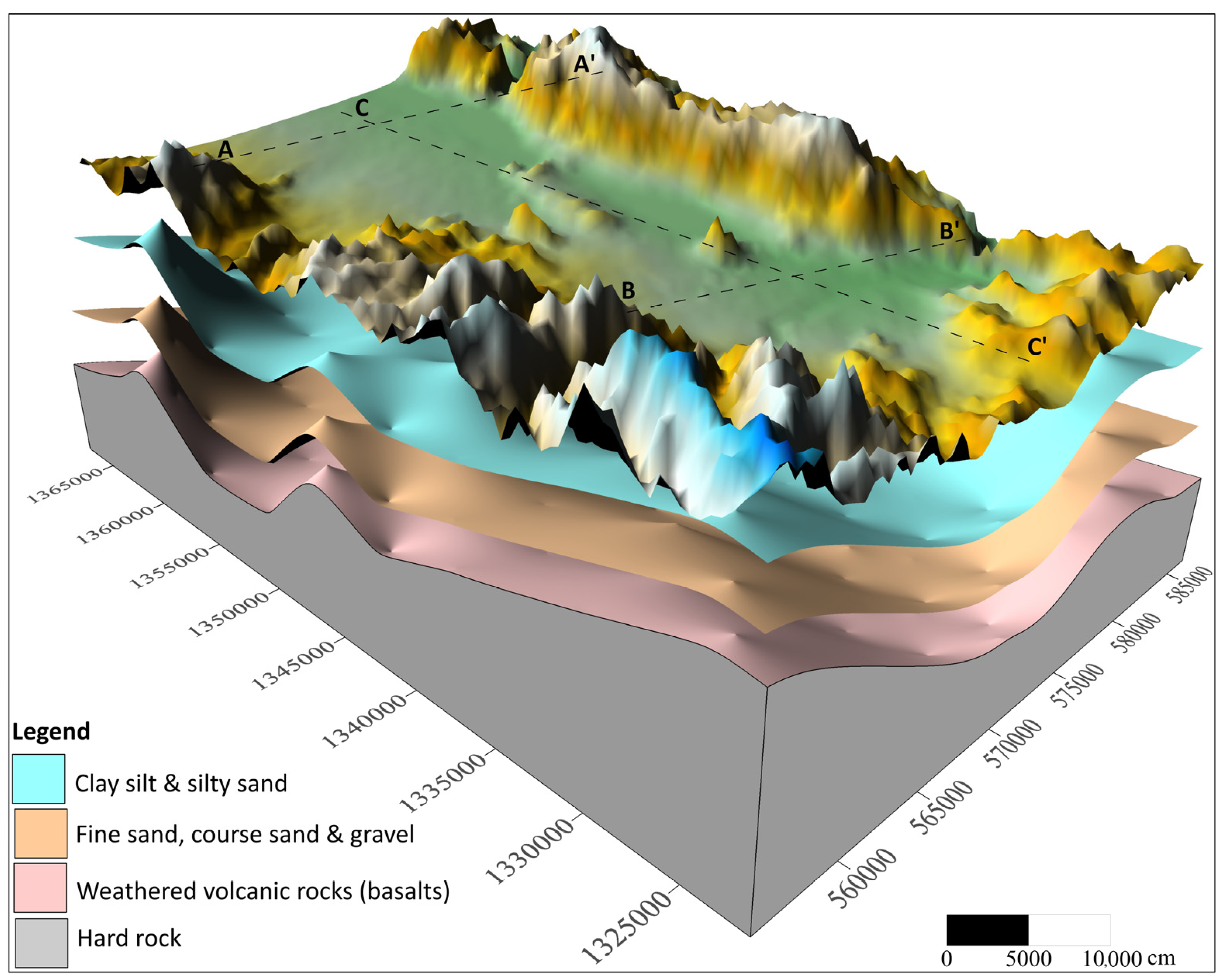

| Hydrogeologic Stratigraphic Unit (HSU) | HSU Order | Volume of Unit in m3 |
|---|---|---|
| Clay, silt, and silty sand | First (top) layer | 38.21 × 10⁹ |
| Fine sand, coarse sand, and gravel | Second layer | 26.79 × 10⁹ |
| Weathered volcanic rock (basalts) | Third layer 1 | 17.22 × 10⁹ |
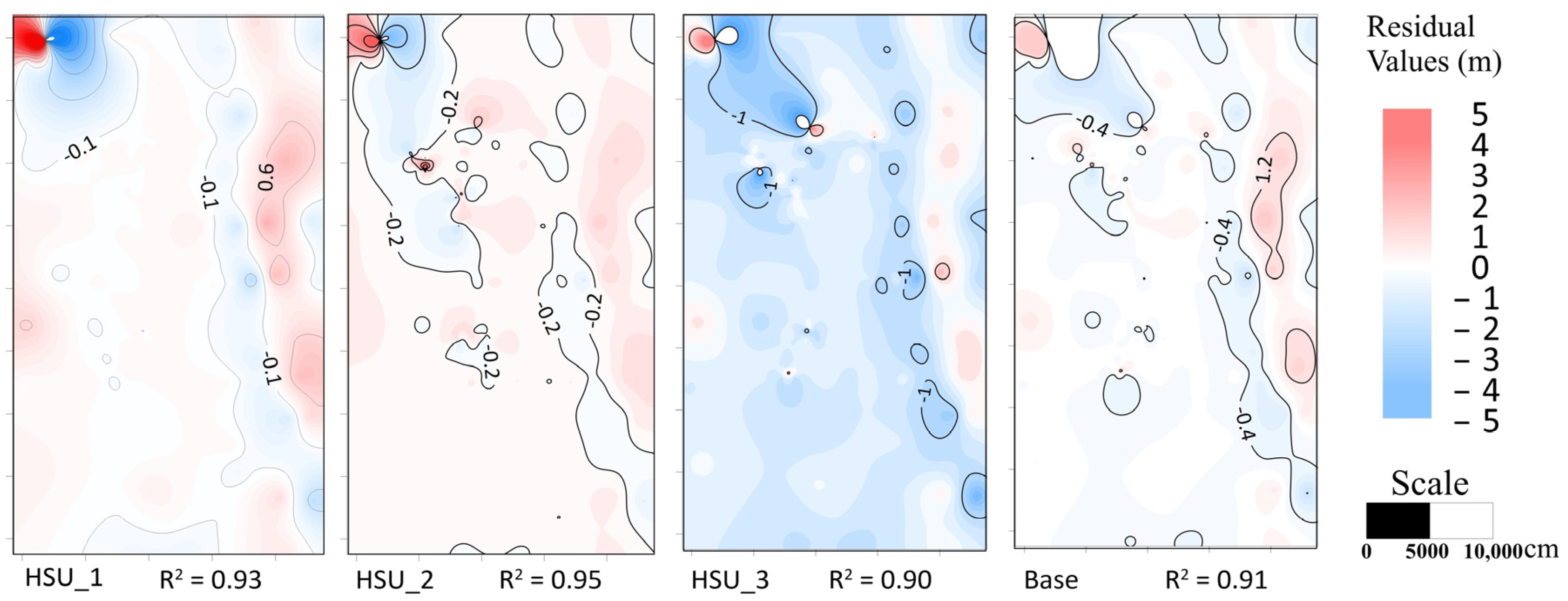
| Minimum (m) | Maximum (m) | Mean (m) | SE (m) | SD (m) | R2 | HSU | Description |
|---|---|---|---|---|---|---|---|
| −5.68 | 7.71 | 0.01 | 0.08 | 0.91 | 0.93 | HSU_1 | top of clay, silt, and silty sand layer |
| −7.52 | 7.84 | -0.58 | 0.60 | 6.76 | 0.95 | HSU_2 | bottom of clay, silt, and silty sand layer, and top of fine sand, coarse sand, and gravel layer |
| −9.68 | 7.71 | 0.01 | 0.10 | 1.01 | 0.90 | HSU_3 | bottom of fine sand, coarse sand, and gravel layer and top of basalts layer |
| −6.14 | 8.32 | 0.04 | 0.10 | 1.12 | 0.91 | Base | top of hard rock |
Disclaimer/Publisher’s Note: The statements, opinions and data contained in all publications are solely those of the individual author(s) and contributor(s) and not of MDPI and/or the editor(s). MDPI and/or the editor(s) disclaim responsibility for any injury to people or property resulting from any ideas, methods, instructions or products referred to in the content. |
© 2023 by the authors. Licensee MDPI, Basel, Switzerland. This article is an open access article distributed under the terms and conditions of the Creative Commons Attribution (CC BY) license (https://creativecommons.org/licenses/by/4.0/).
Share and Cite
Mekonen, S.S.; Boyce, S.E.; Mohammed, A.K.; Disse, M. Using an Open-Source Tool to Develop a Three-Dimensional Hydrogeologic Framework of the Kobo Valley, Ethiopia. Geosciences 2024, 14, 3. https://doi.org/10.3390/geosciences14010003
Mekonen SS, Boyce SE, Mohammed AK, Disse M. Using an Open-Source Tool to Develop a Three-Dimensional Hydrogeologic Framework of the Kobo Valley, Ethiopia. Geosciences. 2024; 14(1):3. https://doi.org/10.3390/geosciences14010003
Chicago/Turabian StyleMekonen, Sisay S., Scott E. Boyce, Abdella K. Mohammed, and Markus Disse. 2024. "Using an Open-Source Tool to Develop a Three-Dimensional Hydrogeologic Framework of the Kobo Valley, Ethiopia" Geosciences 14, no. 1: 3. https://doi.org/10.3390/geosciences14010003
APA StyleMekonen, S. S., Boyce, S. E., Mohammed, A. K., & Disse, M. (2024). Using an Open-Source Tool to Develop a Three-Dimensional Hydrogeologic Framework of the Kobo Valley, Ethiopia. Geosciences, 14(1), 3. https://doi.org/10.3390/geosciences14010003