Article

Interpretation of Hyperspectral Shortwave Infrared Core Scanning Data Using SEM-Based Automated Mineralogy: A Machine Learning Approach

Center to Advance the Science of Exploration to Reclamation in Mining, Colorado School of Mines, Golden, CO 80401, USA
*
Author to whom correspondence should be addressed.
Geosciences 2023, 13(7), 192; https://doi.org/10.3390/geosciences13070192
Submission received: 20 April 2023 / Revised: 30 May 2023 / Accepted: 15 June 2023 / Published: 24 June 2023
(This article belongs to the Special Issue Machine Learning in Applied Earth Science)

Abstract

:
Understanding the mineralogy and geochemistry of the subsurface is key when assessing and exploring for mineral deposits. To achieve this goal, rapid acquisition and accurate interpretation of drill core data are essential. Hyperspectral shortwave infrared imaging is a rapid and non-destructive analytical method widely used in the minerals industry to map minerals with diagnostic features in core samples. In this paper, we present an automated method to interpret hyperspectral shortwave infrared data on drill core to decipher major felsic rock-forming minerals using supervised machine learning techniques for processing, masking, and extracting mineralogical and textural information. This study utilizes a co-registered training dataset that integrates hyperspectral data with quantitative scanning electron microscopy data instead of spectrum matching using a spectral library. Our methodology overcomes previous limitations in hyperspectral data interpretation for the full mineralogy (i.e., quartz and feldspar) caused by the need to identify spectral features of minerals; in particular, it detects the presence of minerals that are considered invisible in traditional shortwave infrared hyperspectral analysis.

1. Introduction

In the mining industry, knowledge of the mineralogical makeup of ore and host rock units is critical at many stages of a project’s life cycle, ranging from early exploration to production and remediation. Hyperspectral imaging is currently the method of choice in the mining industry, as it allows mineralogical analysis of large amounts of drill core in a short period of time, permitting operators to acquire mineralogical data in nearly real time during exploration and resource definition [1,2,3,4]. Hyperspectral imaging of drill core typically involves measuring the absorption of light in the visible to near-infrared (VNIR) and shortwave infrared (SWIR). The composition of each measured pixel in the core scan can then be determined by spectral matching and feature fitting algorithms as part of data postprocessing.
However, significant problems arise because spectra are often produced by spectral overlap of different minerals present in each pixel, and common minerals such as garnet, olivine, feldspar, and quartz, as well as many oxide and sulfide minerals, lack well defined diagnostic VNIR-SWIR spectral features [3,4] and are undetectable by such methods. Moreover, the spectrally dominant mineral in a measured pixel may not be the dominant mineral in the pixel. To overcome these limitations, we propose an automated method of spectral interpretation that extracts associations between hyperspectral and quantitative automated mineralogy data using supervised machine learning techniques. Our proposed methodology does not require the minerals to have VNIR-SWIR hyperspectral diagnostic absorption features to be identified, nor does it require the use of spectral libraries, which may or may not be appropriate to identify minerals occurring at a given study site. Instead the method learns identifying features from data.
Using an automated approach based on learning from the available data helps to reduce the subjectivity in the analysis and to avoid mineral identification based solely on spectral predominance. The basic idea is to use supervised learning to automate processes that usually rely on experts’ knowledge, such as defining masks for core measured in boxes and feature identification in spectra. Expert knowledge is not ignored, as it is of great value and can be incorporated in training of the neural networks. For instance, in our approach (Section 3) we use it to help the network learn masking of drill core boxes.
The two main goals of our work are to develop methods to (i) automate the construction of masks, which are otherwise hand-drawn by visual inspection of the images obtained from the drill core boxes and (ii) extract mineral information from hyperspectral data given ground truth information obtained from scanning electron microscope (SEM) data, including minerals such as quartz and feldspar that are traditionally considered invisible in SWIR hyperspectral analysis. For both tasks, we use supervised machine learning techniques based on convolutional neural networks (CNN). They are supervised because in order to construct masks the networks use hand-drawn masks to learn the masking, while the mineral identification networks learn to identify features in hyperspectral data using the mineralogy from SEM data. To achieve these objectives (and with the final goal of eventually obtaining a fully automated processing tool), we use supervised learning and other machine learning techniques for the pre- and postprocessing steps required for each of the main tasks.
Following this introduction, the remaining parts of this paper describe the developed methodology and its applications. Figure 1 summarizes the basic flow of the analysis. In Section 2, we describe the data used for our study as well as the basic data processing steps used prior to analysis. Supervised learning methods for the construction of masks are described in Section 3. The machine learning methods used for mineral identification are discussed in Section 4. Section 3 and Section 4 include descriptions of further data processing steps as well as the results obtained by applying our methodology to the data. Finally, the paper concludes in Section 5 with a summary and comments.

2. Data and Processing

Our machine learning methods were developed and tested using drill core from the Castle Mountain low-sulfidation epithermal gold deposit, which is located on the margin of the Colorado River extensional corridor in California [5,6]. The deposit has a total endowment of over 150 metric tonnes of gold, and is hosted in pervasively altered volcanic rocks [7].
Samples for analysis were collected from an exploration diamond drill hole in the southern part of the deposit area (drill hole CMM-111, intersecting 637.5 m of dominantly felsic lavas and volcaniclastic rocks). One interval of rhyolite was chosen for subsampling due to its relative lithologic homogeneity and variable hydrothermal alteration mineralogy. Thin sections were obtained from five samples over a drill core length of 8.7 m at depths ranging from 524.2 to 532.9 m.

2.1. SEM-Based Automated Mineralogy

The five thin sections were analyzed using automated scanning electron microscopy in the Mineral and Materials Characterization Facility in the Department of Geology and Geological Engineering at the Colorado School of Mines. A TESCAN-VEGA-3 (Model LMU VP-SEM) platform was used and operated using the TIMA3 control software. The thin sections were scanned and energy-dispersive X-ray (EDX) spectrometry and backscattered electron (BSE) imaging were conducted using a user-defined beam stepping interval (spacing between acquisition points) of 56 μm. The instrument was operated using an acceleration voltage of 25 keV, a beam intensity of 14, and a working distance of 15 mm. The EDX spectra were then compared to spectra held in a look-up table, allowing a mineral assignment to be made based on the chemical composition in each acquisition point. This procedure produced a compositional mineral map displaying the predominant mineral in each pixel, which was used to train our mineral classifier. In addition, mineral abundance data for the five thin sections were obtained.

2.2. Shortwave Infrared Spectroscopy

Hyperspectral imaging of the thin sections was performed using the SisuChema imaging system by TerraCore. For this project, SWIR data in the 1000 nm to 2500 nm range were acquired at a 12 nm spectral resolution using a pixel size of 280 μm. In addition to the thin sections, the 8.7 m of drill core were scanned using a sisuRock system with two cameras (RGB and VNIR-SWIR) in the same spectral range and spectral resolution for the VNIR-SWIR camera. The spatial resolution of the core images was 1.2 mm.
The preprocessing of the hyperspectral data obtained on the thin sections and the core was completed by TerraCore, and involved empirical line calibration [8]. This method of correction to reflectance was based on the measurement of spectrally uniform white and dark references in each image. Based on a line-fitting approach, the hyperspectral data in each image were then converted to reflectance measurements [9].

2.3. Image Registration

Manual image registration was performed to align the separately measured automated mineralogy and SWIR hyperspectral images by selecting and overlaid corners and mineral features in the images. The goal was to co-register both datasets to the same pixels. Because the images were not perfectly square, data had to be cropped from each of the images to create a usable match between the two different image types. As the automated mineralogy data were obtained at a resolution of 56 μm and the SWIR hyperspectral data were obtained at a resolution of 280 μm, the images were matched to ensure that every pixel in a SWIR image was mapped to a 5 × 5 block of pixels from the corresponding automated mineralogy image.

3. Neural Network Masking

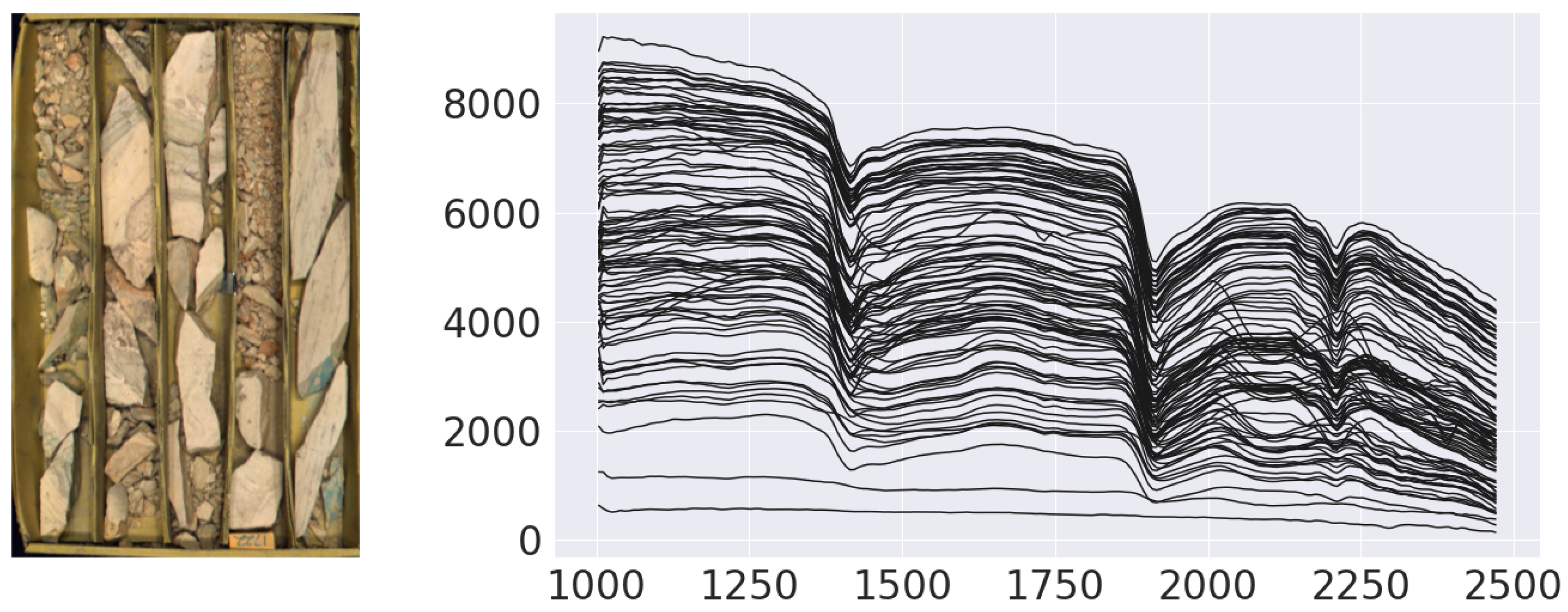
Masks are used to exclude data from the core boxes that are not useful to the mineral prediction network, such as the box frame, wooden blocks indicating the drill depth, and broken material that is too fine-grained to yield good reflectance or prohibits correct depth registration (see the left panel in Figure 2). This preprocessing masking step improves the overall quality of the data used to train the network and obtain the mineral predictions. The masks described in this section were later used in the mineral classification process described in Section 4.
TerraCore provided the data used to develop our neural networks, which included hyperspectral data together with manually-obtained masks for each of 118 core-boxes. Of these, 100 were randomly selected to train the CNN and the remaining 18 were used to check the quality of the masks.

3.1. Preprocessing

Training a CNN with SWIR images can be quite computationally expensive; for instance, a single SWIR image takes as much as 300 MB when represented as a multidimensional array. Thus, to develop a computationally and memory efficient CNN masking algorithm, we first performed a preprocessing dimensionality-reduction step. Principal component analysis (PCA) worked well for masking with this dataset. PCA is designed to determine a reduced set of orthogonal linear projections from a collection of variables to account for most of the sample variance (see, e.g., [10]). We found that the first three principal components accounted for 95–99% of the total sample variance across all core images, achieving a 100-fold size reduction of the arrays, which in turn led to a significant reduction in the total number of parameters required by the CNN model. Nevertheless, as storing the 100 SWIR images requires a large amount of memory, computing the standard singular value decomposition used in PCA remained challenging. Thus, we followed [11] and used an incremental version of PCA (implemented in scikit-learn) for the hyperspectral curve of each pixel. This approach computes the principal components by loading small batches into memory, then updating the estimates of the components. A final preprocessing step was to pad the resulting PCA images to ensure that a uniform size for easier use by the CNN.

3.2. Supervised Learning and Results

The uniformly-sized PCA images were combined with TerraCore masks to construct a complete dataset for training the masking model, and the same dataset was then used to perform supervised learning with a particular CNN image segmentation model, a simplified version of SegNet. The CNN SegNet architecture has been shown to be highly effective in image segmentation tasks [12]; it is a convolutional encoder–decoder model with a classification layer (see Figure 2 in [12] for an example). The encoder consists of thirteen convolution layers that are downsampled three times by a factor of two (as in the SegNet model) to a final size of 34 by 22 pixels. The decoder is composed of thirteen transposed convolution layers and is upsampled every three layers until the original image size is restored. This structure is able to capture low-resolution details in the image, although higher-resolution details may be lost and edges may be smoothed. To reduce this loss of high-resolution detail, SegNet employs skip connections that match encoder layers to decoder layers of the same size. These skip connections transfer information between layers by storing the indices of the pixels preserved during the downsampling stages, and fills the upsampled layers at those same indices (filling the rest by bilinear interpolation) to preserve the structure of the information in the image. We used a variation of this architecture that is straightforward to implement, simply passing the output of the layer before downsampling to the corresponding layer after upsampling, then adding these two outputs together. Using skip connections, SegNet is able to interpret images on scales ranging from single pixels to larger clusters of pixels that encode global information. Our model was trained using ADAM [13], a stochastic gradient-based method, which was run with a batch size of five images until the model stopped showing improvement (about 100 epochs).
The images from the final output were postprocessed using wavelet spatial smoothing with a second-order Daubechies wavelet (implemented in the package scikit-image [14]); here, by ‘order’ we mean the approximation order of the Daubechies wavelet (see [15]). The purpose of this postprocessing was two-fold: to produce masks that have continuous segments, and to remove artifacts that may have been introduced by the CNN SegNet model. Any neural network used is bound to make incorrect assignments that produce a noisy-looking mask; this is corrected by the smoothing step. It is analogous to drawing a mask by hand in that one tries to ignore small irregularities in favor of smoother segments of the core. As the net continues to learn with larger training sets, it makes fewer mistakes, requiring only small corrections or even no corrections at all. However, it should be noted that no smoothed data were used in the analysis described in Section 4; the smooth masks only provide the part of the data that to be used.
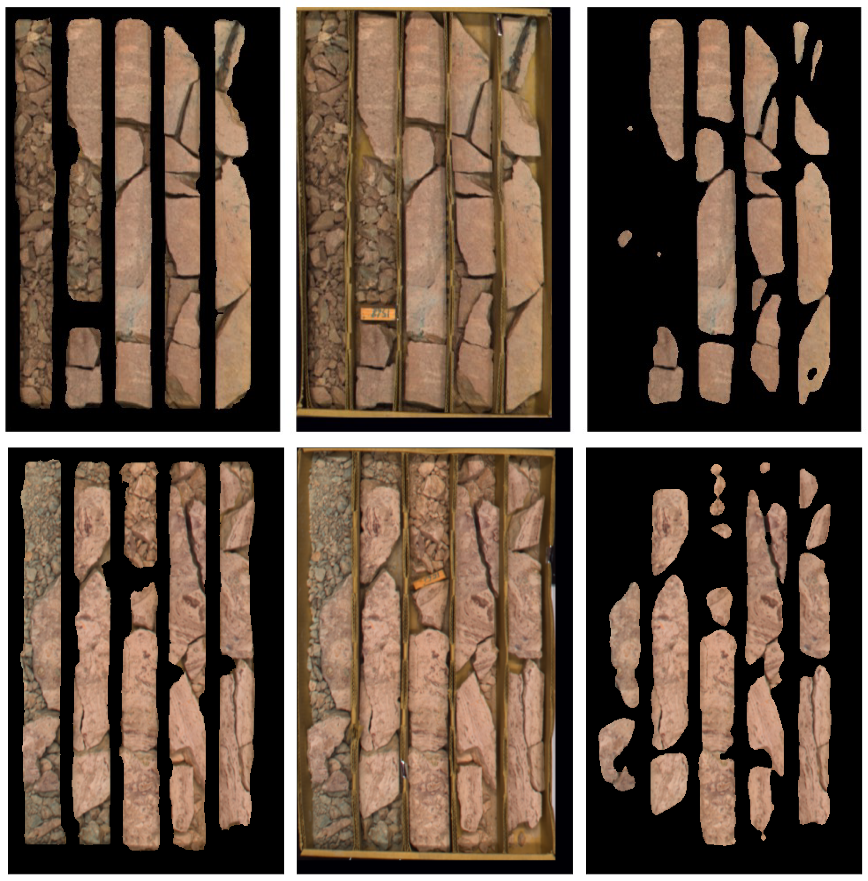
Higher-order wavelets were able to reproduce the original masks effectively; however, they failed to effectively remove the artifacts. We decided to use a second-order wavelet, as it provided the best combination of artifact removal, continuity, and mask quality. For example, the left panels in Figure 3 show the predicted filtered CNN masks of representative images of two drill cores in their core boxes (center). Note that a few rock fragments were removed, which is to be expected from any prediction network or algorithm trained on a limited sample. There is always a trade-off; the advantage of neural networks is that networks can learn, and keep improving the more they are trained.

3.3. Finer Masking

The masking procedure can be trained to identify and/or remove finer details such as broken material. For example, in certain applications it may be important to know where the broken material is located in the core boxes, as it does not properly represent the length of the drill core and may result in incorrect depth registration. In this case, it is possible to design the neural network to keep track of the location of the broken material. For this study, we simply masked these areas using an additional much smaller neural network that takes the masked output of the CNN and identifies pixels of interest while excluding broken material. This neural network consists of one fully connected layer with ReLU activation and a classification layer. The data for this model were generated based on eight randomly selected images. For each image, we used the K-means clustering method (see, e.g., [10]) to identify the pixels of interest by grouping all of the pixels into three clusters (‘core’, ‘background’, and ‘broken material’). We then determined the clusters containing pixels of interest by hand. Because the output of this model was somewhat noisy, a smoothing filter was applied to this secondary mask. Based on visual inspection, the filtered model was far more satisfactory and generalized well to the rest of the dataset. The right panels in each row in Figure 3 show the masks obtained after applying the finer masking procedure to two different core boxes. It can be seen that both masks effectively remove the background from this image and preserve the important sections of rock. The finer mask is much more selective and removes the broken material almost entirely, and even removes the cracks in between the larger rock pieces. It should be noted that the level of masking to be applied is user-defined, and depends on the particular application.

4. Modal Mineral Classification

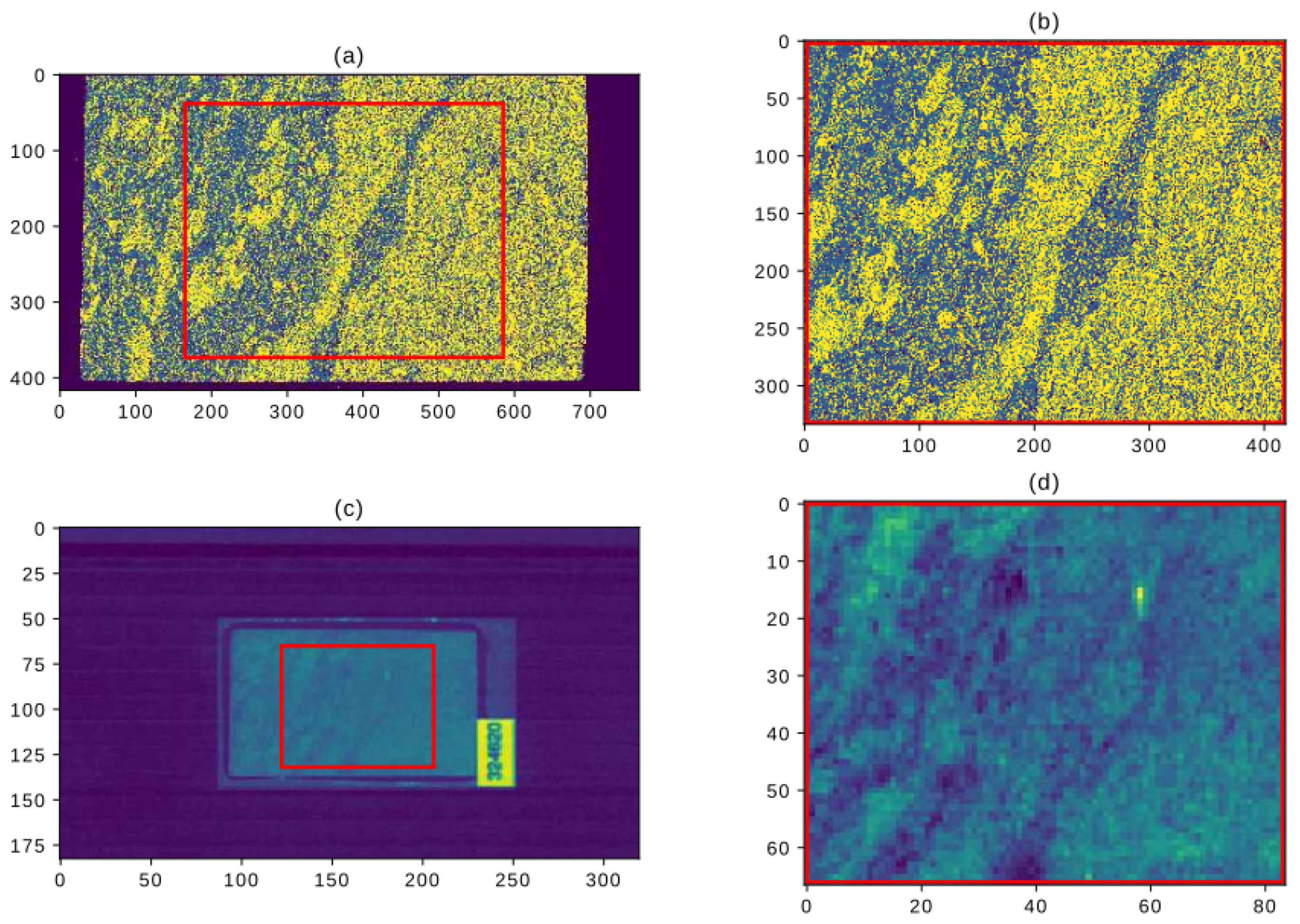
Following the masking procedure, we proceeded to make a mineral assignment for each pixel by identifying the most abundant mineral occurring in the pixel (i.e., modal abundance classification). This method is based on supervised learning. This time, thin sections scanned using SEM-based automated mineralogy were used as a reference to inform the SWIR spectroscopy data. An example of the training data is shown in Figure 4.
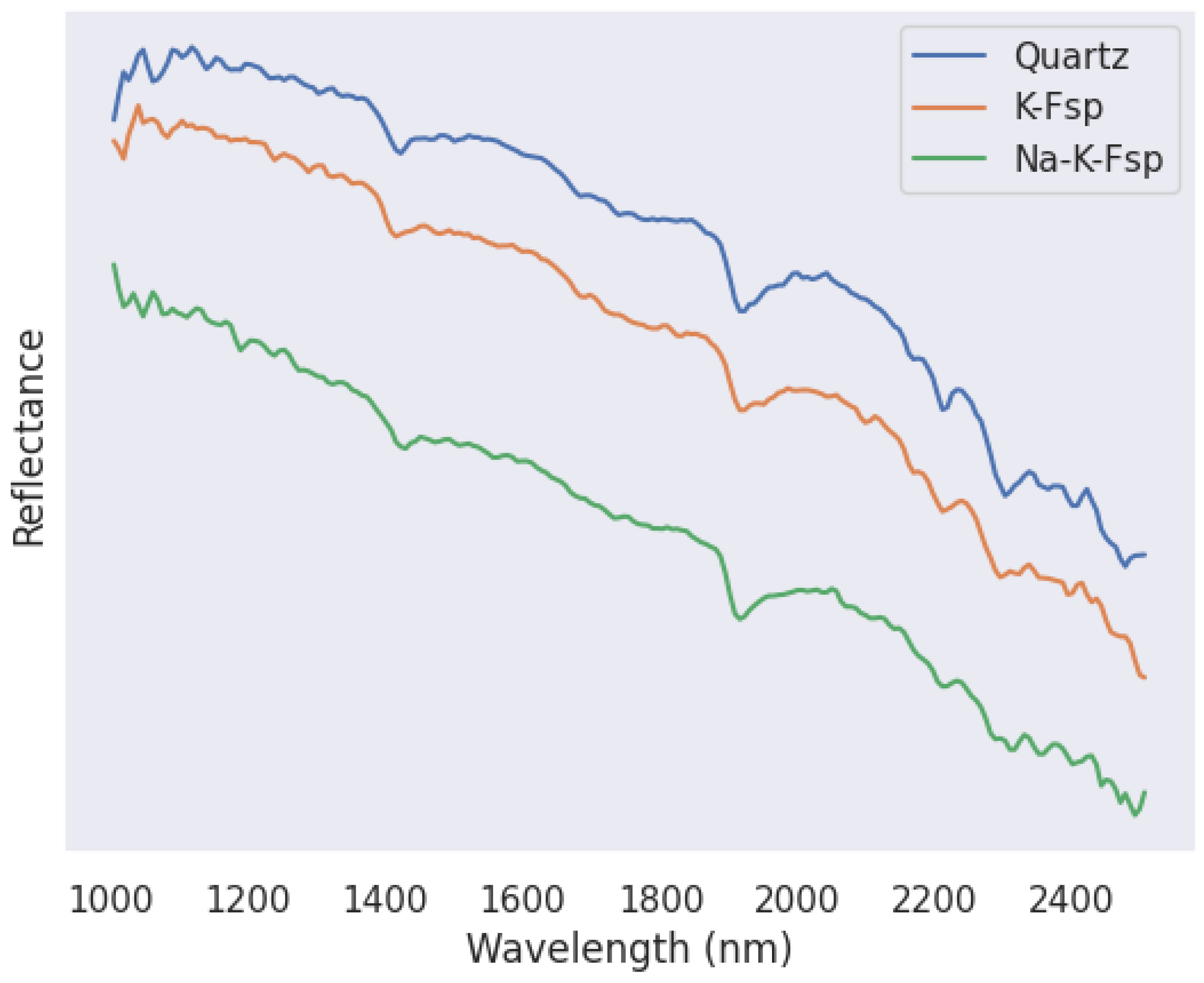
Unlike traditional spectral analyses, our classification model does not look for chosen characteristic features, which may not be known for certain minerals; instead, it learns identifying features from the entire spectral curve. As an illustration of how difficult it may be to distinguish minerals without identifying features, Figure 5 shows examples of three very similar reflectance curves, corresponding to quartz, K-feldspar, and Na-K-feldspar in the samples presented here.

4.1. Preprocessing

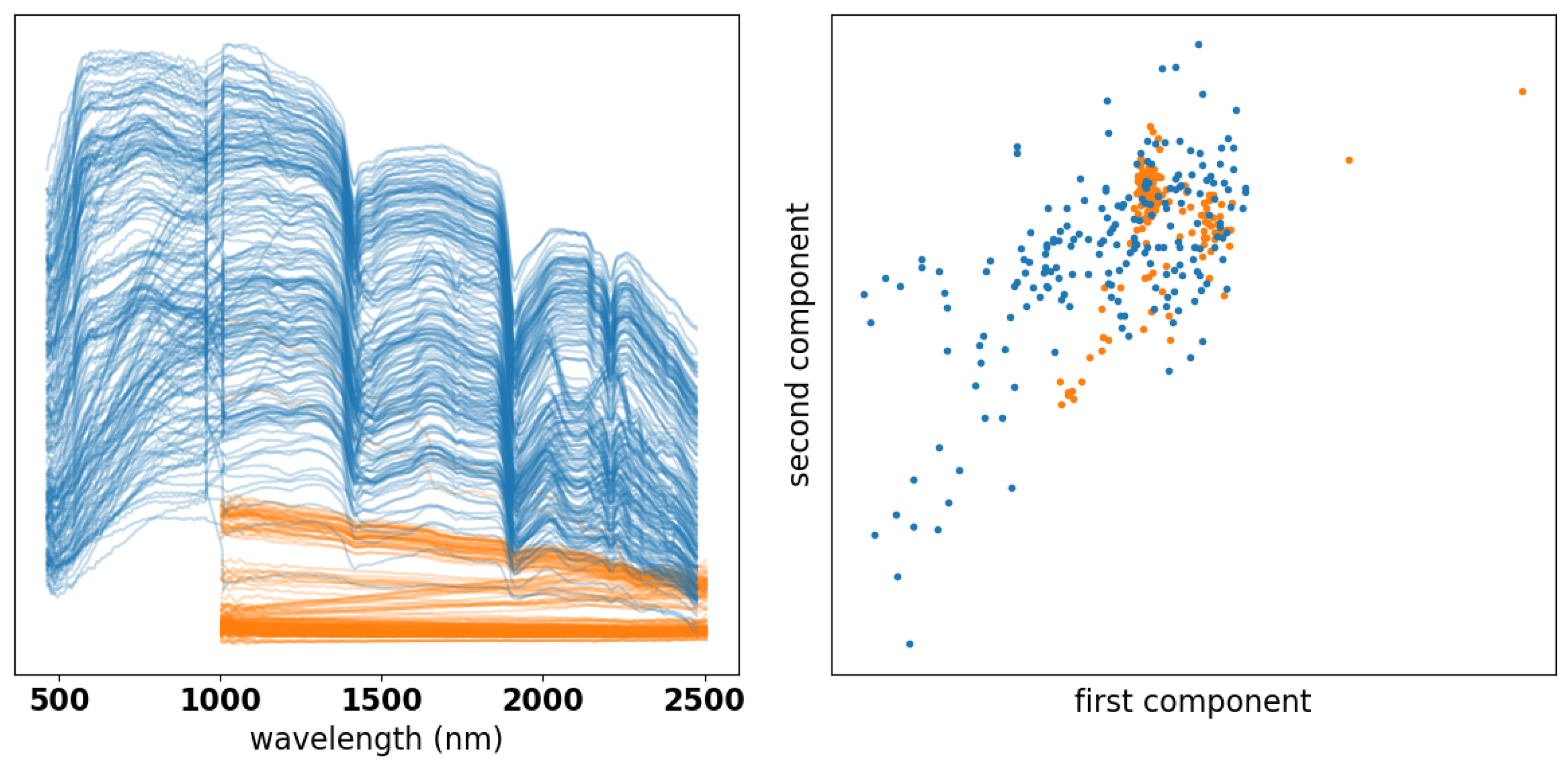
To learn identifying features, we first assisted the learning network by preprocessing the data to account for the fact that the thin section data and core box data differ in important ways which in themselves may not be useful for mineral identification. For instance, each thin section pixel is sampled uniformly at 214 wavelengths from 1004.05 nm to 2505.38 nm, and each pixel is 280 μm across. The thin section itself is approximately 60 μm thick, and was sampled behind a 1200 μm thick glass. On the other hand, each pixel in the core box consists of measurements at 411 wavelengths from 463.31 nm to 2476.54 nm, and each pixel is 1.2 mm across. The core box images are larger, and represent materials with widely varying scales and textures. These differences are quite apparent in the left panel of Figure 6, which displays core box data (blue) and thin section data (orange). This preprocessing step is more important with smaller amounts of data, as in our case; as more data become available, the network needs less help to learn identifying features, although dimensionality reduction techniques may be necessary to address computational cost.
We used a stochastic autoencoder model (SAE) to transform the data to a latent space where the two datasets have comparable distributions. Our SAE is a variation of the traditional variational autoencoder (VAE). VAEs are neural network models composed of an encoder that maps high-dimensional data to a low-dimensional latent space and a decoder that maps the latent space back to the original space [16,17]. The latent space is a set of pairs of vectors x ^ R p and s R p , s > 0 that define multivariate Gaussian distributions N ( x ^ , diag ( s ) ) . Variational autoencoders have been successfully used to simulate data by resampling from the learned distributions [16,17]; however, we used SAE as an alternative to PCA because the randomization tends to spread out distributions, which is desirable for our problem as we want to obtain a comparable distribution for the two data sources. More importantly, the SAE provided better classification results than training the same model and using PCA for dimensionality reduction, despite requiring more features to represent the data accurately.
We summarize the basic procedure before moving on to the details of our SAE. We started by linearly interpolating the core box data to 209 wavelengths, which was a subset of the thin section wavelengths in the range 1004.05–2470.37 nm (the maximum overlapping range between the two sampling intervals). The pixels in each dataset were centered and scaled to zero sample mean and unit variance for each wavelength. These two datasets were combined to train a linear SAE that learned a common distribution for the two data sources.
The model was trained by randomly sampling vectors from N ( x ^ , diag ( s ) ) and measuring the reconstruction error in R p . We used an embedding dimension p = 6 , as it was found to work best with our classification model. After the model was trained, the mean vector x ^ was used as the low p-dimensional representation of the data.
As mentioned above, our SAE is linear; that is, the encoder and decoders are linear functions of their input ( x ^ = Wx , x V T x ^ ), where W , V R p × 209 . The variance vector is defined as s = ( s i ) = exp ( S x + b ) with S R p × 209 and b R p , and the component-wise exponential function is used to ensure positive variances. The model parameters ( W , V , S , b ) are determined by minimizing the loss function ( x ; r ) :
( x ; r ) = x V T x ^ + diag ( s ) r 2 + τ i = 1 p 1 / s i ,
where r N ( 0 , I ) . Unlike the typical VAE model, which maximizes an evidence lower bound (as in [16,17]), our SAE model attempts to minimize the reconstruction error while penalizing small variance in order to mix the distributions in a common latent space. This loss is minimized using ADAM, where at each iteration and for each data point we randomly sampled r . The term with the τ parameter penalizes small variances, and τ controls the bias introduced by this penalty ( τ was chosen to be 10 4 based on experiments carried out on the data). We implemented this model using TensorFlow [18]. An example of the results is shown in the right panel of Figure 6, where the data from the left panel are shown in two of the six dimensions of the latent space.

4.2. Modal Learning

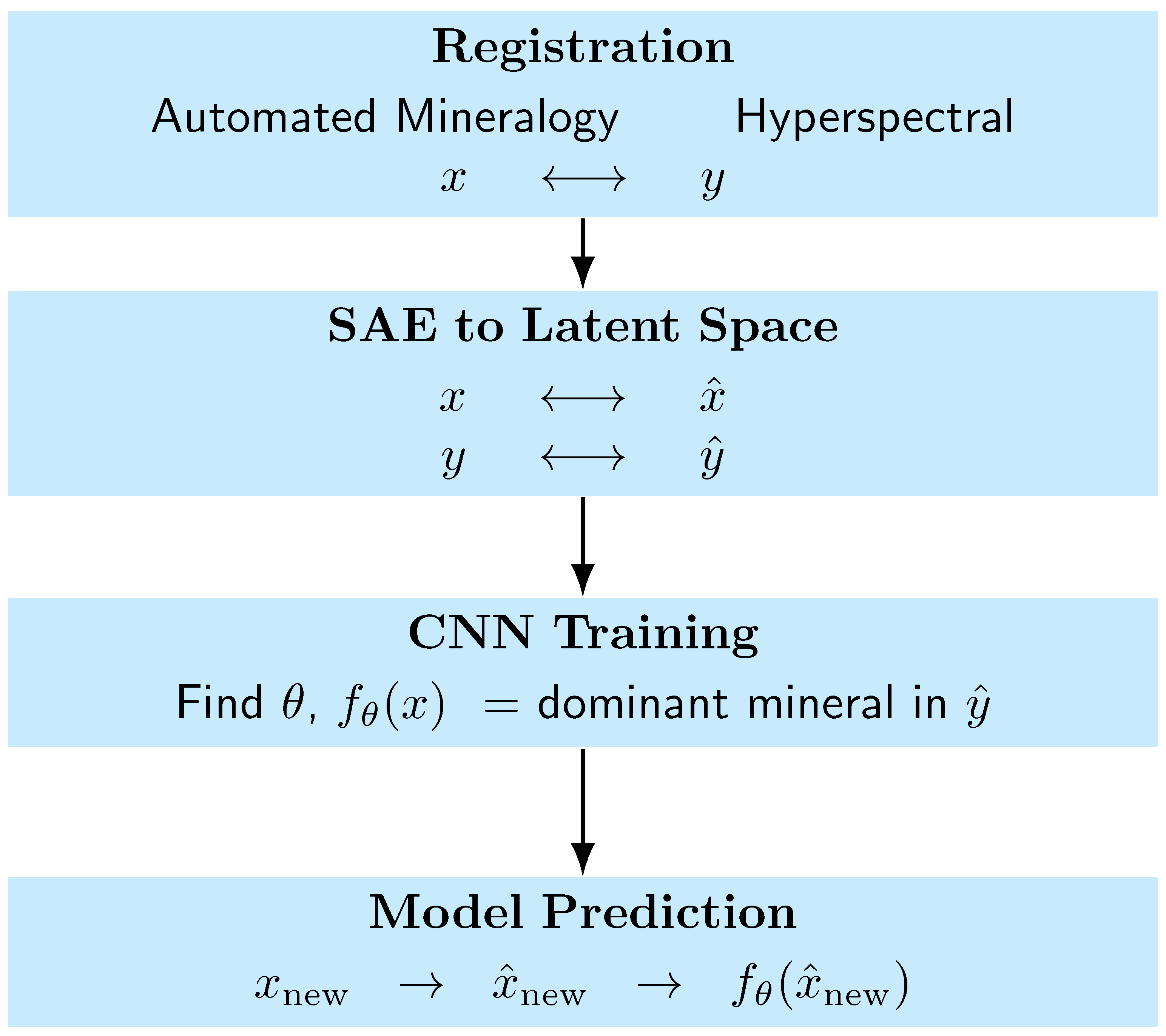
Our classification model uses the latent variable x ^ of a pixel (defined in Section 4.1) to predict a mineralogy label for such pixel. The model is a dense neural network implemented in the scikit-learn package [14]. The neural network has two hidden layers, the first with 100 neurons and the second with 50. Both layers used the ReLU activation function. The weights of each layer were obtained using penalized least squares, with the squared norm of the coefficients as the penalty. This is a standard approach used to regularize the minimization of a data misfit [19,20]. To reduce the correlation of neighboring pixels, all the pixels were stored in a large matrix and the entries were randomized. The training set consisted of 75% of the pixels, and the testing set consisted of the remaining 25%. These were used as training and testing sets for the entire modal prediction analysis. The optimal regularization parameter for the penalized least squares was determined using an exhaustive search to find the parameter that produced the best accuracy on the test set. We used GridSearchCV from the Scikit Learn Python package to perform this search [14]. Figure 7 provides a brief summary of the model identification procedure, from registration to prediction with new data.
The distribution of the minerals in the data is summarized in Table 1. Note that quartz and K-feldspar are the dominant minerals in the samples, while muscovite is the spectrally dominant mineral in the SWIR spectrum.

4.3. Results

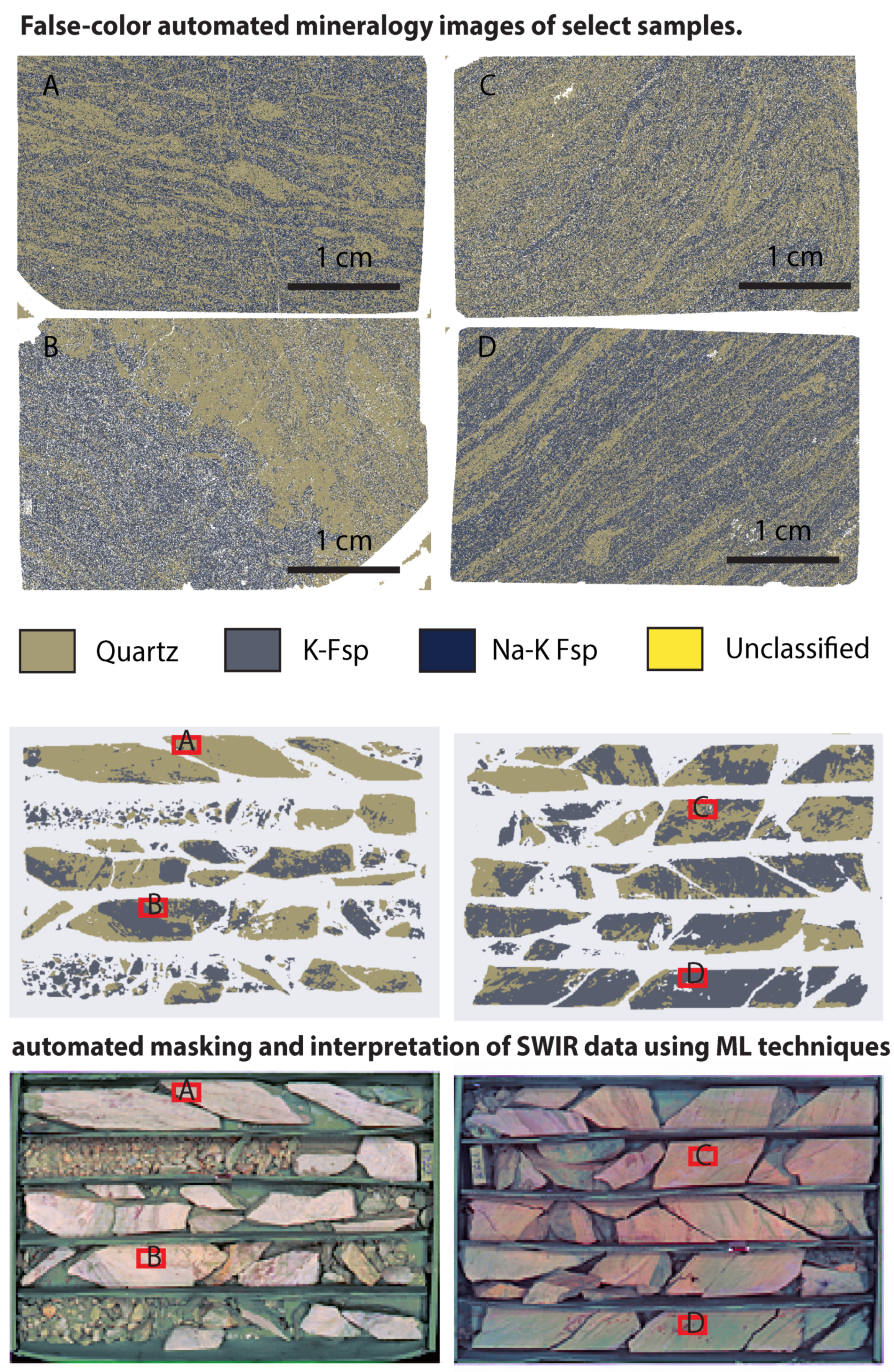
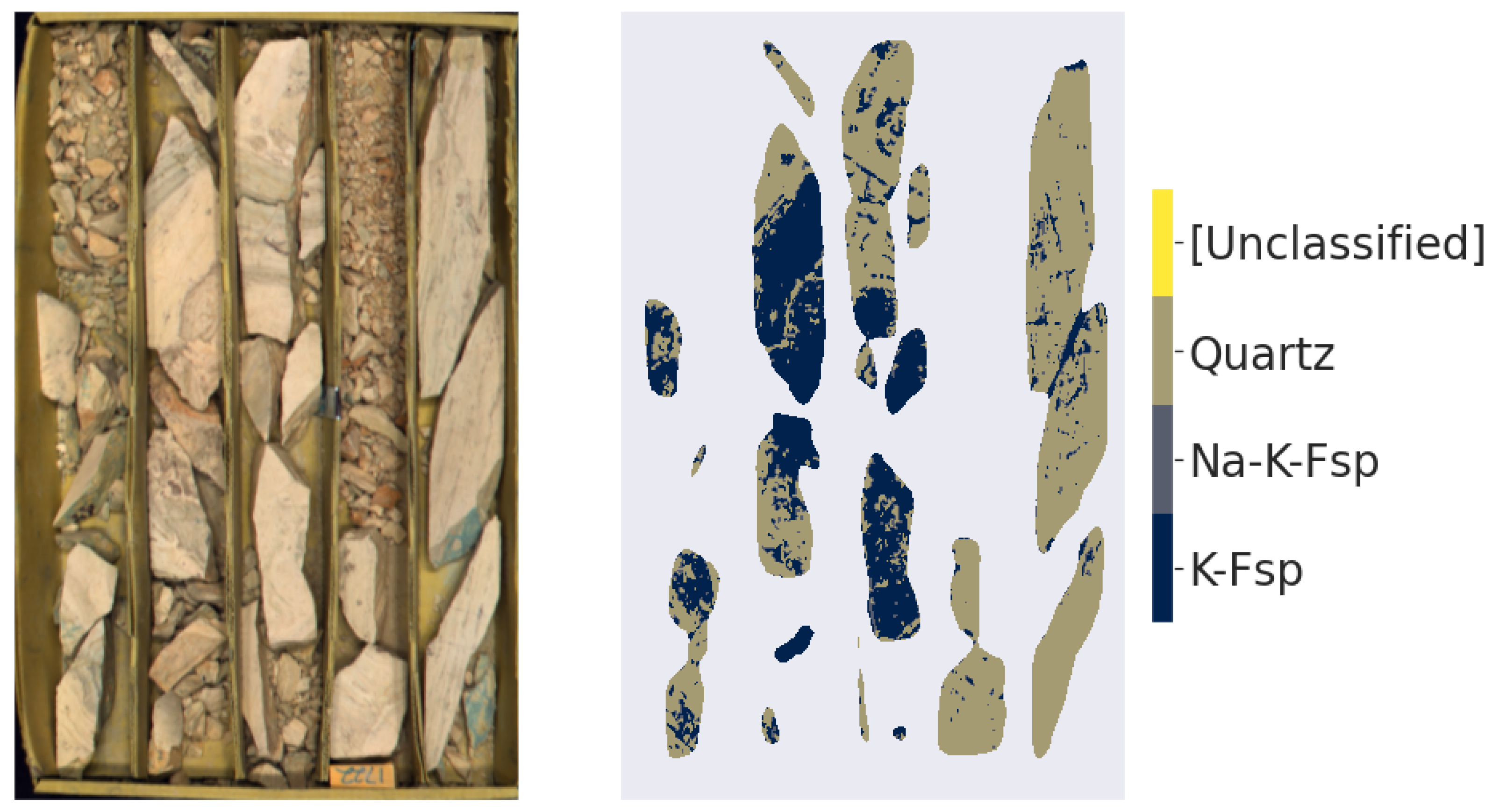
We applied SAE reduction to the pixels and predicted the mineralogy based on the latent variables, as explained in Section 4.1. Figure 8 and Figure 9 show predicted modal mineral abundance for two of the core box images. A first check of the results was qualitative based on the geology and mineralogy. Four of the thin sections analyzed using SEM-based automated mineralogy were sampled from the drill core boxes shown in Figure 5, which enabled us to visually verify the classification results; that is, the mineralogy, modal abundance, and textural information on core that were derived through machine learning were verified and compared to the outcomes of traditional core logging performed by trained geologists. Because both quartz and feldspar are invisible in traditional SWIR data interpretation, arriving at a correct identification while maintaining their respective spatial distributions shows the proposed methodology’s potential. As is evident in Figure 9, note that the secondary procedure described in Section 3 was used to remove broken material before applying the classification model.
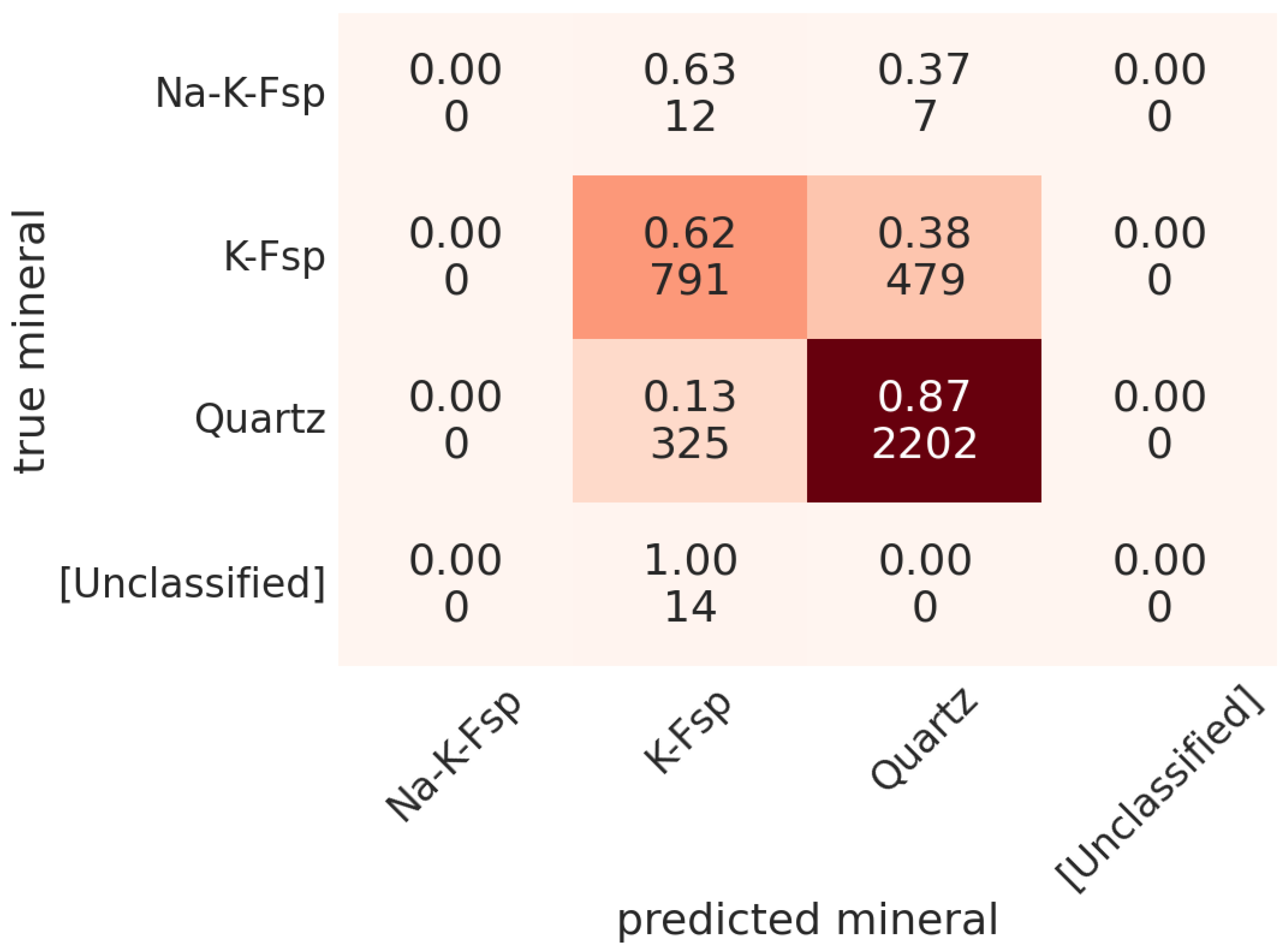
To evaluate the performance of the mineral predictions, the CNN was trained on a randomly selected set of 75% of the samples, while its predictions were tested on the remaining 25%. The accuracy was computed using the usual score, defined as the proportion of correct predictions in the test set. We obtained a prediction accuracy of 80%. For a second accuracy check, we used K-fold cross validation, which is a procedure used to test the accuracy of an algorithm by creating K training sets with non-overlapping test sets (see [10]). Using K = 10 , we averaged the results of our K-fold cross-validated accuracy scores and obtained an accuracy of 78%. This result is consistent with the first metric. Accuracy scores for individual minerals along with misclassification results are shown by the confusion matrix in Figure 10. For example, 62% of 791 K-feldspar pixels were correctly classified, and the rest were incorrectly classified as quartz.

4.4. Interpreting Accuracy

It is important to be careful when interpreting the reported accuracy results due to the large class imbalance in our data, which is evident in Table 1. It is well known that this type of class imbalance can result in predictions that may provide misleading results, as a classifier can simply predict the majority class and report an accuracy as high as the proportion of the majority class relative to all classes. Therefore, we used receiver operating characteristic (ROC) curves to test each of the classes as binary variables (see [21,22] for an introduction to ROC analysis). Because there were four classes in our data, we binarized our classes using a one-versus-rest scenario and computed the individual ROC curves for each of the four classes. In this one-versus-rest scenario, we treated one of the classes as the positive binary variable and combined the remaining three classes as the negative binary variable.
To generate the ROC curves, all of the predicted labels were arranged in an array with values corresponding to one of the four classes (we used the Yellowbrick Python package [23]). We then applied the one-versus-rest methodology described above to binarize each of the four classes. Next, each predicted label was scored based on the probability of the predicted class belonging to the actual class. This probability or score was computed from the classification decision rule determined by CNN. The instances (positive or negative classifications) were sorted by their scores, which were then compared to threshold values. The threshold values started at a very large value and decreased to zero. If a classifier output was above the threshold value, the classifier produced a positive classification outcome; otherwise, it produced a negative classification outcome. To aid in interpretation, in ROC space a threshold of infinity takes the point ( 0 , 0 ) , where no positive classifications are issued, and a threshold of zero takes the point ( 1 , 1 ) , where only positive classifications are issued. Intuitively, when the area under the ROC curve is close to one the classifier can be considered nearly perfect. Conversely, when the area under the curve is 0.5 or less it can be inferred that the classifier functionally behaves as random or worse, respectively. The ROC curves for each of the four mineral classes are shown in Figure 11. Because the ROC curves show performance that is strongly biased towards the true positive rate, it can be inferred that our algorithm is able to accurately predict modal mineral abundances despite the class imbalance.

4.5. Cluster-Wise Accuracy

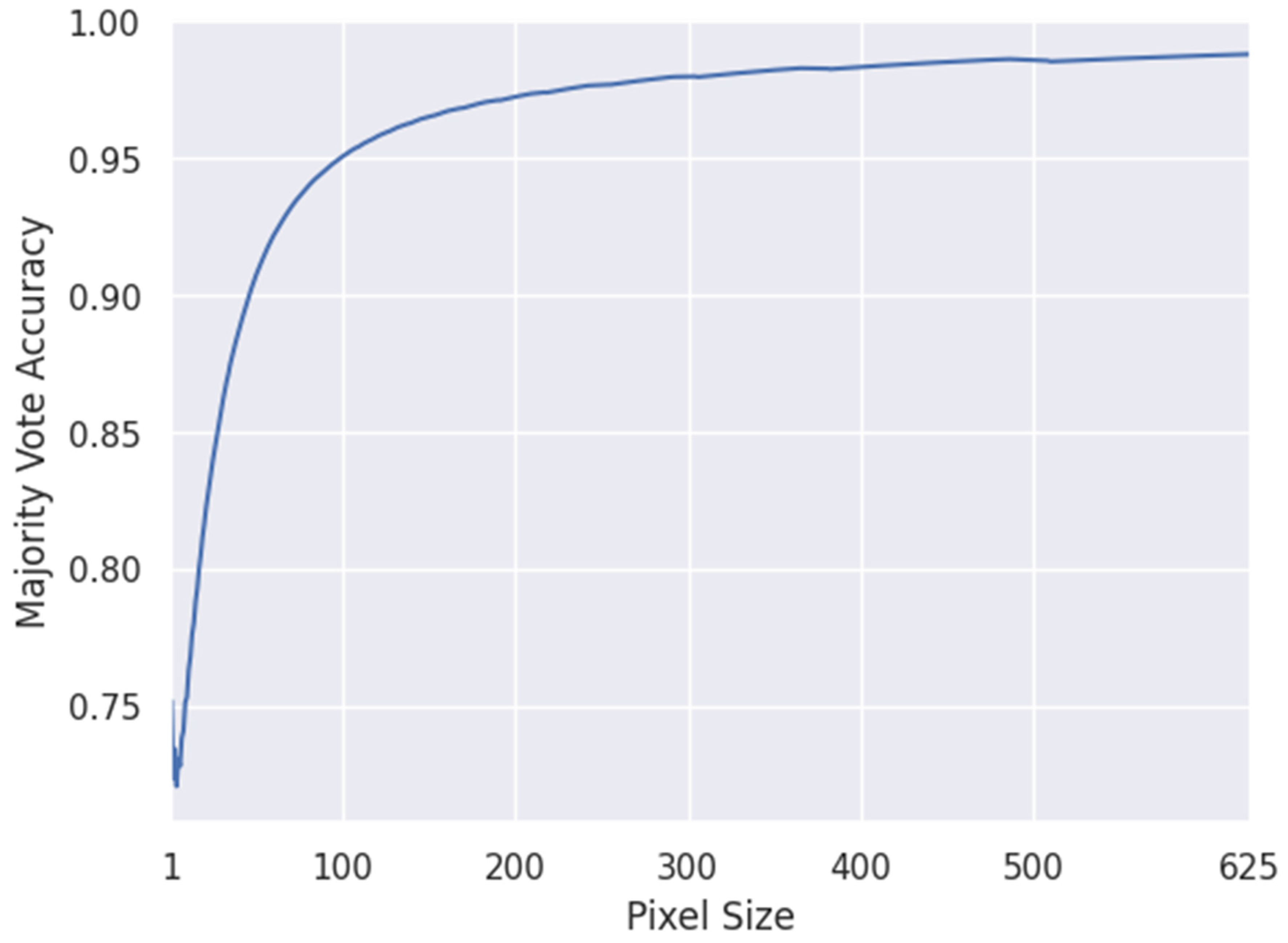
It is important to note that pixel-by-pixel prediction accuracy is often not as important to geologists as prediction of the mineral modal abundance in the textural domain. Furthermore, pixel-by-pixel accuracy is difficult to achieve because hyperspectral and SEM-based analytical results are sensitive to different material volumes within the sample. In addition, there may be small misalignments of measurements taken by different instruments. To assess how our mineral predictions perform with respect to small clusters, we again used K-fold cross validation, this time with majority-prediction votes on clusters of pixels across the sample. First, we split the hyperspectral test data and the ground truth automated mineralogy data into corresponding but non-overlapping square tiles of pixels. Starting with a single pixel, the tile size was increased by one pixel at a time until reaching tiles consisting of 25 × 25 pixels. We compared each hyperspectral test data tile to the associated automated mineralogy tile using a majority vote method; that is, we counted the number of pixels classified as a particular mineral and labeled the entire tile with the mineral that occurred the most in the tile. If two associated tiles had the same majority vote, we scored the match as a ‘1’; otherwise, it was scored as ‘0’. The proportion of matches out of the total number of tiles was recorded for each tile size. The results are shown in Figure 12, which shows a plot of the majority vote accuracy for each tile size (defined as the total number of pixels in the tile). As expected, for a single pixel the same 78% accuracy is recovered as was obtained before, while as the votes of more pixels are combined an accuracy above 90% is eventually reached. This can be interpreted as good accuracy for the prediction of the dominant mineral in small patches across the sample.

5. Summary and Conclusions

Hyperspectral SWIR data are widely used during various stages of a mine’s life cycle to complement traditional core logging. Hyperspectral core scanning is a rapid and non-destructive analytical method for mapping of minerals with diagnostic features, whereas SEM-based quantitative automated mineralogy can provide high-resolution mineralogical maps showing the mineral modal abundance of predominant minerals from select subsamples. The combination of rapid hyperspectral core scanning with quantitative mineralogical data derived from SEM-based automated mineralogy allows quantitative characterization of the mineralogy of drill core by upscaling SEM-based quantitative automated mineralogy information rather than mapping out spectrally dominant minerals. To develop this methodology, samples from the Castle Mountain low-sulfidation epithermal gold deposit in California were used. We produced mineralogy maps of drill core that were further evaluated to deduce mineral abundance data and textural information and used for comparison with core logs acquired through visual inspection. The proposed methodology for rapid mineralogical characterization can be easily applied to core from other deposits and deposit types. In addition to studies of ore deposits, this research has implications to the characterization of waste rock piles and tailings.
The use of SEM-based automated mineralogy data as training data for supervised machine learning was proposed and used previously by [3,4,24]. These studies demonstrated the potential of supervised machine learning to map the abundance of minerals with diagnostic features in wavelength spectra of interest using hyperspectral data. The method presented here focuses on mapping the predominant mineral rather than focusing on minerals with diagnostic features in the SWIR wavelength range (spectrally dominant minerals).
The methods presented here have the potential to enhance traditional techniques used in hyperspectral data interpretation of geological materials. We have shown that machine learning can be successfully used to interpret hyperspectral drill core data using a training dataset consisting of automated mineralogy and hyperspectral data collected from a small number of samples of the core to be analyzed. The proposed methodology was able to detect minerals that are undetectable by traditional hyperspectral data interpretation, overcoming previous limitations caused by the need to identify spectral features of minerals. The proposed methodology can reduce human bias in traditional visual core logging as well. In addition, the technique described in this paper illustrates how routine pre- and postprocessing tasks such as masking can be automated using machine learning techniques. Machine learning techniques were additionally used to address computational challenges in the implementation of the neural networks.
The present study shows that fusing SEM-based automated mineralogy data with hyperspectral data can be used to efficiently map both alteration mineralogy [3,4,24] and complete mineralogy, including minerals that are traditionally considered invisible in the SWIR wavelength spectrum. As a next step, image analysis could be applied to false color core maps of minerals to deduce information such as textural relationships, which could highlight characteristics such as flow ganding or automatically classify coherent felsic volcanic rocks and clastic volcanic rocks.
An important advantage of neural networks is that they can be used to obtain data-driven models of complex processes; however, their physical interpretation is typically difficult. For example, while our CNN model provided good mineral predictions we cannot easily say what spectral characteristics were useful to the network in reaching these identifications. We believe it is important to develop tools that can enable interpretation of the outcome of neural networks in order to determine what can be learned from them about rock physics and geology. This will be a part of our future work. For an introduction to the general problem of interpretating neural networks, see [25]. We intend to extend the proposed neural networks to estimate the percentage of different minerals in each pixel, not only the mode; this is a more difficult problem (known as unmixing) that requires larger training sets and is much more computationally demanding.

Author Contributions

Conceptualization, K.P. and T.M.; formal analysis, K.P., E.T. and T.M.; algorithm development, A.R. and A.V.; resources, K.P. and T.M.; data curation, A.R. and A.V.; writing—original draft preparation, A.V., A.R., K.P. and L.T.; writing—review and editing, L.T., M.C., E.T. and T.M.; funding acquisition, K.P. and T.M. All authors have read and agreed to the published version of the manuscript.

Funding

This work was supported in part by the National Science Foundation (NSF) and conducted within the Center to Advance the Science of Exploration to Reclamation in Mining (CASERM), which is a joint industry–university collaborative research center between the Colorado School of Mines and Virginia Tech under the NSF award numbers 1822146 and 1822108.

Data Availability Statement

All data used in this study are openly available at https://repository.mines.edu/, accessed on 30 April 2023.

Acknowledgments

TerraCore scanned and kindly provided data for this study. We are thankful to Todd Hoefen and Ray Kokaly from the U.S. Geological Survey for technical assistance and feedback, and to Kelsey Livingston, who was instrumental in sample preparation. Finally, we thank Gavriil Shchedrin and Samy Wu Fung for fruitful discussions on machine learning topics.

Conflicts of Interest

The authors declare no conflict of interest.

References

  1. Acosta, I.; Contreras, C.; Khodadadzadeh, M.; Tolosana-Delgado, R.; Gloaguen, R. Drill-core hyperspectral and geochemical data integration in a superpixel-based machine learning framework. IEEE J. Sel. Top. Appl. Earth Obs. Remote Sens. 2020, 13, 4214–4228. [Google Scholar] [CrossRef]
  2. Barton, I.F.; Gabriel, M.J.; Lyons-Baral, J.; Barton, M.D.; Duplessis, L.; Roberts, C. Extending geometallurgy to the mine scale with hyperspectral imaging: A pilot study using drone-and ground-based scanning. Mining Metall. Explor. 2021, 38, 799–818. [Google Scholar] [CrossRef]
  3. De La Rosa, R.; Khodadadzadeh, M.; Tusa, L.; Kirsch, M.; Gisbert, G.; Tornos, F.; Tolosana-Delgado, R.; Gloaguen, R. Mineral quantification at deposit scale using drill-core hyperspectral data: A case study in the Iberian Pyrite Belt. Ore Geol. Rev. 2021, 139, 104514. [Google Scholar] [CrossRef]
  4. Tusa, L.; Mahdi, K.; Contreras, C.; Rafiezadeh, K.; Fuchs, M.; Gloaguen, R.; Gutzmer, J. Drill-core mineral abundance estimation using hyperspectral and high-resolution mineralogical data. Remote Sens. 2020, 12, 1218. [Google Scholar] [CrossRef] [Green Version]
  5. Capps, R.; Moore, J. Castle Mountain Geology and Gold Mineralization, San Bernardino County, California and Clark County, Nevada; Nevada Bureau of Mines and Geology, Map 108; Department of Geology University of Georgia: Athens, GA, USA, 1997. [Google Scholar]
  6. Nielson, J.; Turner, R.; Bedford, D. Geologic Map of the Hart Peak Quadrangle, California and Nevada: A Digital Database; Technical Report, Open-File Report 99-34; U.S. Geological Survey: Reston, VA, USA, 1999.
  7. Secrest, G.; Tahija, L.; Black, E.; Rabb, T.; Nilsson, J.; Bartlett, R. Technical Report on the Castle Mountain Project Feasibility Study, San Bernardino County, California, USA; Technical Report, Feasibility Study for Equinox Gold; 2021; 453p. Available online: https://www.sec.gov/Archives/edgar/data/1756607/000127956921000353/ex991.htm (accessed on 14 June 2023).
  8. Smith, G.M.; Milton, E.J. The use of the empirical line method to calibrate remotely sensed data to reflectance. Int. J. Remote Sens. 1999, 20, 2653–2662. [Google Scholar] [CrossRef]
  9. Bedell, R.; Coolbaugh, M. Atmospheric corrections. Rev. Econ. Geol. 2009, 16, 257–263. [Google Scholar]
  10. Johnson, R.A.; Wichern, D.W. Applied Multivariate Statistical Analysis, 6th ed.; Pearson: London, UK, 2007. [Google Scholar]
  11. Ross, D.A.; Lim, J.; Lin, R.; Yang, M. Incremental learning for robust visual tracking. Int. J. Comput. Vis. 2008, 77, 125–141. [Google Scholar] [CrossRef]
  12. Badrinarayanan, V.; Kendall, A.; Cipolla, R. SegNet: A deep donvolutional encoder-decoder architecture for image segmentation. IEEE Trans. Pattern Anal. Mach. Intell. 2017, 39, 2481–2495. [Google Scholar] [CrossRef] [PubMed]
  13. Kingma, D.P.; Ba, J. ADAM: A method for stochastic optimization. arXiv 2017, arXiv:cs.LG/1412.6980. [Google Scholar]
  14. Pedregosa, F.; Varoquaux, G.; Gramfort, A.; Michel, V.; Thirion, B.; Grisel, O.; Blondel, M.; Prettenhofer, P.; Weiss, R.; Dubourg, V.; et al. Scikit-learn: Machine learning in Python. J. Mach. Learn. Res. 2011, 12, 2825–2830. [Google Scholar]
  15. Daubechies, I. Society for Industrial and Applied Mathematics. Ten Lect. Wavelets 1992. [Google Scholar]
  16. Kingma, D.P.; Welling, M. An introduction to variational autoencoders. Found. Trends Mach. Learn. 2019, 12, 307–392. [Google Scholar] [CrossRef] [Green Version]
  17. Murphy, K.P. Probabilistic Machine Learning: Advanced Topics; MIT Press: Cambridge, MA, USA, 2023. [Google Scholar]
  18. Abadi, M.; Agarwal, A.; Barham, P.; Brevdo, E.; Chen, Z.; Citro, C.; Corrado, G.S.; Davis, A.; Dean, J.; Devin, M.; et al. TensorFlow: Aarge-scale machine learning on heterogeneous systems. arXiv 2015, arXiv:1603.04467. [Google Scholar]
  19. Green, P.J.; Silverman, B.W. Nonparametric Regression and Generalized Linear Models: A Roughness Penalty Approach; Chapman & Hall: Boca Raton, FL, USA, 1993. [Google Scholar]
  20. Tenorio, L. An Introduction to Data Analysis and Uncertainty Quantification for Inverse Problems; Society for Industrial and Applied Mathematics; SIAM: Philadelphia, PA, USA, 2017. [Google Scholar]
  21. Fawcett, T. An introduction to ROC analysis. Pattern Recognit. Lett. 2006, 27, 861–874. [Google Scholar] [CrossRef]
  22. Provost, F.; Fawcett, T. Analysis and visualization of classifier performance with nonuniform class and cost distributions. In AAAI-97 Workshop on AI Approaches to Fraud Detection and Risk Management; The AAAI Press: Menlo Park, CA, USA, 1997; pp. 57–63. [Google Scholar]
  23. Bengfort, B.; Bilbro, R.; Danielsen, N.; Gray, L.; McIntyre, K.; Roman, P.; Poh, Z. Yellowbrick. Version 0.9.1. Available online: http://www.scikit-yb.org/en/latest/ (accessed on 30 April 2023).
  24. Acosta, I.C.C.; Khodadadzadeh, M.; Tusa, L.; Ghamisi, P.; Gloaguen, R. A machine learning framework for drill-core mineral mapping using hyperspectral and high-resolution mineralogical data fusion. IEEE J. Sel. Top. Appl. Earth Obs. Remote Sens. 2019, 12, 4829–4842. [Google Scholar] [CrossRef]
  25. Montavon, G.; Samek, W.; Müller, K.R. Methods for interpreting and understanding deep neural networks. Digit. Signal Process. 2018, 73, 1–15. [Google Scholar] [CrossRef]
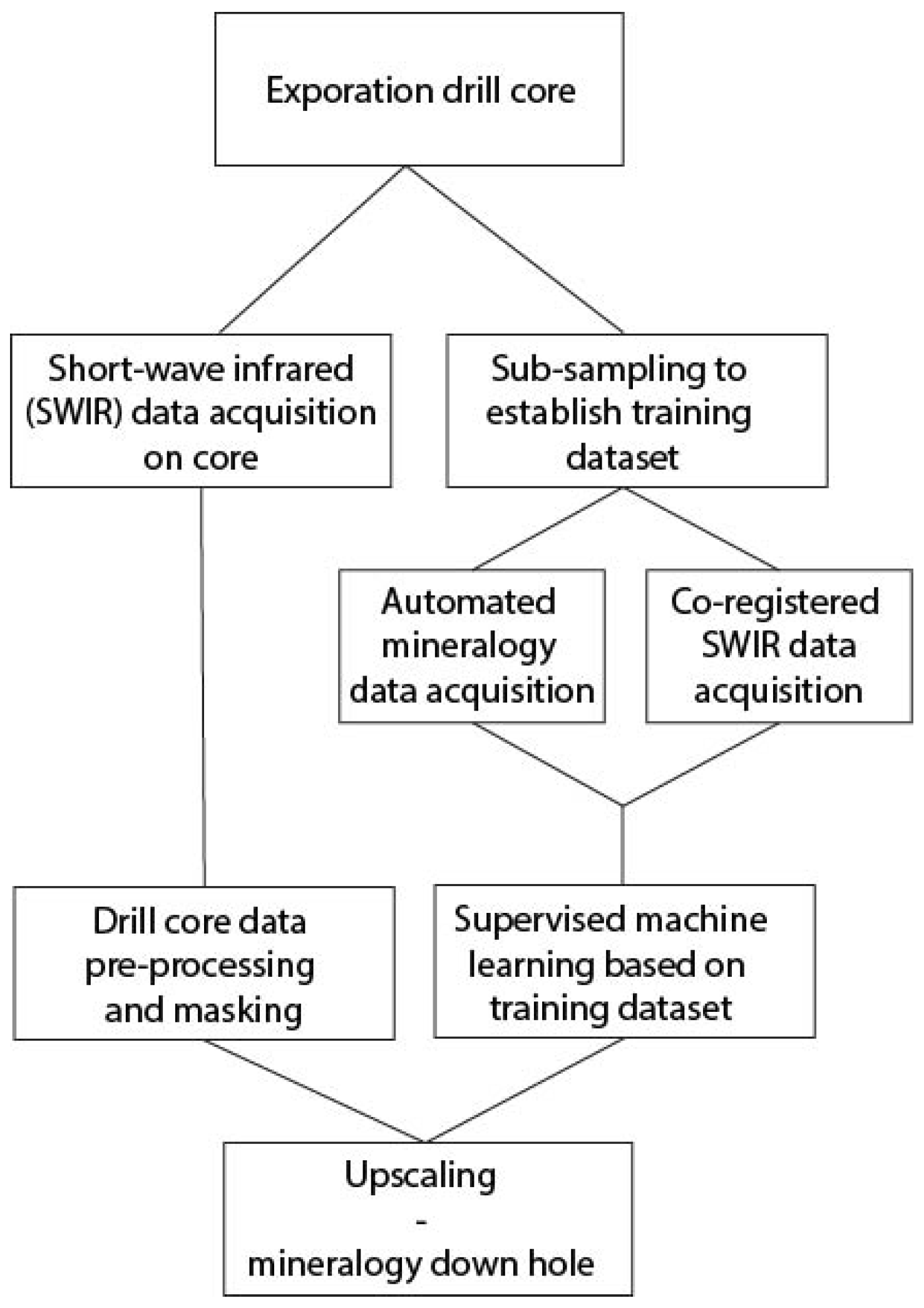
Figure 1. Flowchart of data acquisition and interpretation using machine learning algorithms.
Geosciences 13 00192 g001
Figure 2. Example of core box (left) with associated SWIR spectra (right); see Figures 6 and 9 for further discussion.
Geosciences 13 00192 g002
Figure 3. Masks obtained with the method described in Section 3. Each row shows a core box (middle), a neural network-generated mask (left), and a finer mask (right) that removes broken material.
Geosciences 13 00192 g003
Figure 4. Automated mineralogy data (top) with predominant minerals highlighted in yellow (quartz) and blue (K-feldspar) paired with associated spectral data (bottom). The sample includes muscovite as well, which is not abundant enough to be the predominant mineral in any of the pixels. The two images on the right hand-side were used to train the mineral identification network. The field of view in (a,c) is 30 mm, whereas the field of view in (b,d) is 17 mm.
Geosciences 13 00192 g004
Figure 5. Examples of absorbance curves from thin section data for quartz, K-feldspar, and Na-K-feldspar. While these absorbance curves look virtually identical to the naked eye, as they lack diagnostic features, the machine learning algorithm is able to use all the curves to learn subtle differences that can be used to correctly identify different minerals.
Geosciences 13 00192 g005
Figure 6. The left panel shows a sample of the absorbance curves from the core box data (blue) and thin section data (orange). It can be seen that the spectrally dominant mineral is muscovite, as indicated by the 2200 nm feature. Broad absorption features in the VNIR spectrum range indicate Fe2+, Fe3+, or a combination of the two. The right panel shows the same data in the first two components of x ^ (as defined in Section 4.1) for the same sample.
Geosciences 13 00192 g006
Figure 7. Flowchart summarizing the machine learning algorithm from registration to prediction at the drill core scale.
Geosciences 13 00192 g007
Figure 8. Graphical summary of the modal mineral classification procedure. The first two rows at the top show the automated mineralogy data of four thin sections (with legend). The origin of these thin sections is indicated in red in the drill core images show at the bottom (the bottom two rows). The mineralogical drill core predictions are shown in the third row with the same false color coding as the automated mineralogy images (the top two rows).
Geosciences 13 00192 g008
Figure 9. A core box and its predicted modal mineral abundances.
Geosciences 13 00192 g009
Figure 10. Confusion matrix of modal mineral abundances predicted in one of the thin sections.
Geosciences 13 00192 g010
Figure 11. ROC curves for each of the four classes against all the others. The curves summarize the classification performance by plotting the false positive rates against the true positive rates.
Geosciences 13 00192 g011
Figure 12. K-fold cross-validation estimate of the majority vote accuracy as a function of tile size.
Geosciences 13 00192 g012
Table 1. Number of training and test samples (pixels) used for each mineral.
ModelTraining SamplesTest Samples
Quartz76162538
K-Feldspar37851263
Na-K-Feldspar6412
Unclassified5417
Disclaimer/Publisher’s Note: The statements, opinions and data contained in all publications are solely those of the individual author(s) and contributor(s) and not of MDPI and/or the editor(s). MDPI and/or the editor(s) disclaim responsibility for any injury to people or property resulting from any ideas, methods, instructions or products referred to in the content.