Article

The Influence of Input Motion Scaling Strategies on Nonlinear Ground Response Analyses of Soft Soil Deposits

1
Faculty of Engineering and Architecture, Department of Civil Engineering, Necmettin Erbakan University, Konya 42090, Turkey
2
Department of Civil, Environmental, Land, Building Engineering and Chemistry (DICATECh), Politecnico di Bari, via Orabona 4, 70125 Bari, Italy
3
School of Engineering, Newcastle University, Newcastle upon Tyne NE1 7RU, UK
*
Author to whom correspondence should be addressed.
Geosciences 2023, 13(1), 17; https://doi.org/10.3390/geosciences13010017
Submission received: 23 November 2022 / Revised: 28 December 2022 / Accepted: 5 January 2023 / Published: 6 January 2023

Abstract

:
A key issue for the estimation of ground shaking is the proper selection of input motions at the seismic bedrock. At the same time, the effect of the input motion scaling strategy on structural response is typically studied disregarding the presence of the soil deposit. In this work, different soft soil deposits are selected by varying the shear wave velocity profiles and the depth to the seismic bedrock, modelling the soil behaviour through a nonlinear constitutive model implemented into a fully coupled FE code. Seven input motions are retrieved for several selection strategies in conjunction with two seismic intensity levels. Hence, more than 300 one-dimensional ground response analyses are performed. The results of the analysed cases, which are presented in terms of spectral response at ground surface and amplification factors, indicate that: (i) the use of an advanced elasto-plastic soil constitutive model accounts for nonlinear ground response effects, including higher site amplification in the mid-period range and deamplification of the peak ground accelerations; (ii) the different scaling strategies lead to comparable mean values of the amplification factors, and (iii) the variability of the amplification factors is significantly reduced when the scaling strategy seeks the compatibility with the target spectrum over a specified period range. The research will aid the prediction of local seismic site response over large areas, particularly in the absence of the fundamental period of a structure and facilitate its use in general recommendation for quantifying and reducing uncertainty.

1. Introduction

The alteration of earthquake characteristics from the seismic bedrock to the ground surface, due to local site conditions, is of great interest for the engineering community dealing with the seismic design of earth structures, buildings, and infrastructure [1]. A realistic prediction of ground response in soft soil deposits is particularly important since seismic wave propagation can be considerably affected by the material nonlinearities. The common method of predicting local site effects is to propagate seismic input motions through horizontally layered soil deposits using simple or advanced numerical methods. This enables the assessment of the surface acceleration time histories, response spectra, amplification factors (AFs, the ratio of free-field and input motions integral quantities), soil stiffness degradation, and associated hysteretic dissipation in response to shear strains induced by a possible earthquake event [2,3].
Ground response analyses, known also as local seismic site response (LSSR) analyses, are mainly governed by the bedrock input motion, the nonlinear dynamic features of the soil deposit, and its initial shear wave velocity profile. These components involve some uncertainties attributed to: (i) the ambiguity in the selection of a credible earthquake event with specific features from a database (i.e., magnitude, distance from the fault, fault mechanism, and target response spectrum compatibility) [4], (ii) the aleatory uncertainty in the definition of the shear wave velocity profile due to the heterogeneity of the site geology [5,6,7], and (iii) the epistemic uncertainty affecting laboratory and in-situ tests used to determine the material nonlinear dynamic properties [8,9]. These uncertainties may ultimately cause bias in site response predictions if they are not properly accounted for in the analysis [5].
Research has been directed to the above uncertainties to quantify their possible effects on ground response predictions. For this purpose, Monte Carlo simulations have been conducted with linear or nonlinear soil models by varying site properties [10,11,12,13]. While these studies explicitly indicate the importance of accounting for the shear wave velocity, stiffness degradation, and damping ratio variability in LSSR analyses, they also recognise the fundamental impact of bedrock motion characteristics on the statistical stability of the results. To minimize the bias in ground response predictions, and, thus, the number of simulations to be performed, the input motions, selected from available databases, can be subjected to some modification/scaling. Different input motion scaling methods, such as the peak ground acceleration (PGA) scaling, spectral matching, and the mean squared error approach, have been proposed, mainly in structural engineering literature [14,15,16,17,18], but their application to geotechnical earthquake engineering problems is limited [19,20,21,22,23]. At the same time, the compatibility of scaled motions is sought with respect to a target response spectrum provided by national and international codes [15]. For soft soils, this can be obtained from the statistical analysis of very few real earthquake recordings [24,25]. Moreover, no recommendations are provided by technical codes with reference to the selection/scaling strategies to be adopted with the aim of predicting ground motion modifications at surface over large areas. In fact, different types of structures and infrastructure (i.e., different natural periods of vibration) should be considered in this case and, consequently, the selection of input motions for LSSR analyses is a non-trivial task. For instance, guidelines have been proposed by the Italian Department of Civil Protection to perform seismic microzonation studies at the scale of the urban area [26]. In this context, Falcone and co-workers [27,28] performed site response analyses over the entire territory of Italy, excluding Sardinia region, based on Random Vibration Theory, but using response spectra as input motions. Therefore, codified procedures for selecting accelerograms over large areas still need to be provided.
This paper investigates the influence of different earthquake scaling strategies on the free-field ground response of ideal soft soil deposits. Four input motion scaling approaches are used: (1) scaling at PGA only, (2) scaling at the natural period of a soil column (T1), (3) scaling in a period range of 0.2T1–2T1 according to EC8 [15], and (4) matching the spectral shape of the input response spectrum to the target demand using the spectral matching method. Sets of seven bedrock motions are used for each scaling strategy, considering two seismic intensity levels of 0.15 g and 0.35 g representative of weak and strong earthquake events, respectively. Advanced time-domain analyses are conducted using an elasto-plastic effective stress-based constitutive model, capable of accurately capturing the effects of soil nonlinearity during dynamic loading. The results of the numerical simulations are interpreted in terms of spectral response at ground surface and AFs. The effect of the deposit thickness on the AFs is also considered. Throughout the paper, the comparison with EC8 prescriptions is presented to evaluate the performance of the scaling procedures with reference to the seismic response of soft soil deposits and to provide recommendations for researchers interested in LSSR analyses conducted over large areas.

2. Materials and Numerical Models

The ground response of ideal soft clay deposits is modelled by means of nonlinear finite element (FE) simulations carried out within the fully coupled program SWANDYNE II [29], in which the u–p formulation (where u is the displacement and p is the pore pressure) is implemented to solve solid-fluid interaction under dynamic conditions [30,31]. The FE code has been successfully validated against the equivalent linear solution for the one-dimensional propagation of shear waves in viscoelastic deposits [3]. In the nonlinear FE analyses, the Rouainia and Muir Wood (RMW) advanced soil constitutive model [32] is adopted to simulate the clay behaviour during the seismic excitation. The RMW constitutive model is implemented in SWANDYNE II using an explicit stress integration scheme. RMW has been successfully employed to predict the dynamic performance of different earth structures [33,34,35]. It has been shown to accurately reproduce the decay of shear stiffness with strain amplitude, the corresponding increase of hysteretic damping, the related accumulation of excess pore water pressure, and structure degradation of clays in undrained conditions [36]. The RMW model parameters are determined by simulating a series of undrained cyclic simple shear tests under controlled strain levels in order to obtain the normalised shear modulus, GS(γ)/G0, and damping curves, D(γ), predicted by the model for two soft soil materials: Avezzano clay [37] (central Italy) and Champlain clay [38] (Eastern Canada). Champlain clay is characterised by an open structure due to a rapid sedimentation [39,40] coupled with the high salinity of the depositional environment. These factors have led to a very high natural water content, high sensitivity, low shear strength, and high compressibility. A typical soil profile consists of topsoil, weathered clay crust, soft silty clay of marine origin, very soft clayey silt, and a deep layer of dense sand [41]. The Avezzano site is situated in the Fucino basin, a large intra-mountain depression located 80 km east of Rome and surrounded by the Apennines mountains. The basin originated from the sedimentation of fluvio-lacustrine sediments during the Pleistocene period and is composed by top layers of clayey and silty soils, with sand and gravel found underneath. The deposit is geologically normally consolidated, and the silty clay layers are characterised by a very low plasticity and high values of calcium carbonate content [42].
The calibrated model parameters and the corresponding nonlinear curves obtained with RMW are reported in Table 1 and Figure 1, respectively. It should be noted that the predictions obtained with the advanced constitutive model are in good agreement with the laboratory data for both clays and fall within the expected range by Darendeli [37]. In the dynamic simulations conducted within SWANDYNE II, only 2% Rayleigh damping [43,44,45] is added to avoid the propagation of spurious high frequencies and to compensate for the RMW underestimation of damping in the small-strain range [46].
Figure 2a shows the shear wave velocity profiles, VS1 and VS2, for Avezzano and Champlain clays, respectively. Such VS profiles are associated with the initial stiffness profile of the deposit obtained using Equation (1), proposed by Viggiani and Atkinson [47], for the dependency of the small-strain shear modulus G0 on the mean effective stress and overconsolidation ratio:
G 0 p r = A p p r n R 0 m
where A, m, and n are dimensionless stiffness parameters, which depend on PI, p’ is the effective mean stress, p’r is the reference pressure equal to 1 kPa, and R0 is the overconsolidation ratio. In particular, A, m, and n are set equal to 2915, 0.22, and 0.78, respectively, for the Avezzano clay and correspond to a PI equal to 10%; they are set equal to 1400, 0.22, and 0.76 for the Champlain clay, consistently with a PI of 22%. The overconsolidation ratio over a depth of 50 m is assumed, on average, equal to 1.2 for the Avezzano deposit and 2.1 for the Champlain clay, as indicated by the corresponding laboratory data. The Champlain deposit is characterised by a VS equal to 280 m/s at 50 m below ground surface (b.g.s.), while the Avezzano clay is slightly stiffer, reaching a VS of about 400 m/s at the same depth. It should be noted that the EC8 soil class depends mainly on the mean shear wave velocity in the upper 30 m, VS30, with the exception of soil class E, for which VS30 is lower than 360 m/s, and for a seismic bedrock depth, Hdeposit, in the range of 5 to 20 m. Accordingly, both Champlain and Avezzano clay deposits should be considered as EC8 class E for Hdeposit = 15 m (Figure 2b). Moreover, the Avezzano deposit can be classified as class C for Hdeposit equal to 30 m and 50 m (Figure 2c,d), while the Champlain deposit is classified as class D for Hdeposit equal to 30 m and 50 m (Figure 2c,d). Considering the Avezzano deposit, VS30 is 378 m/s for a 15 m column and 282 m/s for Hdeposit deeper than 30 m, while for the Champlain clay, VS30 is equal to 234 m/s and 166 m/s at the same depths. It is worth mentioning that EC8 class B is defined by VS30 in the range of 360 to 800 m/s for deposits at least several tens of meters in thickness. Therefore, the case of VS30 equal to 378 m/s and Hdeposit = 15 m is considered to represent a soil of class E rather than class B.
Figure 1. Shear modulus degradation and damping curves predicted by the RMW model for Avezzano and Champlain clays, compared to laboratory data [37,38] and curves by Darendeli [48].
Geosciences 13 00017 g001
The numerical models consist of 5 m wide columns with variable depths (i.e., 15, 30, and 50 m), discretised with 250, 1 × 1 m isoparametric quadrilateral finite elements, with 8 solid nodes and 4 fluid nodes to ensure that the seismic wave transmission is represented accurately through the FE mesh. The water table is assumed at ground surface, while the total unit weight of the soil is set equal to 18 kN/m3 for both the Avezzano and Champlain clay deposits. No significant effects on the results are expected from different total unit weights, since a variation of γ equal to ±2 kN/m3 leads to a variation of the initial shear stiffness modulus, G0, equal to ±10% (which means an even lower variation of the shear wave velocity in the range of ±5%) with respect to the value obtained considering γ = 18 kN/m3. At the end of the static initialisation phase (i.e., gravity loading), a surcharge load is applied at the top of the soil columns (equal to 50 kN/m2 for the Avezzano deposit and 10 kN/m2 for the Champlain deposit) and then removed to generate an overconsolidated state. Before the application of the input signal at bedrock, the overconsolidation ratio profiles are checked to be consistent, on average, with the R0 values determined from the laboratory data of the two clays [37,38] (equal approximately to 1.2 and 2.1 for Avezzano and Champlain clays, respectively) and those adopted for the RMW model calibration (Figure 1). These overconsolidation ratio profiles are used to generate the VS(z) profiles shown in Figure 2a. During the dynamic analyses, the nodes along the vertical sides are given by the same displacements (i.e., tied-nodes lateral boundary condition) to ensure the one-dimensional wave propagation hypothesis [49,50]. The selected input records are directly applied to the solid nodes at the base of the mesh as prescribed horizontal displacement time histories, assuming a rigid bedrock with respect to the soft soil deposit. Although the so called “compliant base” condition should be preferred to the rigid base one [51,52], the impedance contrast between the selected soft soils and the underling seismic bedrock is higher than 2. This allows the use of a rigid base condition for the investigated case studies [53]. The dynamic simulations are carried out with a time step which coincides with that of the earthquake input signals.

3. Scaling Strategies

Four different strategies for scaling bedrock motions recorded in soil class A are employed in this work. Specifically, PGA scaling, Sa(T1) scaling, 0.2T1–2T1 scaling, and spectral matching are investigated. PGA scaling focuses only on the average compatibility of the bedrock motions with the target response spectrum (i.e., the EC8 response spectrum for soil class A—Type 1) at 0 s. Sa(T1) scaling seeks for an average compatibility with the target response spectrum only at the first natural period of the soil column. According to the 0.2T1–2T1 scaling strategy, proposed by the EC8, the average compatibility with the target response spectrum is achieved within the 0.2T1–2T1 period range with a lower tolerance of 10%. Moreover, the average PGA of the input motions should not be less than that of the target response spectrum. In this work, it has been implicitly assumed that the fundamental period of the above-surface structure coincides with that of the soil column. This represents the worst condition of double resonance [54,55]. In detail, the first natural periods of the investigated soil columns are calculated using the viscoelasticity theory [56] and an average value of the shear wave velocity over the depth according to the following equation for n = 1:
T n = 4 H deposit V S , H 2 n 1
where VS,H is the mean shear wave velocity of the soft deposit (i.e., from the ground surface down to Hdeposit) and the n-th term is the natural period considered.
These T1 values represent only an initial guess of the natural oscillation modes of the soil deposits and they are used to guide the input motion scaling process, as well as the interpretation of the nonlinear ground response results. Table 2 shows the T1 (n = 1) and T2 (n = 2) values for the investigated case studies.
Finally, the spectral matching strategy achieves the full matching of the bedrock motions with the target response spectrum by modifying their frequency content through the wavelet algorithm proposed by Abrahamson [57] and Hancock et al. [16].
For each scaling strategy, seven motions are chosen from the European Strong-Motion Database [58] to evaluate the dynamic response of the soil columns. In addition, two different seismic intensity levels of 0.15 g and 0.35 g are considered to highlight the effect of soil nonlinearity on wave propagation. For the sake of simplicity, the EC8 class A—Type 1 response spectrum is considered for both intensity levels.
The selection of the bedrock motions according to the first three strategies is undertaken using the computer program REXEL [59], in which the mean value of the scale factor has been imposed to be less than 6, as suggested by Bommer and Acevedo [60]. SEISMOMATCH [61] is, instead, used for the spectral matching approach. The same input motions selected according to the 0.2T1–2T1 method are processed for the last scaling strategy since SEISMOMATCH does not include an earthquake database to automatically select and modify input motions. Tables S1–S14, included in the Supplementary Materials, report the main characteristics of the selected ground motions. It should be noted that the 7 selected input motions are the same for all profiles and for both intensity levels when considering the PGA scaling strategy. Figure 3 and Figure 4 show the mean response spectra (in terms of pseudo-acceleration) of the four sets of input motions scaled according to the different strategies for both intensity levels. The target response spectrum proposed by EC8 for a class A soil describing Avezzano and Champlain clay deposits is also included. Figures S1–S12, reported as Supplementary Materials, show the response spectra of the four sets of input motions scaled according to the different strategies for both intensity levels and for each Hdeposit.

4. Results and Discussion

A total of 336 one-dimensional site response simulations are considered in this work. The ground response spectra for all the LSSR analyses are reported as Supplementary Materials (see Figures S13–S24). Here, the mean response spectra and box plot of AFs are presented only. At first, the mean response spectra, in terms of pseudo-acceleration for the Avezzano and Champlain clays deposits, are shown in Figure 5 and Figure 6, respectively. The EC8 response spectra are reported in the two figures considering the soil class of each case study (i.e., C, D, and E). In general:
-
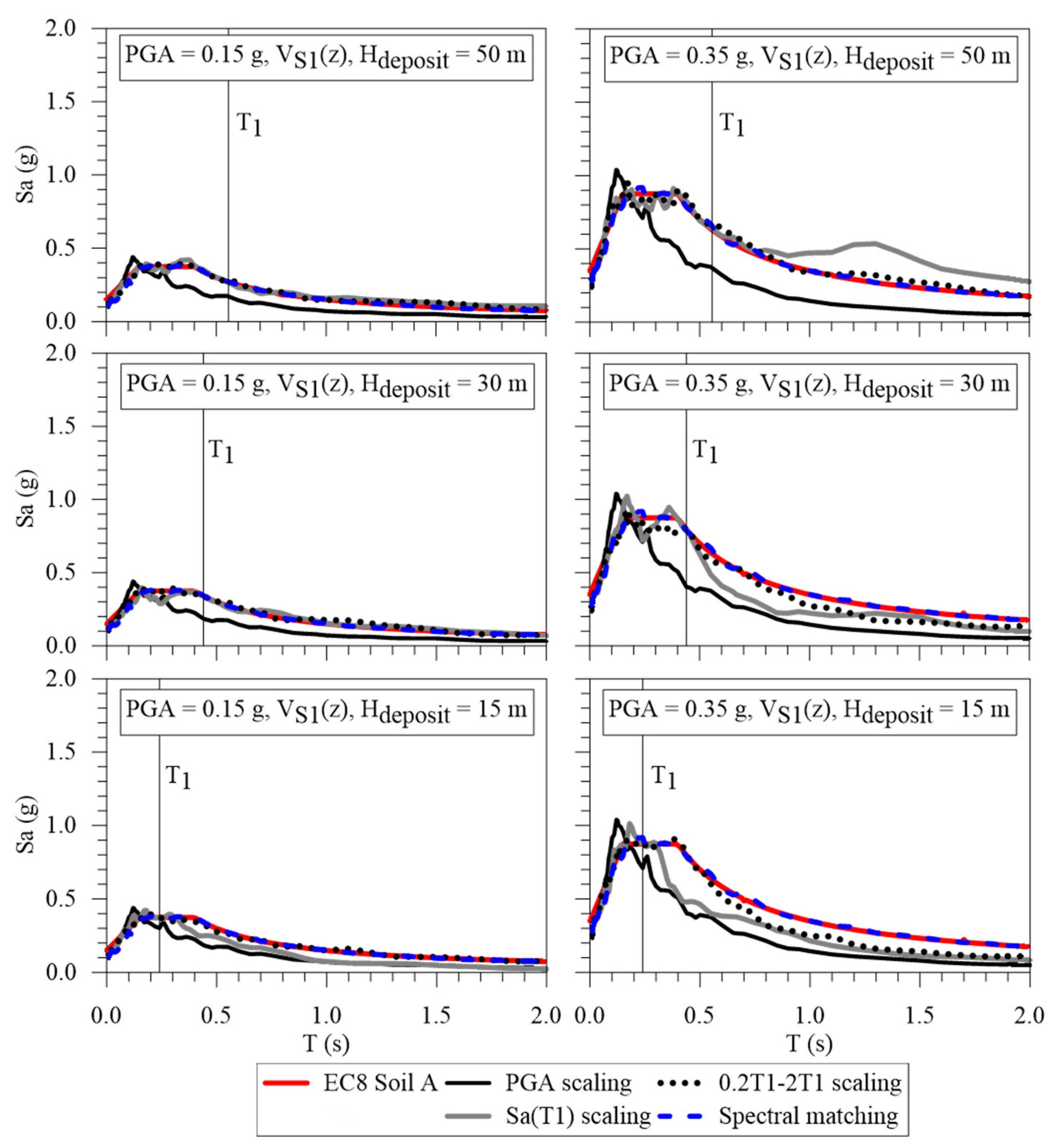
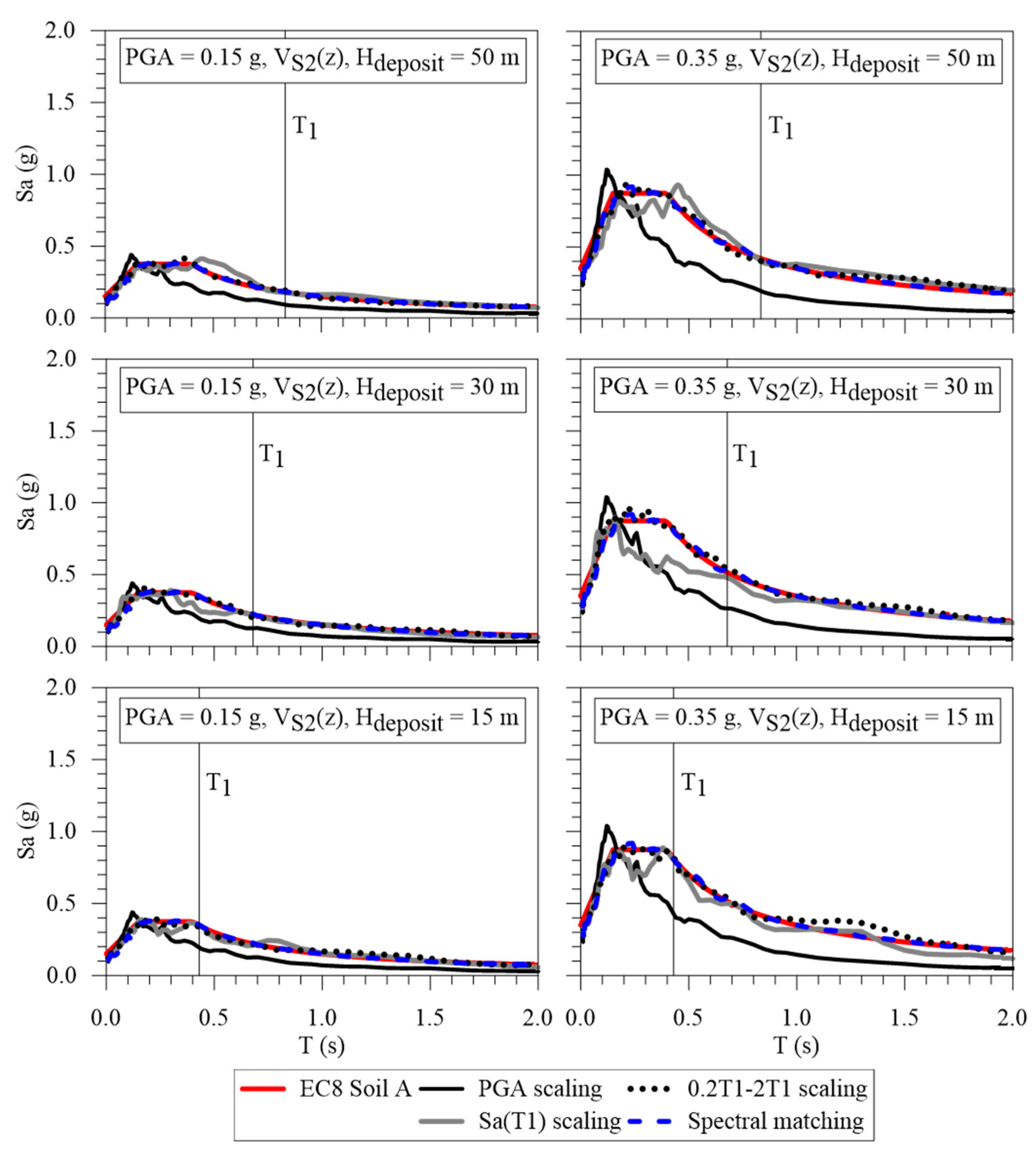
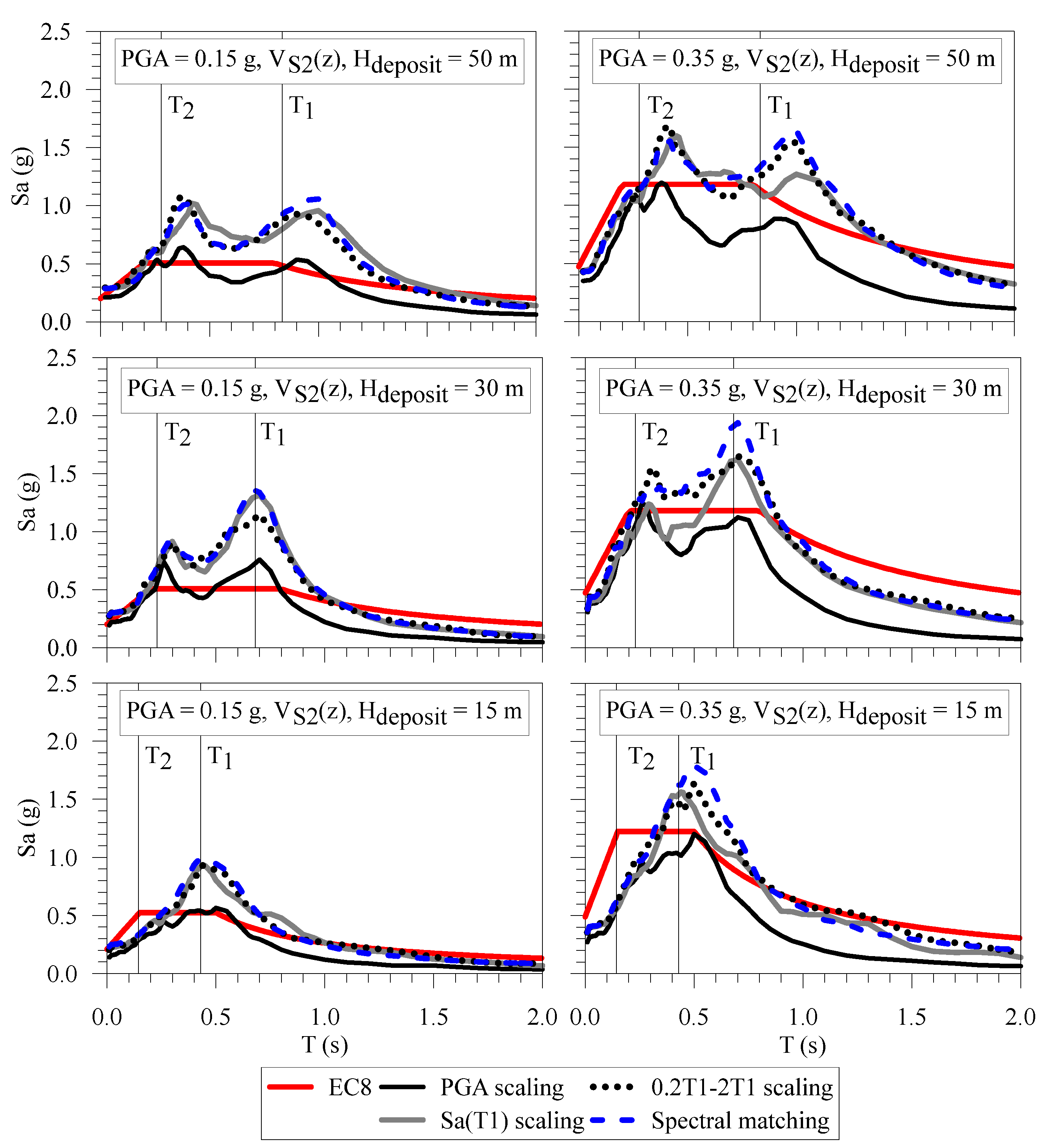
as Hdeposit increases, the number of vibration modes increases, as expected. In fact, the response spectra show only one peak close to T1 for Hdeposit = 15 m. On the other hand, two peaks in the response spectra can be identified when Hdeposit is equal to 50 m and 30 m;
-
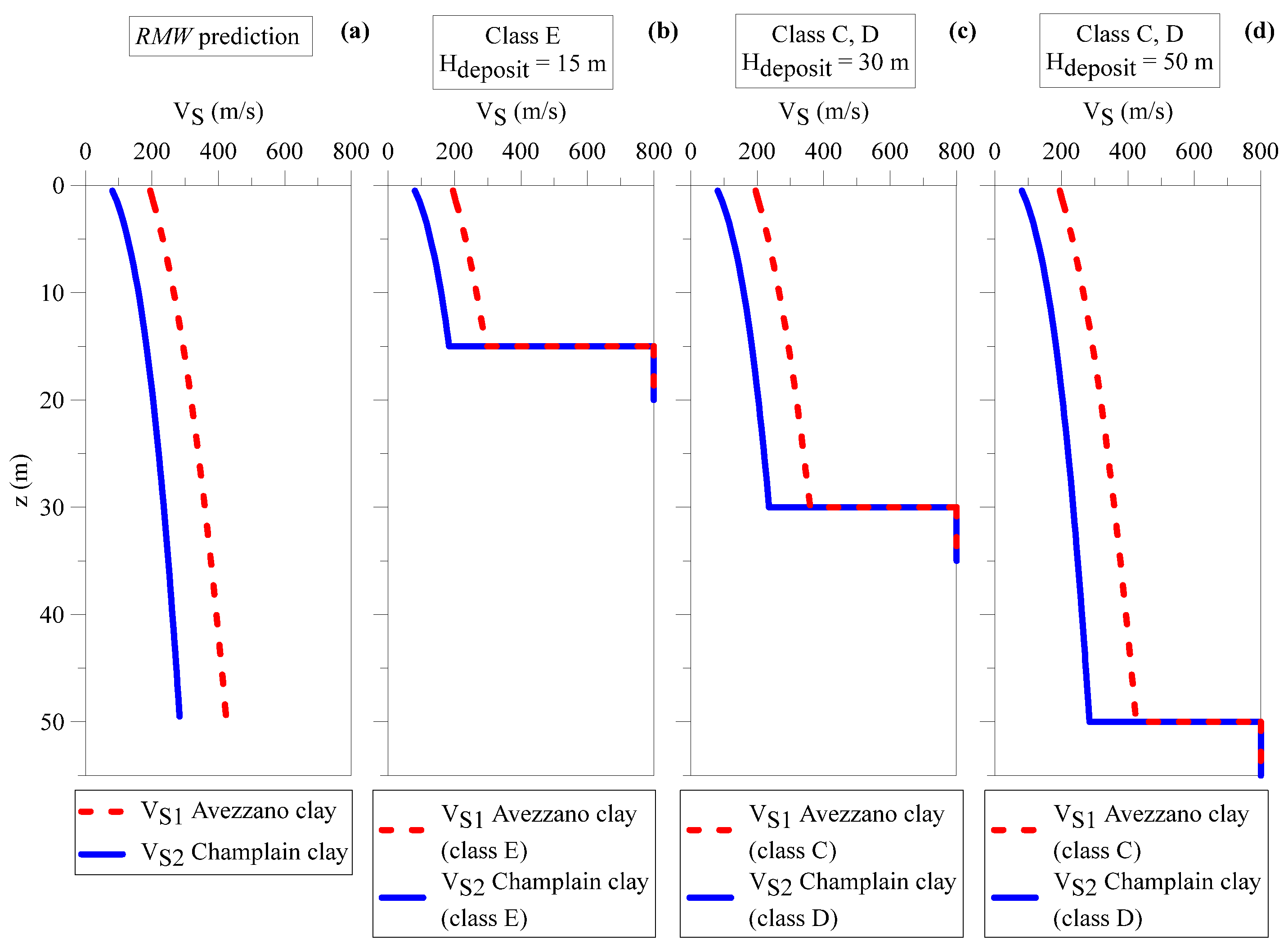
the first (T1) and second (T2) natural periods of vibration (i.e., the periods corresponding to the ground surface response spectra peaks) are higher when the column is deeper, as more nonlinear effects causing the elongation of the periods are expected to occur during the wave propagation process;
-
PGA scaling provides the lowest intensity ground surface response spectra, regardless of the assumed VS(z) profile, Hdeposit, and intensity level;
-
Sa(T1), 0.2T1-2T1, and full spectral matching supply similar ground surface response spectra, whatever VS(z) profile, Hdeposit, and PGA of the input motion are adopted;
-
the EC8 response spectra overestimate the LSSR results for T << T2 and T >> T1, while underestimation of the spectral accelerations is observed at the natural periods of vibration. Nevertheless, the EC8 design spectrum becomes a better proxy of the predicted surface response spectra in the case of earthquake events with higher intensity. This is also suggested by Rey et al. [62] and Pitilakis et al. [24], even though the values of PGA (i.e., Sa(T) at 0 s) are always overestimated by EC8.
Figure 5. Mean response spectra of the ground surface motions obtained by means of LSSR analyses considering the VS1(z) profile, 4 different selection strategies, and PGA equal to 0.15 g and 0.35 g. The EC8 response spectra going from the first to the bottom line refer to ground type C, C, and E, respectively.
Geosciences 13 00017 g005
Figure 6. Mean response spectra of the ground surface motions obtained by means of LSSR analyses considering the VS2(z) profile, 4 different selection strategies, and PGA equal to 0.15 g and 0.35 g. The EC8 response spectra going from the first to the bottom line refer to ground type D, D, and E, respectively.
Geosciences 13 00017 g006
Figure 7 and Figure 8 show the mean AFs for the Avezzano and Champlain clays deposits, respectively. The AFs, including the EC8 values, are calculated as:
AF Ta Tb = Ta Tb Sa o dT Ta Tb Sa i dT ,
where Sa is the pseudo-acceleration of the response spectra, and subscripts o and i refer to ground surface and input motion, respectively. Ta and Tb are the integration limits. Three period intervals are considered: 0.1–0.5 s, 0.4–0.8 s, and 0.7–1.1 s, which are commonly adopted in the Italian standards for seismic microzonation [63,64]. General comments for the studied cases are:
-
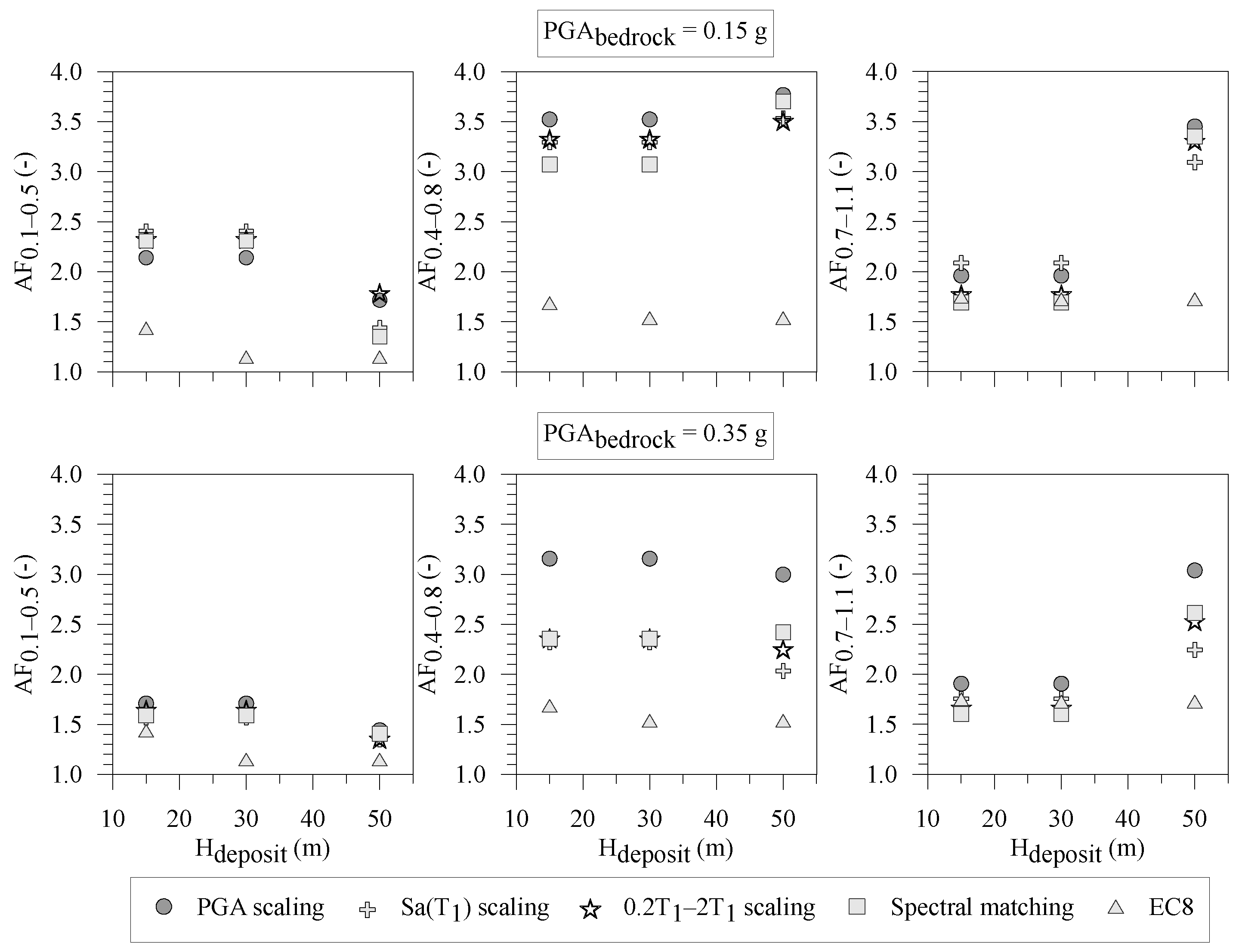
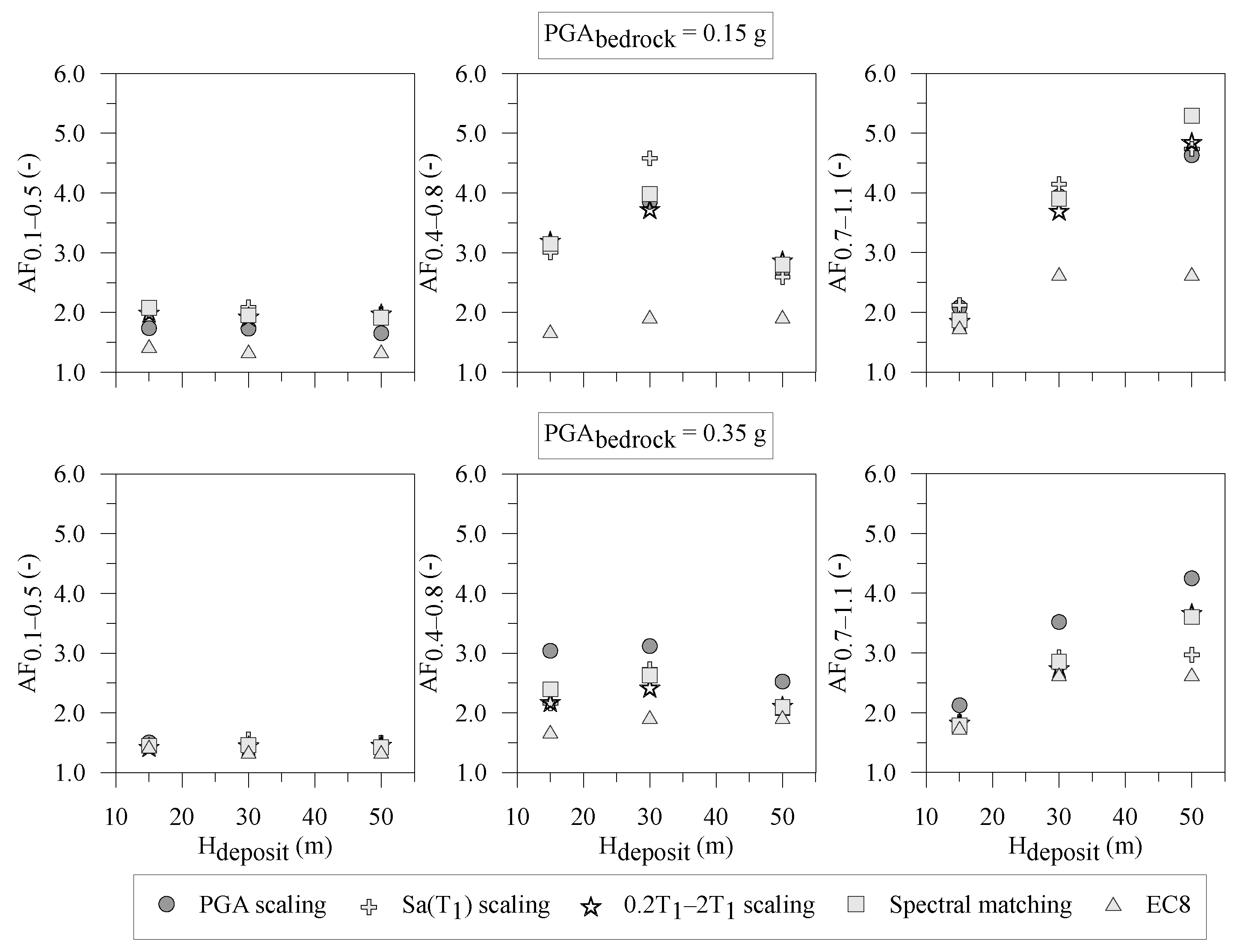
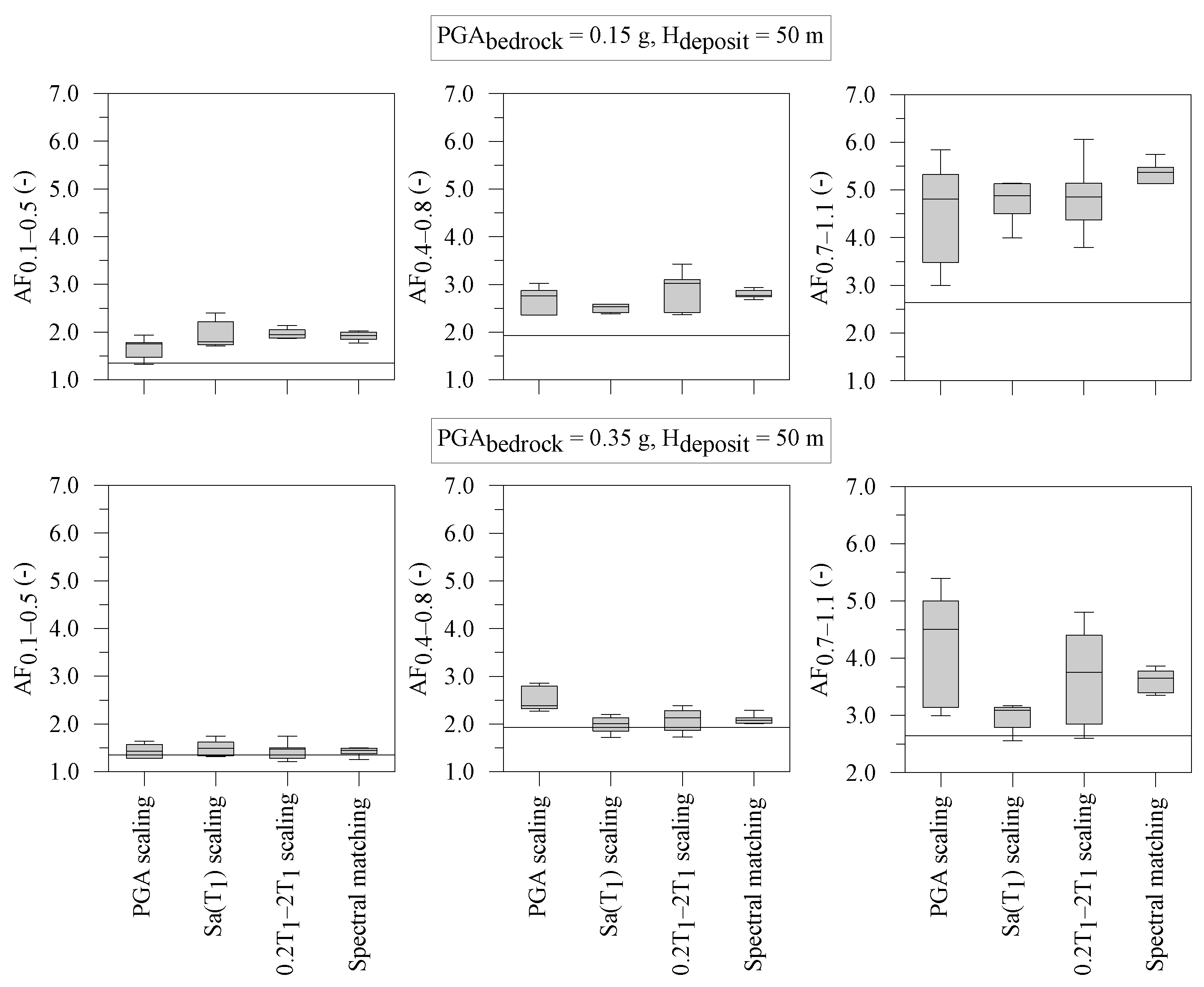
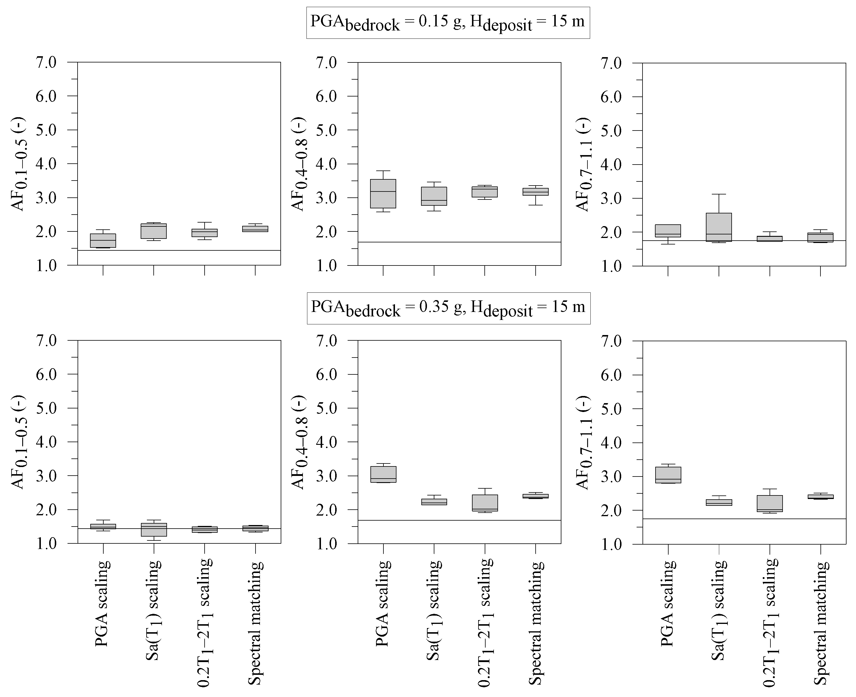
the mean values of the AFs obtained for the 0.15 g intensity level are larger than the corresponding ones obtained for the 0.35 g intensity level in all cases;
-
as Hdeposit increases, the AF0.1–0.5 values decrease. In contrast, as Hdeposit increases, the AF values for AF0.7–1.1 also increase, as already shown by Falcone and co-workers [27]. The trend of AF0.4–0.8 shows an intermediate behaviour: it is constant with respect to Hdeposit except in the cases where the PGA is equal to 0.15 g and VS2(z), where the highest values are gained for Hdeposit = 30 m (see Figure 8);
-
the EC8 AF trend with Hdeposit reproduces the behaviour discussed above. In fact, EC8 only distinguishes between Hdeposit lower than 30 m (i.e., class E deposits) and higher than 30 m (i.e., class C or D deposit);
-
within the 336 simulations, PGA scaling generally provides the highest AFs, while the EC8 values are usually the lowest.
Figure 7. Mean values of AFs for a deposit thickness equal to 15, 30, and 50 m, and VS1(z), considering 4 input motions selection strategies. EC8 values for 15, 30, and 50 m refer to ground types E, C, and C, respectively.
Geosciences 13 00017 g007
Figure 8. Mean values of AFs for a deposit thickness equal to 15, 30, and 50 m, and VS2(z), considering 4 input motions selection strategies. EC8 values for 15, 30, and 50 m refer to ground types E, D, and D, respectively.
Geosciences 13 00017 g008
Figure 9, Figure 10 and Figure 11 show the AFs box plots for the Avezzano clay deposits (i.e., VS1(z)) for each selection strategies, specifically the two PGA values of the input motion and the three selected Hdeposit (i.e., 15 m, 30 m, and 50 m). Figure 12, Figure 13 and Figure 14 show the AFs box plots for the Champlain clay deposits (i.e., VS2(z)). It should be noted that the upper and lower boundaries of the grey area (i.e., the box) are referred to as the 75th and 25th percentiles, respectively, while the whiskers (i.e., the lines outside the box) are obtained by multiplying the interquartile range (i.e., the distance between the upper and lower percentiles) by 1.5. Generally, it can be observed that:
-
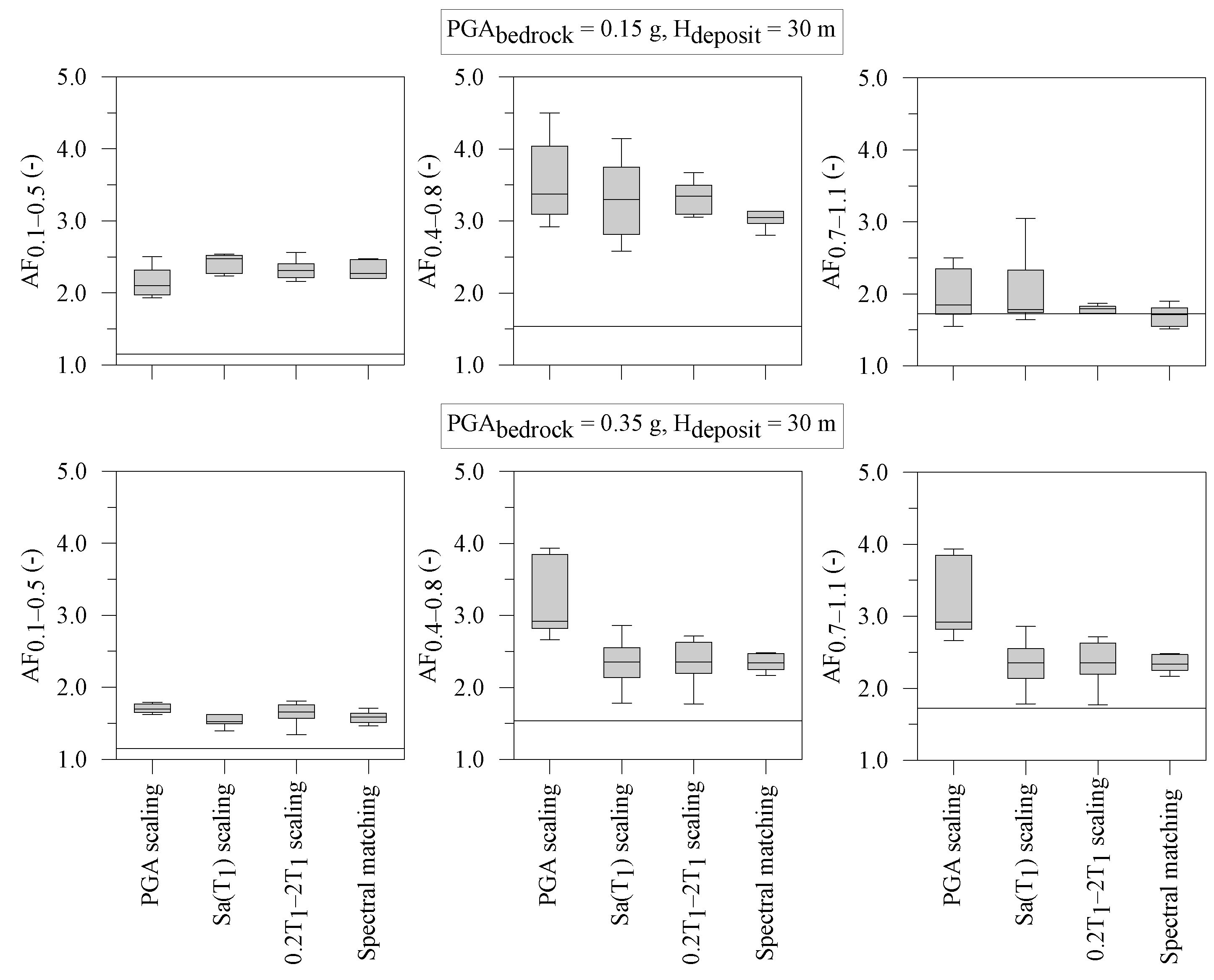
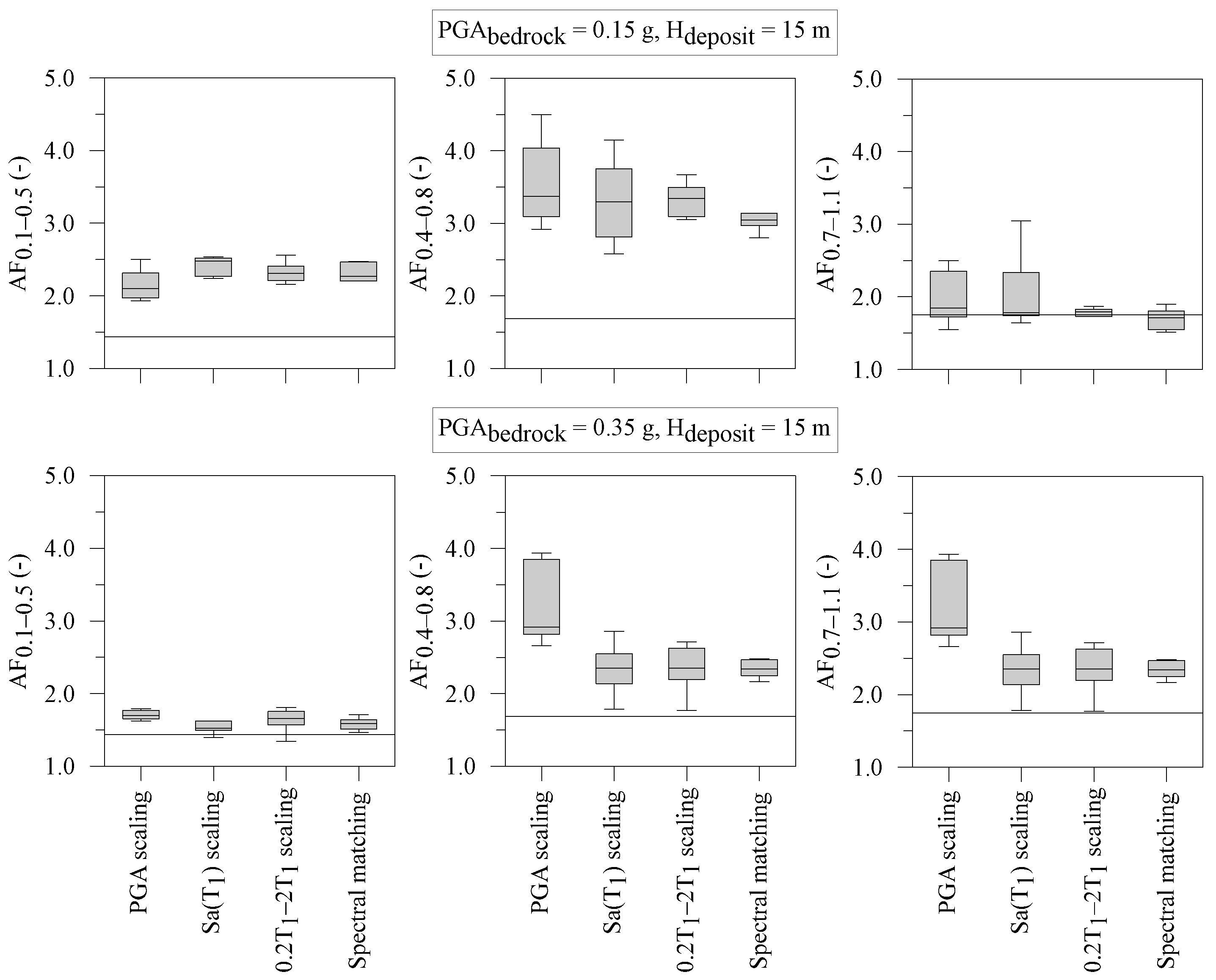
the EC8 AFs are the lowest, except for the cases of VS2(z), Hdeposit = 30 m, and PGA of the input motion equal to 0.35 g (Figure 13), for which the EC8 estimation is equal to about the mean value of the AF distribution provided by the LSSR analyses based on other selection strategies;
-
the AF0.1–0.5 distribution is characterised by the lowest variability;
-
within the 0.4–0.8 s and 0.7–1.1 s period ranges, the highest variability is observed when the PGA scaling strategy is used;
-
full spectral matching provides the lowest AF variability for all the examined case studies and selected period intervals.
Figure 9. Box plots of AFs for a deposit thickness equal to 50 m and VS1(z), considering 4 selection strategies for the input motions. The constant value retrieved from EC8 (thin black line) refers to ground type C.
Geosciences 13 00017 g009
Figure 10. Box plots of AFs for a deposit thickness equal to 30 m and VS1(z), considering 4 selection strategies for the input motions. The constant value retrieved from EC8 (thin black line) refers to ground type C.
Geosciences 13 00017 g010
Figure 11. Box plots of AFs for a deposit thickness equal to 15 m and VS1(z), considering 4 selection strategies for the input motions. The constant value retrieved from EC8 (thin black line) refers to ground type E.
Geosciences 13 00017 g011
Figure 12. Box plots of AFs for a deposit thickness equal to 50 m and VS2(z), considering 4 selection strategies for the input motions. The constant value retrieved from EC8 (thin black line) refers to ground type D.
Geosciences 13 00017 g012
Figure 13. Box plots of AFs for a deposit thickness equal to 30 m and VS2(z), considering 4 selection strategies for the input motions. The constant value retrieved from EC8 (thin black line) refers to ground type D.
Geosciences 13 00017 g013
Figure 14. Box plots of AFs for a deposit thickness equal to 15 m and VS2(z), considering 4 selection strategies for the input motions. The constant value retrieved from EC8 (thin black line) refers to ground type E.
Geosciences 13 00017 g014

5. Conclusions

Four different earthquake scaling strategies are chosen in this study to investigate the effect of the input motion characteristics on the results of free-field ground response analyses of ideal soft clay deposits with different thicknesses. For each scaling strategy, sets of seven bedrock motions, representing two seismic intensity levels (i.e., 0.15 g and 0.35 g), are generated using freely available computer programs. To account for the influence of soil nonlinearity on the wave propagation process, dynamic simulations are performed with a fully coupled effective stress-based FE code implementing an advanced elasto-plastic soil constitutive model. The results of more than 300 LSSR simulations are presented in terms of spectral response at ground surface and amplification factors. They are also compared with the corresponding EC8 predictions for soil classes C, D, and E.
The use of an advanced elasto-plastic soil constitutive model allows nonlinear ground response effects to be accounted for, including higher site amplification in the mid-period range and deamplification of the peak ground accelerations, due to plasticity during strong seismic actions. It is shown how these effects cannot be accurately captured by the simplified design code prescriptions. In particular, the spectral shape proposed by EC8 for soft soils tends to underestimate the surface response in the range between the first and the second natural periods of the soil column for low seismic intensity levels. EC8 design spectrum for soil classes D and E becomes a better proxy at higher intensity levels, even if a significant overprediction of the PGA is observed. Although the scope of this research is not to recommend new soil factors or a new spectral shape for soft soil deposits, the work would be useful for future revisions of the design codes, aimed at properly incorporating nonlinear site effects and the influence of the seismic bedrock depth.
Simply scaling the ground motion records at the same PGA does produce AF results that are not statistically matched with those obtained with more advanced scaling strategies. Therefore, PGA scaling should be avoided in the analysis of nonlinear ground response [51,52]. Even though the full spectral matching strategy implies a fictitious modification of the frequency content of natural records, statistically robust and stable mean AF values can be estimated by using spectrally matched accelerograms [51,52].
Bearing in mind that the AFs represent a potential supporting tool for urban planning and emergency systems, their quantifications over large areas should start from the definition of the appropriate bedrock motions scaling strategy in the period range of a structure. Seismic site response analyses over large areas are a non-trivial task since large uncertainties are linked to the soil type, soil and structure mechanical properties, stratigraphical succession, and building type, etc. With the aim of ensuring that the amplification phenomena are well predicted, regardless of the most recurrent building type in the area (which may be not known), 0.2T1-2T1 and full spectral matching should be preferred since the ground surface response variability is proved to be the lowest with respect to other explored selection strategies. In addition, the following general recommendations on the prediction of local seismic site response over large areas can be drawn from this research:
-
If the aim is to predict ground surface response spectra, the Sa(T1), 0.2T1-2T1, and full spectral matching strategies give similar results whatever shear wave profile, depth to the seismic bedrock, and peak ground acceleration of the input motion. PGA scaling should be avoided since it provides the lowest intensity ground surface response spectra;
-
If the target of the analysis over large areas is the determination of the mean amplification factors, the highest variability is observed when the PGA scaling strategy is adopted, whereas full spectral matching provides the lowest variability. The EC8 prescriptions appear to be generally nonconservative in the prediction of the AFs.

Supplementary Materials

The following supporting information can be downloaded at: https://www.mdpi.com/article/10.3390/geosciences13010017/s1, Figure S1: Response spectra in terms of pseudo-acceleration referred to input motions selected according to 4 selection strategies for PGA = 0.15 g and Soil C (i.e., VS1(z) for Hdeposit equal to 50 m); Figure S2: Response spectra in terms of pseudo-acceleration referred to input motions selected according to 4 selection strategies for PGA = 0.35 g and Soil C (i.e., VS1(z) for Hdeposit equal to 50 m); Figure S3: Response spectra in terms of pseudo-acceleration referred to input motions selected according to 4 selection strategies for PGA = 0.15 g and Soil C (i.e., VS1(z) for Hdeposit equal to 30 m); Figure S4: Response spectra in terms of pseudo-acceleration referred to input motions selected according to 4 selection strategies for PGA = 0.35 g and Soil C (i.e., VS1(z) for Hdeposit equal to 30 m); Figure S5: Response spectra in terms of pseudo-acceleration referred to input motions selected according to 4 selection strategies for PGA = 0.15 g and Soil E (i.e., VS1(z) for Hdeposit equal to 15 m); Figure S6: Response spectra in terms of pseudo-acceleration referred to input motions selected according to 4 selection strategies for PGA = 0.35 g and Soil E (i.e., VS1(z) for Hdeposit equal to 15 m); Figure S7: Response spectra in terms of pseudo-acceleration referred to input motions selected according to 4 selection strategies for PGA = 0.15 g and Soil D (i.e., VS2(z) for Hdeposit equal to 50 m); Figure S8: Response spectra in terms of pseudo-acceleration referred to input motions selected according to 4 selection strategies for PGA = 0.35 g and Soil D (i.e., VS2(z) for Hdeposit equal to 50 m); Figure S9: Response spectra in terms of pseudo-acceleration referred to input motions selected according to 4 selection strategies for PGA = 0.15 g and Soil D (i.e., VS2(z) for Hdeposit equal to 30 m); Figure S10: Response spectra in terms of pseudo-acceleration referred to input motions selected according to 4 selection strategies for PGA = 0.35 g and Soil D (i.e., VS2(z) for Hdeposit equal to 30 m); Figure S11: Response spectra in terms of pseudo-acceleration referred to input motions selected according to 4 selection strategies for PGA = 0.15 g and Soil E (i.e., VS2(z) for Hdeposit equal to 15 m); Figure S12: Response spectra in terms of pseudo-acceleration referred to input motions selected according to 4 selection strategies for PGA = 0.35 g and Soil E (i.e., VS2(z) for Hdeposit equal to 15 m); Figure S13: Response spectra in terms of pseudo-acceleration referred to the ground surface motions obtained by means of the LSSR analysis considering the input motions from the 4 selection strategies for PGA = 0.15 g and Soil C (i.e., VS1(z) for Hdeposit equal to 50 m); Figure S14: Response spectra in terms of pseudo-acceleration referred to the ground surface motions obtained by means of the LSSR analysis considering the input motions from the 4 selection strategies for PGA = 0.35 g and Soil C (i.e., VS1(z) for Hdeposit equal to 50 m); Figure S15: Response spectra in terms of pseudo-acceleration referred to the ground surface motions obtained by means of the LSSR analysis considering the input motions from the 4 selection strategies for PGA = 0.15 g and Soil C (i.e., VS1(z) for Hdeposit equal to 30 m); Figure S16: Response spectra in terms of pseudo-acceleration referred to the ground surface motions obtained by means of the LSSR analysis considering the input motions from the 4 selection strategies for PGA = 0.35 g and Soil C (i.e., VS1(z) for Hdeposit equal to 30 m); Figure S17. Response spectra in terms of pseudo-acceleration referred to the ground surface motions obtained by means of the LSSR analysis considering the input motions from the 4 selection strategies for PGA = 0.15 g and Soil E (i.e., VS1(z) for Hdeposit equal to 15 m); Figure S18: Response spectra in terms of pseudo-acceleration referred to the ground surface motions obtained by means of the LSSR analysis considering the input motions from the 4 selection strategies for PGA = 0.35 g and Soil E (i.e., VS1(z) for Hdeposit equal to 15 m); Figure S19: Response spectra in terms of pseudo-acceleration referred to the ground surface motions obtained by means of the LSSR analysis considering the input motions from the 4 selection strategies for PGA = 0.15 g and Soil D (i.e., VS2(z) for Hdeposit equal to 50 m); Figure S20: Response spectra in terms of pseudo-acceleration referred to the ground surface motions obtained by means of the LSSR analysis considering the input motions from the 4 selection strategies for PGA = 0.35 g and Soil D (i.e., VS2(z) for Hdeposit equal to 50 m); Figure S21: Response spectra in terms of pseudo-acceleration referred to the ground surface motions obtained by means of the LSSR analysis considering the input motions from the 4 selection strategies for PGA = 0.15 g and Soil D (i.e., VS2(z) for Hdeposit equal to 30 m); Figure S22: Response spectra in terms of pseudo-acceleration referred to the ground surface motions obtained by means of the LSSR analysis considering the input motions from the 4 selection strategies for PGA = 0.35 g and Soil D (i.e., VS2(z) for Hdeposit equal to 30 m); Figure S23: Response spectra in terms of pseudo-acceleration referred to the ground surface motions obtained by means of the LSSR analysis considering the input motions from the 4 selection strategies for PGA = 0.15 g and Soil E (i.e., VS2(z) for Hdeposit equal to 15 m); Figure S24: Response spectra in terms of pseudo-acceleration referred to the ground surface motions obtained by means of the LSSR analysis considering the input motions from the 4 selection strategies for PGA = 0.35 g and Soil E (i.e., VS2(z) for Hdeposit equal to 15 m). Table S1: Main characteristics of the selected earthquake signals based on Sa(T1) scaling, 0.2T1-2T1 scaling, and full spectral matching for 0.15 g intensity level, VS1(z) and Hdeposit = 50 m; Table S2: Main characteristics of the selected earthquake signals based on Sa(T1) scaling, 0.2T1-2T1 scaling, and full spectral matching for 0.35 g intensity level, VS1(z) and Hdeposit = 50 m; Table S3: Main characteristics of the selected earthquake signals based on Sa(T1) scaling, 0.2T1-2T1 scaling, and full spectral matching for 0.15 g intensity level, VS1(z) and Hdeposit = 30 m; Table S4: Main characteristics of the selected earthquake signals based on Sa(T1) scaling, 0.2T1-2T1 scaling, and full spectral matching for 0.35 g intensity level, VS1(z) and Hdeposit = 30 m; Table S5: Main characteristics of the selected earthquake signals based on Sa(T1) scaling, 0.2T1-2T1 scaling, and full spectral matching for 0.15 g intensity level, VS1(z) and Hdeposit = 15 m; Table S6: Main characteristics of the selected earthquake signals based on Sa(T1) scaling, 0.2T1-2T1 scaling, and full spectral matching for 0.35 g intensity level, VS1(z) and Hdeposit = 15 m; Table S7: Main characteristics of the selected earthquake signals based on Sa(T1) scaling, 0.2T1-2T1 scaling, and full spectral matching for 0.15 g intensity level, VS2(z) and Hdeposit = 50 m; Table S8: Main characteristics of the selected earthquake signals based on Sa(T1) scaling, 0.2T1-2T1 scaling, and full spectral matching for 0.35 g intensity level, VS2(z) and Hdeposit = 50 m; Table S9: Main characteristics of the selected earthquake signals based on Sa(T1) scaling, 0.2T1-2T1 scaling, and full spectral matching for 0.15 g intensity level, VS2(z) and Hdeposit = 30 m; Table S10: Main characteristics of the selected earthquake signals based on Sa(T1) scaling, 0.2T1-2T1 scaling, and full spectral matching for 0.35 g intensity level, VS2(z) and Hdeposit = 30 m; Table S11: Main characteristics of the selected earthquake signals based on Sa(T1) scaling, 0.2T1-2T1 scaling, and full spectral matching for 0.15 g intensity level, VS2(z) and Hdeposit = 15 m; Table S12: Main characteristics of the selected earthquake signals based on Sa(T1) scaling, 0.2T1-2T1 scaling, and full spectral matching for 0.35 g intensity level, VS2(z) and Hdeposit = 15 m; Table S13: Main characteristics of the selected earthquake signals based on PGA scaling for 0.15 g intensity level, VS1(z) and Hdeposit = 15, 30, and 50 m; Table S14: Main characteristics of the selected earthquake signals based on PGA scaling for 0.35 g intensity level, VS2(z) and Hdeposit = 15, 30, and 50 m.

Author Contributions

Conceptualization, Y.G., G.E. and M.R.; methodology, Y.G., G.E. and M.R.; formal analysis, Y.G. and G.E.; data curation, Y.G. and G.F.; writing—original draft preparation, Y.G., G.E., M.R. and G.F.; writing—review and editing, Y.G., G.E., M.R. and G.F.; visualization, Y.G. and G.F.; supervision, G.E. and M.R.; project administration, G.E. and M.R. All authors have read and agreed to the published version of the manuscript.

Funding

This research received no external funding.

Data Availability Statement

The data presented in this study are available in Supplementary Material.

Acknowledgments

The first author would like to acknowledge the support received from the Ministry of National Education—Republic of Turkey for his Ph.D. studies at Newcastle University. The support received by the last author from the PON—MITIGO project is also acknowledged. The authors would like to thank the editor and the two anonymous reviewers for their helpful comments and suggestion which have improved the final paper.

Conflicts of Interest

The authors declare no conflict of interest.

References

  1. Fayjaloun, R.; Negulescu, C.; Roullé, A.; Auclair, S.; Gehl, P.; Faravelli, M.; Abrahamczyk, L.; Petrovčič, S.; Martinez-Frias, J. Sensitivity of Earthquake Damage Estimation to the Input Data (Soil Characterization Maps and Building Exposure): Case Study in the Luchon Valley, France. Geosciences 2021, 11, 249. [Google Scholar] [CrossRef]
  2. Kwok, A.O.L.; Stewart, J.P.; Hashash, Y.M.A.; Matasovic, N.; Pyke, R.; Wang, Z.; Yang, Z. Use of Exact Solutions of Wave Propagation Problems to Guide Implementation of Nonlinear Seismic Ground Response Analysis Procedures. J. Geotech. Geoenvironmental Eng. 2007, 133, 1385–1398. [Google Scholar] [CrossRef] [Green Version]
  3. Amorosi, A.; Boldini, D.; Elia, G. Parametric Study on Seismic Ground Response by Finite Element Modelling. Comput. Geotech. 2010, 37, 515–528. [Google Scholar] [CrossRef]
  4. Nikolopoulos, D.; Mascandola, C.; Lanzano, G.; Pacor, F. Consistency Check of ITACAext, the Flatfile of the Italian Accelerometric Archive. Geosciences 2022, 12, 334. [Google Scholar] [CrossRef]
  5. Falcone, G.; Romagnoli, G.; Naso, G.; Mori, F.; Peronace, E.; Moscatelli, M. Effect of Bedrock Stiffness and Thickness on Numerical Simulation of Seismic Site Response. Italian Case Studies. Soil Dyn. Earthq. Eng. 2020, 139, 106361. [Google Scholar] [CrossRef]
  6. Kokusho, T.; Ishizawa, T.; Martinez-Frias, J.; Nappi, R. Site Amplification during Strong Earthquakes Investigated by Vertical Array Records. Geosciences 2021, 11, 510. [Google Scholar] [CrossRef]
  7. Griffiths, S.C.; Cox, B.R.; Rathje, E.M.; Teague, D.P. Mapping Dispersion Misfit and Uncertainty in Vs Profiles to Variability in Site Response Estimates. J. Geotech. Geoenvironmental Eng. 2016, 142. [Google Scholar] [CrossRef]
  8. Phoon, K.K.; Kulhawy, F.H. Characterization of Geotechnical Variability. Can. Geotech. J. 2011, 36, 612–624. [Google Scholar] [CrossRef]
  9. Romagnoli, G.; Tarquini, E.; Porchia, A.; Catalano, S.; Albarello, D.; Moscatelli, M. Constraints for the Vs Profiles from Engineering-Geological Qualitative Characterization of Shallow Subsoil in Seismic Microzonation Studies. Soil Dyn. Earthq. Eng. 2022, 161, 107347. [Google Scholar] [CrossRef]
  10. Rathje, E.M.; Kottke, A.R.; Trent, W.L. Influence of Input Motion and Site Property Variabilities on Seismic Site Response Analysis. J. Geotech. Geoenvironmental Eng. 2010, 136, 607–619. [Google Scholar] [CrossRef]
  11. Bazzurro, P.; Cornell, C.A. Ground-Motion Amplification in Nonlinear Soil Sites with Uncertain Properties. Bull. Seismol. Soc. Am. 2004, 94, 2090–2109. [Google Scholar] [CrossRef]
  12. Stewart, J.P.; Kwok, A.O.L. Nonlinear Seismic Ground Response Analysis: Code Usage Protocols and Verification against Vertical Array Data. Am. Soc. Civ. Eng. 2008, 1–24. [Google Scholar] [CrossRef] [Green Version]
  13. Guzel, Y.; Rouainia, M.; Elia, G. Effect of Soil Variability on Nonlinear Site Response Predictions: Application to the Lotung Site. Comput. Geotech 2020, 121, 103444. [Google Scholar] [CrossRef]
  14. Shome, N.; Cornell, C.A.; Bazzurro, P.; Carballo, J.E. Earthquakes, Records, and Nonlinear Responses. Earthq. Spectra 1998, 14, 469–500. [Google Scholar] [CrossRef]
  15. Eurocode 8: Design of Structures for Earthquake Resistance|Eurocodes: Building the Future. Available online: https://eurocodes.jrc.ec.europa.eu/EN-Eurocodes/eurocode-8-design-structures-earthquake-resistance (accessed on 14 September 2022).
  16. Hancock, J.; Watson-Lamprey, J.; Abrahamson, N.A.; Bommer, J.J.; Markatis, A.; McCoy, E.M.M.A.; Mendis, R. An Improved Method of Matching Response Spectra of Recorded Earthquake Ground Motion Using Wavelets. J. Earthq. Eng. 2006, 10, 67–89. [Google Scholar] [CrossRef]
  17. Haselton, C.B. Evaluation of Ground Motion Selection and Modification Methods: Predicting Median Interstory Drift Response of Buildings; Pacific Earthquake Engineering Research Center, University of California: Berkeley, CA, USA, 2009. [Google Scholar]
  18. Galasso, C. Consolidating Record Selection for Earthquake Resistant Structural Design. Ph.D. Thesis, Università degli Studi di Napoli Federico II, Napoli, Italy, 2010. [Google Scholar]
  19. Kottke, A.; Rathje, E.M. A Semi-Automated Procedure for Selecting and Scaling Recorded Earthquake Motions for Dynamic Analysis. Earthq. Spectra 2008, 24, 911–932. [Google Scholar] [CrossRef]
  20. Tönük, G.; Ansal, A.; Kurtuluş, A.; Çetiner, B. Site Specific Response Analysis for Performance Based Design Earthquake Characteristics. Bull. Earthq. Eng. 2014, 12, 1091–1105. [Google Scholar] [CrossRef]
  21. Amirzehni, E.; Taiebat, M.; Finn, W.D.L.; DeVall, R.H. Ground Motion Scaling/Matching for Nonlinear Dynamic Analysis of Basement Walls. In Proceedings of the 11th Canadian Conference on Earthquake Engineering, Victoria, BC, USA, 21–24 July 2015. [Google Scholar]
  22. Elia, G.; di Lernia, A.; Rouainia, M. Ground Motion Scaling for the Assessment of the Seismic Response of a Diaphragm Wall. In Earthquake Geotechnical Engineering for Protection and Development of Environment and Constructions, Proceedings of the 7th International Conference on Earthquake Geotechnical Engineering, Rome, Italy, 17–20 June, 2019; CRC Press: Boca Raton, FL, USA, 2019; pp. 2249–2257. [Google Scholar]
  23. Mazzoni, S.; Hachem, M.; Sinclair, M. An Improved Approach for Ground Motion Suite Selection and Modification for Use in Response History Analysis. In Proceedings of the 15th World Conference on Earthquake Engineering, Lisbon, Portugal, 24–28 September 2012. [Google Scholar]
  24. Pitilakis, K.; Riga, E.; Anastasiadis, A. Design Spectra and Amplification Factors for Eurocode 8. Bull. Earthq. Eng. 2012, 10, 1377–1400. [Google Scholar] [CrossRef]
  25. Guzel, Y. Influence of Input Motion Selection and Soil Variability on Nonlinear Ground Response Analyses. Ph.D. Thesis, Newcastle University, Newcastle, UK, 2018. [Google Scholar]
  26. Moscatelli, M.; Albarello, D.; Mugnozza, G.S.; Dolce, M. The Italian Approach to Seismic Microzonation. Bull. Earthq. Eng. 2020, 18, 5425–5440. [Google Scholar] [CrossRef]
  27. Falcone, G.; Acunzo, G.; Mendicelli, A.; Mori, F.; Naso, G.; Peronace, E.; Porchia, A.; Romagnoli, G.; Tarquini, E.; Moscatelli, M. Seismic Amplification Maps of Italy Based on Site-Specific Microzonation Dataset and One-Dimensional Numerical Approach. Eng. Geol. 2021, 289, 106170. [Google Scholar] [CrossRef]
  28. Mendicelli, A.; Falcone, G.; Acunzo, G.; Mori, F.; Naso, G.; Peronace, E.; Porchia, A.; Romagnoli, G.; Moscatelli, M. Italian Seismic Amplification Factors for Peak Ground Acceleration and Peak Ground Velocity. J. Maps 2022, 18, 497–507. [Google Scholar] [CrossRef]
  29. Chan, A.H.C. User Manual for DIANA-SWANDYNE II; School of Engineering, Univ. of Birmingham: Birmingham, UK, 1995. [Google Scholar]
  30. Biot, M.A. General Theory of Three-Dimensional Consolidation. J. Appl. Phys. 1941, 12, 155–164. [Google Scholar] [CrossRef]
  31. Zienkiewicz, O.C.; Chan, A.H.C.; Pastor, M.; Schrefler, B.A.; Shiomi, T. Computational Geomechanics with Special Reference to Earthquake Engineering; John Wiley & Sons: Chichester, UK, 1999; ISBN 978-0-471-98285-2. [Google Scholar]
  32. Rouainia, M.; Wood, D.M. A Kinematic Hardening Constitutive Model for Natural Clays with Loss of Structure. Géotechnique 2000, 50, 153–164. [Google Scholar] [CrossRef]
  33. Elia, G.; Rouainia, M. Seismic Performance of Earth Embankment Using Simple and Advanced Numerical Approaches. J. Geotech. Geoenvironmental Eng. 2013, 139, 1115–1129. [Google Scholar] [CrossRef]
  34. Elia, G.; Rouainia, M. Performance Evaluation of a Shallow Foundation Built on Structured Clays under Seismic Loading. Bull. Earthq. Eng. 2014, 12, 1537–1561. [Google Scholar] [CrossRef] [Green Version]
  35. Elia, G.; Rouainia, M.; Karofyllakis, D.; Guzel, Y. Modelling the Non-Linear Site Response at the LSST down-Hole Accelerometer Array in Lotung. Soil Dyn. Earthq. Eng. 2017, 102, 1–14. [Google Scholar] [CrossRef] [Green Version]
  36. Elia, G.; Rouainia, M. Investigating the Cyclic Behaviour of Clays Using a Kinematic Hardening Soil Model. Soil Dyn. Earthq. Eng. 2016, 88, 399–411. [Google Scholar] [CrossRef]
  37. D’Elia, M. Comportamento Meccanico in Condizioni Cicliche e Dinamiche Di Un’argilla Naturale Cementata. Ph.D. Thesis, University of Rome ‘“La Sapienza”, Roma, Italy, 2001. [Google Scholar]
  38. Chehat, A.; Hussien, M.N.; Abdellaziz, M.; Chekired, M.; Harichane, Z.; Karray, M. Stiffness– and Damping–Strain Curves of Sensitive Champlain Clays through Experimental and Analytical Approaches. Can. Geotech. J. 2019, 56, 364–377. [Google Scholar] [CrossRef] [Green Version]
  39. Panayides, S.; Rouainia, M.; Wood, D.M. Influence of Degradation of Structure on the Behaviour of a Full-Scale Embankment. Can. Geotech. J. 2012, 49, 344–356. [Google Scholar] [CrossRef]
  40. Leroueil, S.; Vaughan, P.R. The General and Congruent Effects of Structure in Natural Soils and Weak Rocks. Geotechnique 1990, 40, 467–488. [Google Scholar] [CrossRef]
  41. Tavenas, F.A.; Chapeau, C.; la Rochelle, P.; Roy, M. Immediate settlements of three test embankments on Champlain clay. Can. Geotech. J. 1974, 11, 109–141. [Google Scholar] [CrossRef]
  42. Cabangon, L.T.; Elia, G.; Rouainia, M. Modelling the Transverse Behaviour of Circular Tunnels in Structured Clayey Soils during Earthquakes. Acta Geotech. 2022, 14, 163–178. [Google Scholar] [CrossRef] [Green Version]
  43. Falcone, G.; Boldini, D.; Amorosi, A. Site Response Analysis of an Urban Area: A Multi-Dimensional and Non-Linear Approach. Soil Dyn. Earthq. Eng. 2018, 109, 33–45. [Google Scholar] [CrossRef]
  44. Régnier, J.; Bonilla, L.; Bard, P.; Bertrand, E.; Hollender, F.; Kawase, H.; Sicilia, D.; Arduino, P.; Amorosi, A.; Asimaki, D.; et al. International Benchmark on Numerical Simulations for 1D, Nonlinear Site Response (PRENOLIN): Verification Phase Based on Canonical Cases. Bull. Seismol. Soc. Am. 2016, 106, 2112–2135. [Google Scholar] [CrossRef]
  45. Clough, R.W.; Penzien, J. Dynamics of Structures; Computers & Structures, Inc.: Berkley, CA, USA, 1995. [Google Scholar]
  46. Vucetic, M.; Dobry, R. Effect of Soil Plasticity on Cyclic Response. J. Geotech. Eng. 1991, 117, 89–107. [Google Scholar] [CrossRef]
  47. Viggiani, G.; Atkinson, J.H. Stiffness of Fine-Grained Soil at Very Small Strains. Géotechnique 1995, 45, 249–265. [Google Scholar] [CrossRef]
  48. Darendeli, M.B. Development of a New Family of Normalized Modulus Reduction and Material Damping Curves. Ph.D. Thesis, The University of Texas at Austin, Austin, TX, USA, 2001. [Google Scholar]
  49. Régnier, J.; Bonilla, L.; Bard, P.; Bertrand, E.; Hollender, F.; Kawase, H.; Sicilia, D.; Arduino, P.; Amorosi, A.; Asimaki, D.; et al. PRENOLIN: International Benchmark on 1D Nonlinear Site-Response Analysis—Validation Phase Exercise. Bull. Seismol. Soc. Am. 2018, 108, 876–900. [Google Scholar] [CrossRef] [Green Version]
  50. Di Lernia, A.; Amorosi, A.; Boldini, D. A Multi-Directional Numerical Approach for the Seismic Ground Response and Dynamic Soil-Structure Interaction Analyses. In Earthquake Geotechnical Engineering for Protection and Development of Environment and Constructions, Proceedings of the 7th International Conference on Earthquake Geotechnical Engineering, Rome, Italy, 17–20 June 2019; CRC Press: Boca Raton, FL, USA, 2019; pp. 2145–2152. [Google Scholar]
  51. Callisto, L.; Rampello, S.; Viggiani, G.M.B. Soil–Structure Interaction for the Seismic Design of the Messina Strait Bridge. Soil Dyn. Earthq. Eng. 2013, 52, 103–115. [Google Scholar] [CrossRef] [Green Version]
  52. Mejia, L.H.; Dawson, E.M. Earthquake Deconvolution for FLAC. In Proceedings of the 4th International FLAC Symposium on Numerical Modeling in Geomechanics, Madrid, Spain, 29–31 May 2006; Itasca Consulting Group: Minneapolis, MN, USA, 2006. [Google Scholar]
  53. Falcone, G.; Naso, G.; Mori, F.; Mendicelli, A.; Acunzo, G.; Peronace, E.; Moscatelli, M. Effect of Base Conditions in One-Dimensional Numerical Simulation of Seismic Site Response: A Technical Note for Best Practice. GeoHazards 2021, 2, 430–441. [Google Scholar] [CrossRef]
  54. Kumar, N.; Narayan, J.P. Quantification of Site-City Interaction Effects on the Response of Structure under Double Resonance Condition. Geophys. J. Int. 2018, 212, 422–441. [Google Scholar] [CrossRef]
  55. Kham, M.; Semblat, J.F.; Bard, P.Y.; Dangla, P. Seismic Site–City Interaction: Main Governing Phenomena through Simplified Numerical Models. Bull. Seismol. Soc. Am. 2006, 96, 1934–1951. [Google Scholar] [CrossRef]
  56. Kramer, S. Geotechnical Earthquake Engineering; Prentice Hall: Upper Saddle River, NJ, USA, 1996; ISBN 9780133749434. [Google Scholar]
  57. Abrahamson, N.A. Non-Stationary Spectral Matching. Seismol. Res. Lett. 1992, 63, 30. [Google Scholar]
  58. Ambraseys, N.; Smit, P.; Sigbjornsson, R.; Suhadolc, P.; Margaris, B. Internet-Site for European Strong-Motion Data. Boll. Di Geofis. Teor. Ed Appl. 2004, 45, 113–129. [Google Scholar]
  59. Iervolino, I.; Galasso, C.; Cosenza, E. REXEL: Computer Aided Record Selection for Code-Based Seismic Structural Analysis. Bull. Earthq. Eng. 2009, 8, 339–362. [Google Scholar] [CrossRef]
  60. Bommer, J.J.; Acevedo, A.B. The Use of Real Earthquake Accelerograms as Input to Dynamic Analysis. J. Earthq. Eng. 2004, 8, 43. [Google Scholar] [CrossRef]
  61. SeismoMatch a Computer Program for Spectrum Matching of Earthquake Records. 2016. Available online: http://www.seismosoft.com (accessed on 25 April 2018).
  62. Rey, J.; Faccioli, E.; Bommer, J.J. Derivation of Design Soil Coefficients (S) and Response Spectral Shapes for Eurocode 8 Using the European Strong-Motion Database. J Seism. 2002, 6, 547–555. [Google Scholar] [CrossRef]
  63. Falcone, G.; Boldini, D.; Martelli, L.; Amorosi, A. Quantifying Local Seismic Amplification from Regional Charts and Site Specific Numerical Analyses: A Case Study. Bull. Earthq. Eng. 2020, 18, 77–107. [Google Scholar] [CrossRef]
  64. Falcone, G.; Mendicelli, A.; Mori, F.; Fabozzi, S.; Moscatelli, M.; Occhipinti, G.; Peronace, E. A Simplified Analysis of the Total Seismic Hazard in Italy. Eng. Geol. 2020, 267, 105511. [Google Scholar] [CrossRef]
Figure 2. Shear wave velocity profiles adopted in the FE simulations: (a) RMW predictions based on the Viggiani and Atkinson formula (i.e., Equation (1)), (b) class E thin deposits (VS30 < 360 m/s, Hdeposit = 15 m), (c) classes C and D shallow deposits (VS30 < 360 m/s, Hdeposit = 30 m), and (d) class C and D deep deposits (VS30 < 360 m/s, Hdeposit = 50 m). In the figure, the EC8 soil class is also included for each considered deposit. Hdeposit stands for the depth of the seismic bedrock.
Geosciences 13 00017 g002
Figure 3. Mean response spectra of the input motions selected, according to 4 different selection strategies for PGA equal to 0.15 g and 0.35 g, and VS1(z) profile. The response spectra going from the first line to the bottom one refers to a Hdeposit equal to 50, 30, and 15 m, respectively.
Geosciences 13 00017 g003
Figure 4. Mean response spectra of the input motions selected according to 4 different selection strategies for PGA equal to 0.15 g and 0.35 g, and VS2(z) profile. The response spectra going from the first line to the bottom one refers to a Hdeposit equal to 50, 30, and 15 m, respectively.
Geosciences 13 00017 g004
Table 1. RMW parameters for Avezzano and Champlain clays.
Parameter/SymbolPhysical Contribution/MeaningAvezzanoChamplain
MCritical state stress ratio for triaxial compression1.421.07
λ *Slope of normal compression line in ln(v)-ln(p) compression plane0.110.215
κ *Slope of swelling line in ln(v)-ln(p) compression plane0.0160.005
RRatio of size of bubble and reference surface0.40.11
BStiffness interpolation parameter15.01.0
ψStiffness interpolation exponent1.451.6
η0Anisotropy of initial structure00.3
r0Initial degree of structure5.22.1
A*Parameter controlling relative proportion of distorsional and volumetric destructuration0.20.75
kParameter controlling rate of destructuration with damage strain1.55.7
νPoisson’s ratio0.250.25
Table 2. Natural vibration periods T1 and T2 for the investigated case studies.
Natural Period [s]T1T2T1T2T1T2
Hdeposit50 m50 m30 m30 m15 m15 m
Champlain clay0.830.280.680.230.430.14
Avezzano clay0.560.190.440.150.240.08
Disclaimer/Publisher’s Note: The statements, opinions and data contained in all publications are solely those of the individual author(s) and contributor(s) and not of MDPI and/or the editor(s). MDPI and/or the editor(s) disclaim responsibility for any injury to people or property resulting from any ideas, methods, instructions or products referred to in the content.

