
Holocene Evolution of Minor Mountain Lacustrine Basins in the Northern Apennines, Italy: The Lake Moo Case Study

 ,
,  ,
,  , and
, and 
Abstract
:1. Introduction
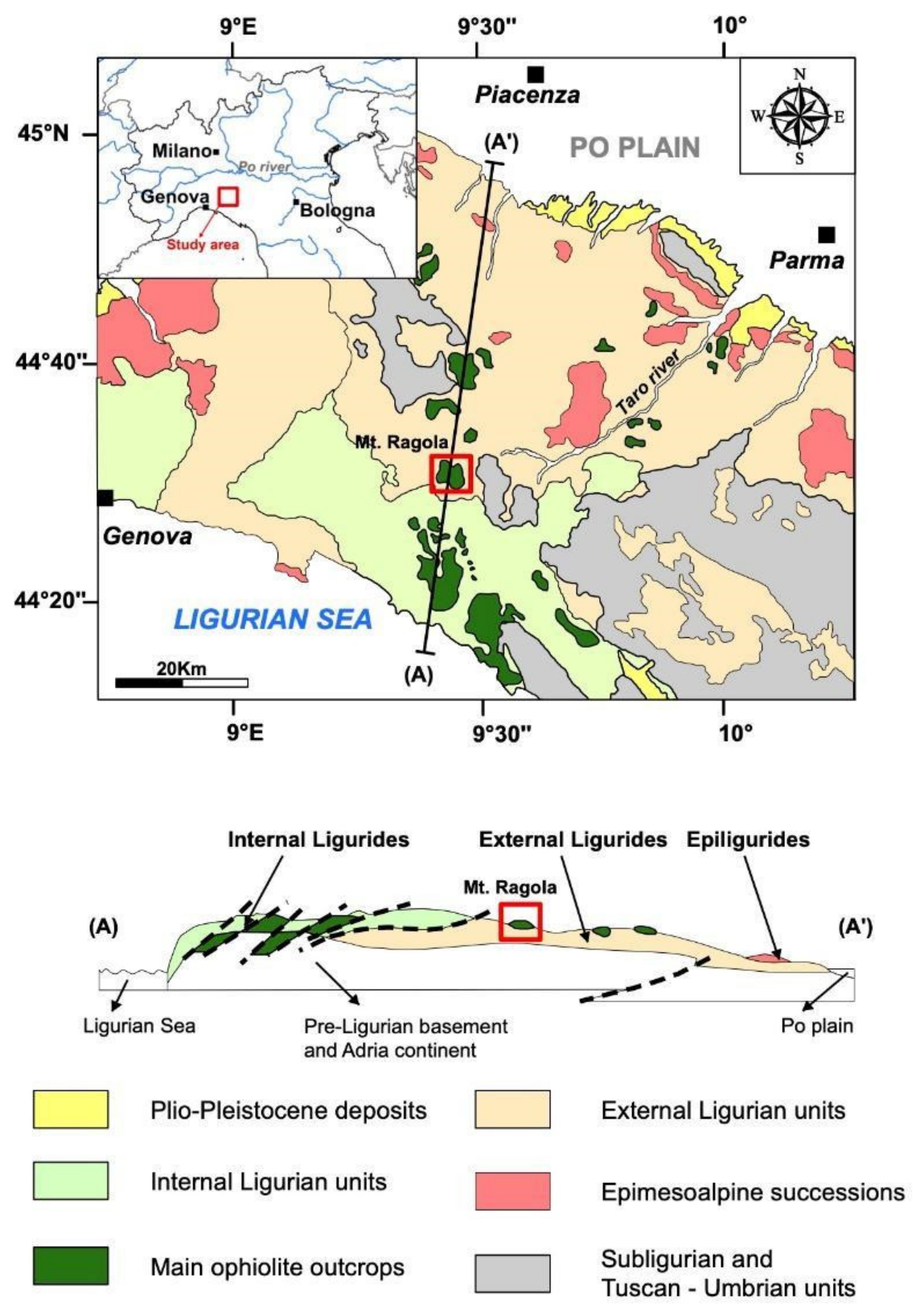
2. General Setting
3. Materials and Methods
- (a)
- Review of the following historical archives acquired by the Geological, Seismic, and Soil Service, reprocessed in GIS environment (georeferenced to the UTM system RER-ED50):
- Color orthophotographs taken on 2006, [17];
- Color orthophotographs taken on 2000, [17];
- Black and white orthophotographs taken between the years 1994 to 1998, [17];
- Black and white orthophotographs taken between the years 1988 to 1989, [17]; http://www.pcn.minambiente.it/viewer/ (accessed on 27 June 2022)
- Color aerial photographs at scale 1:13,000 taken between 1976 and 1978;
- Black and white aerial photographs at scale 1:14,000 taken between 1969 and 1973;
- Grayscale aerial photographs IGMI-GAI at scale 1:33,000, with 50 cm average pixel size, and pictures taken on July 1954 [18]; https://servizimoka.regione.emilia-romagna.it/mokaApp/apps/VIGMIGAI1954_H5/index.html (accessed on 27 June 2022) https://servizimoka.regione.emilia-romagna.it/mokaApp/apps/VIGMIGAI1954_H5/index.html
- Historical aerial photographs acquired by Royal Air Force in Emilia-Romagna (1943–1944) [19];
- Historical topographic maps (1860) of the Kingdom of Italy, called “I.G.M. primo impianto” and “I.G.M. secondo impianto” [18]; https://servizimoka.regione.emilia-romagna.it/mokaApp/apps/CST2H5/index.html (accessed on 27 June 2022) https://servizimoka.regione.emilia-romagna.it/mokaApp/apps/CST2H5/index.html
- Map published by the Military Geographical Institute (I.G.M.) in the 1930s of the last century;
- Historical topographic map of 1853 at scale 1:50,000 [18];
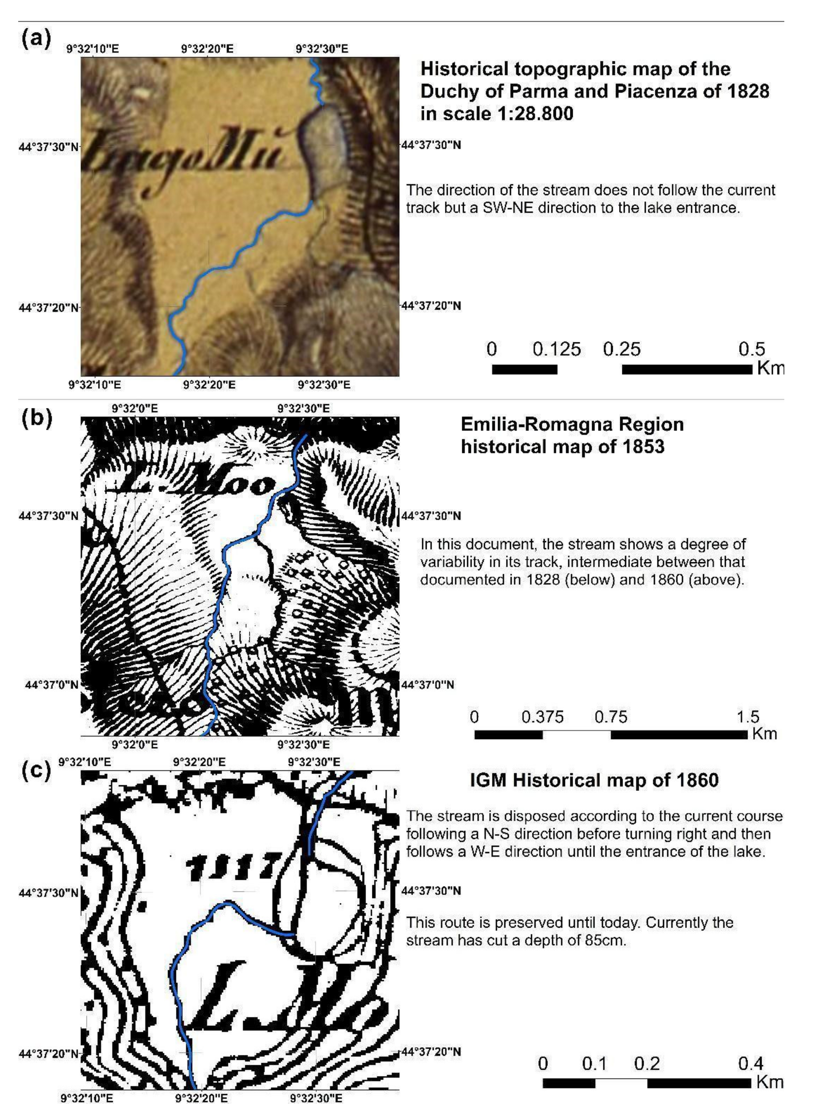
- Historical topographic map of the Duchy of Parma of Piacenza of 1828 at scale 1:28,800 [18]; https://servizimoka.regione.emilia-romagna.it/mokaApp/apps/CST1H5/index.html (accessed on 27 June 2022)
- (b)
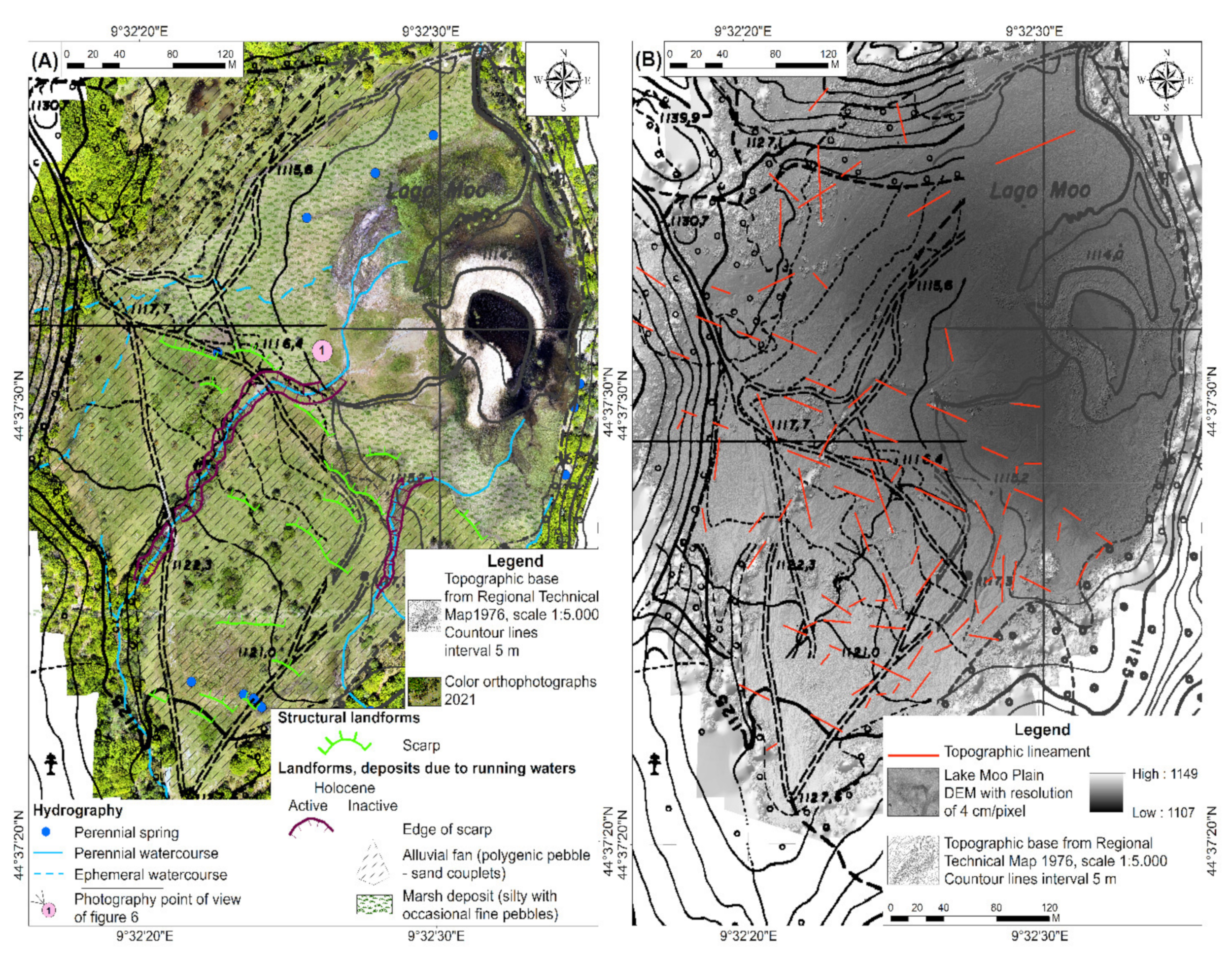
- A new UAV-based photogrammetric acquisition of the entire extension of the Lake Moo basin was performed in Summer 2021 with a 20 MP commercial-grade drone to obtain a 3D model tied to GIS-calibrated ground control points. From this 3D model, we extracted a high-resolution (ca. 1 cm) orthophotograph and DEM used as baseline for detailed mapping of scarps, vegetational/structural and spring alignments, and other geomorphic elements, which were subsequently carefully verified in the field.
- (c)
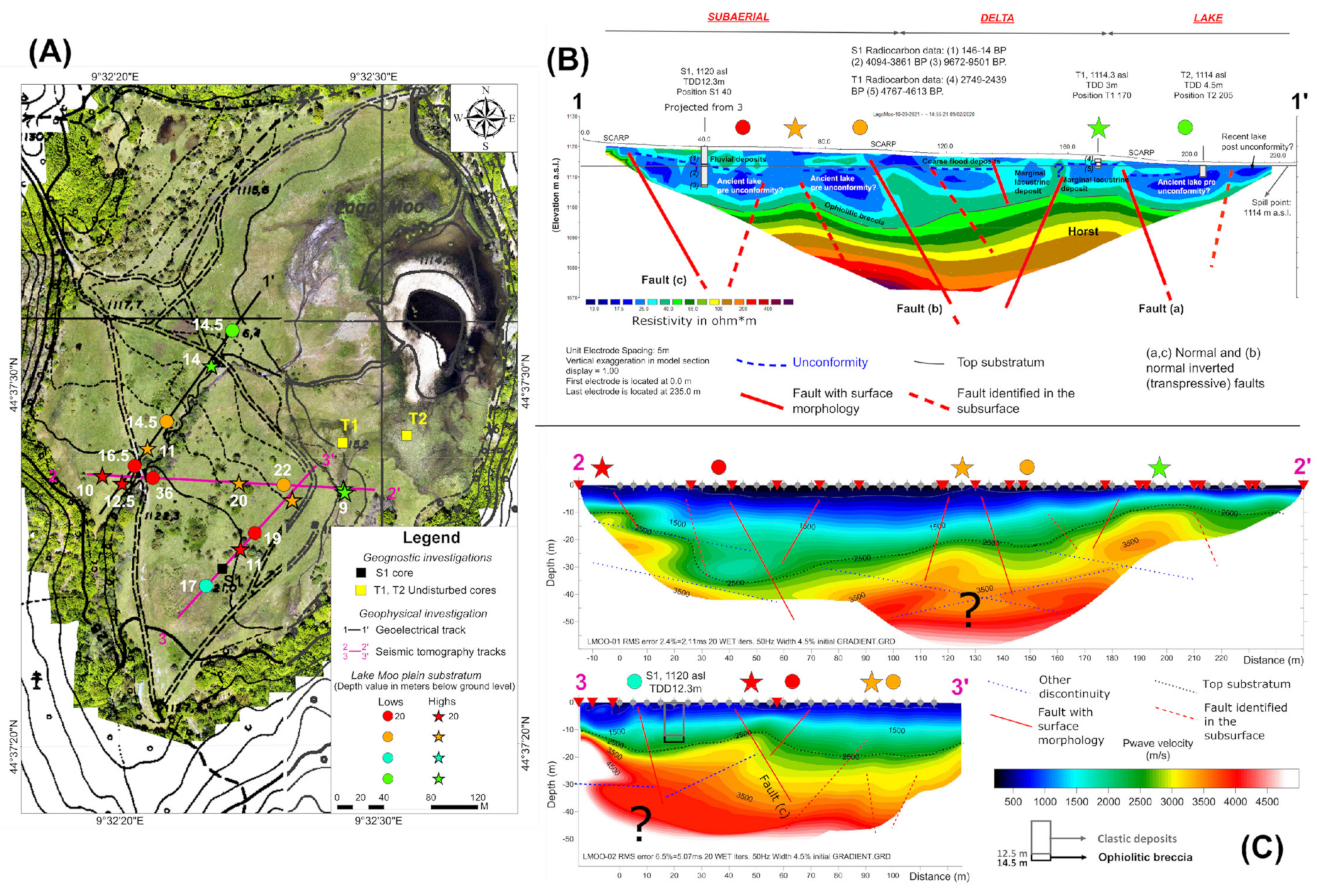
- A geoelectrical survey was carried out in Autumn 2021 to mainly determine the following:
- Depth and geometry of the ophiolite bedrock;
- Location of faults interacting with the bedrock and possibly with the sedimentary cover succession of the lake basin;
- Subsurface depositional trends of sedimentary bodies.
- (d)
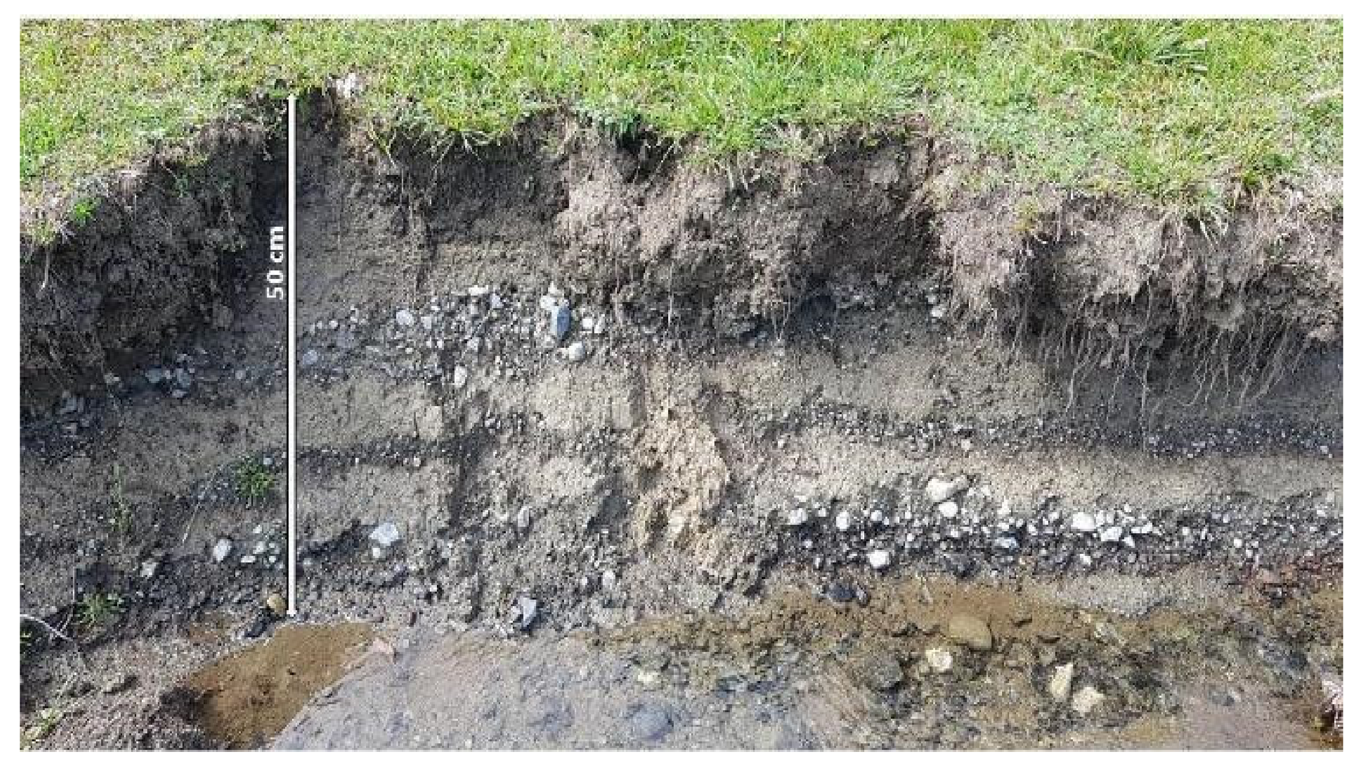
- To investigate the sedimentary succession, two undisturbed sediment cores (T1 and T2) were acquired in summer 2019 in the Lake Moo plain using a Belarus peat corer [21] for a total of 7.5 m (T1, 3 m and T2, 4.5 m) and the lithofacies description is available in Chapter 2 in Supplementary Materials. Complementary data, obtained using a continuous drilling system described in [10] were also used. These data allow us to calibrate the geoelectric measurement data, establishing the resistivity range of various lithological units.
- (e)
- The chronostratigraphic framework was partly based on radiocarbon data from core S1 [10] integrated by two newly acquired radiocarbon ages obtained at the CEDAD Laboratory of the University of Salento (Italy). Original data are available in Chapter 3 in Supplementary Materials.
- (a)
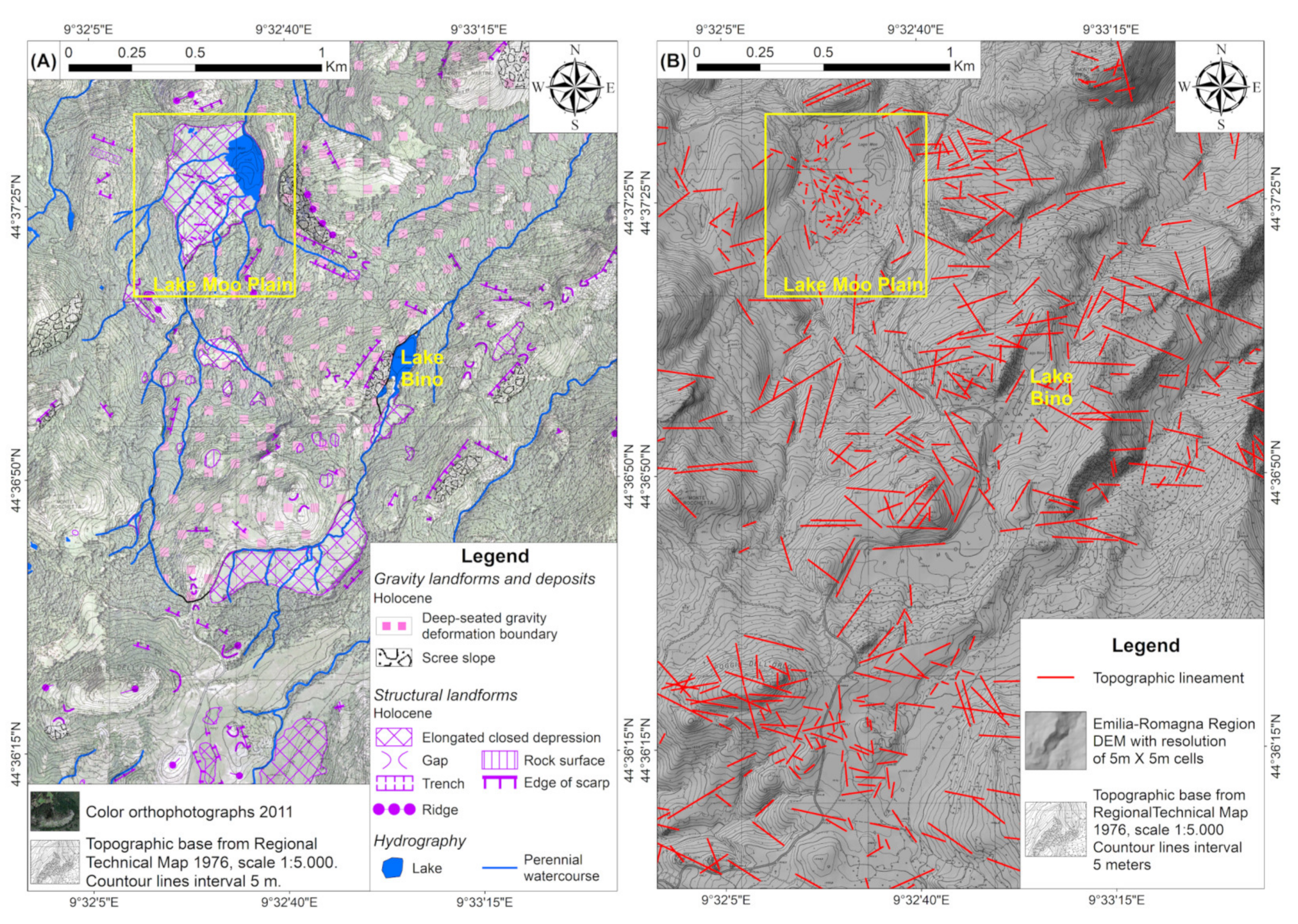
- Orthophotographs and DEM acquired by the Geological, Seismic, and Soil Service, analyzed in GIS environment (georeferenced to the UTM system RER-ED50), in particular, colored orthophotographs A.G.E.A., with a 30–50 cm average pixel size and pictures taken between May and June 2011, and June and August 2008, backed up by high-resolution colored UAV orthophotographs, specifically collected in June 2021. The workflow on DEM involved the outlining of topographic lineations using 4 illumination directions (0–90–180–270), sun position at 45°, and regular time intervals analysis, subsequently backed up by recognition of the same structures on aerial/UAV orthophotographs and directly on site. Saddles, scarps, crests, closed depressions, trenches, terraces, counter slope surfaces, hillbridges, vegetational alignments, and other elements were identified and mapped. The DEM used had a resolution of 5 m × 5 m cells.
- (b)
- Background geological data at the 1:10,000 scale, derived from the Emilia-Romagna Region database [22]. This database was integrated with an original geomorphological survey backed up by photointerpretation, and the results were carefully verified on site. The following complementary datasets and related interpretations from [23] were also used as baseline:
- The morphometry of the hydrographic network, which evidenced a segmentation of the tributaries of the Nure river, interpreted as driven by mechanical discontinuities of the bedrock substrate;
- The meso-tructural analysis on brittle structures (e.g., faults, fractures) in the different lithological units, which highlighted the occurrence of tectonic lineaments and structural trends, interpreted as active also during the Holocene.
- (c)
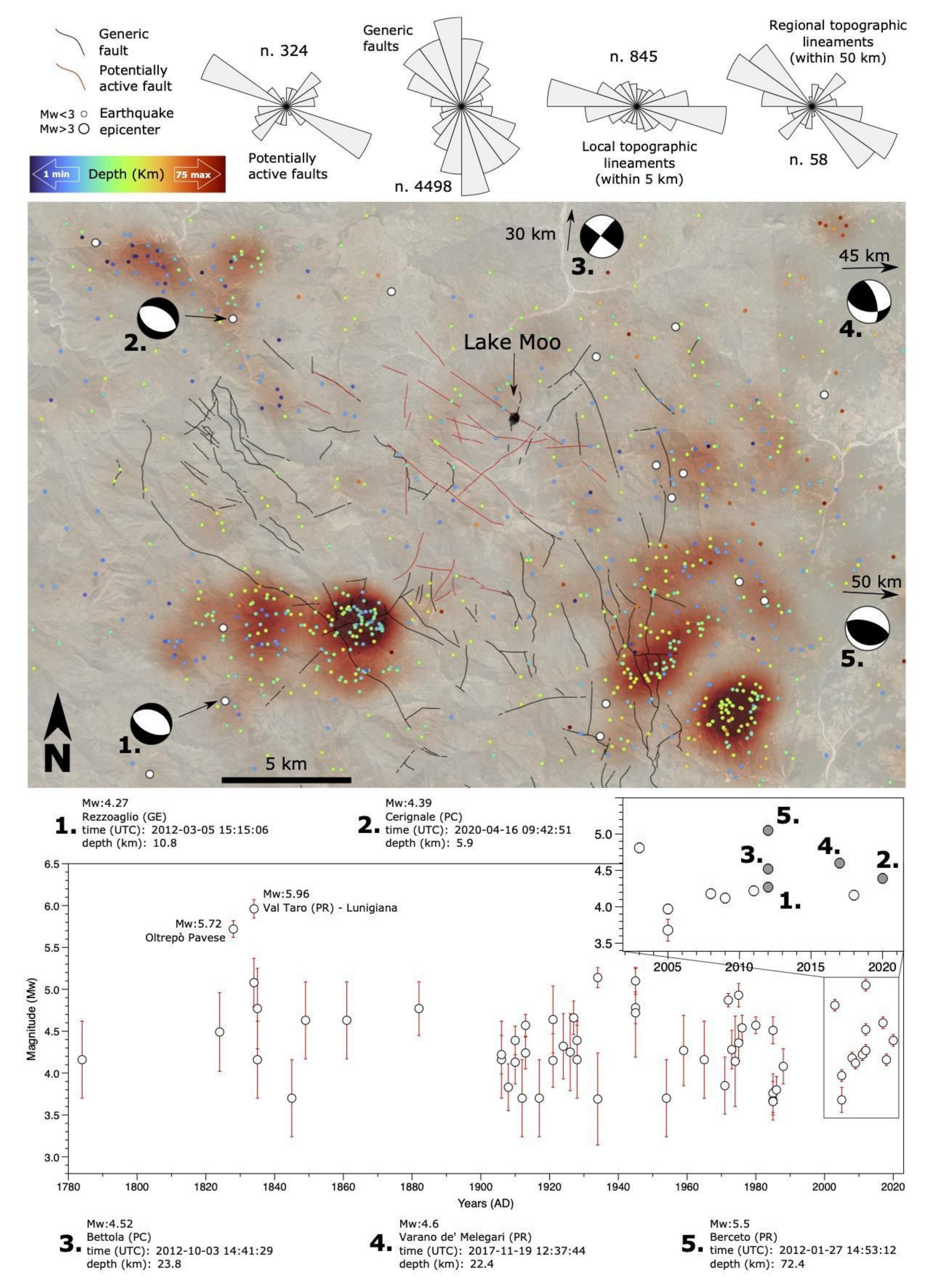
- Finally, we reviewed the national earthquake catalog [24] to qualitatively identify possible relationships between epicentral clustering trends and structural patterns.
4. Data Analysis
4.1. Surface Data
- (a)
- In 1828 (Figure 5a), the main stream feeding Lake Moo was not following the current trend. On the contrary, it appeared to flow on the eastern side of the depression along a NE–SW direction.
- (b)
- In 1853 (Figure 5b), the stream was located in an intermediate position, flowing roughly in the middle of the depression. In 1860 (Figure 5c), the stream had already reached the current configuration in the western part of the basin, along a NW–SE direction that abruptly bent toward the East (with an angle of ca. 90°) before entering into the lake.
4.2. Subsurface Data
4.3. Large-Scale Surface Data
5. Discussion
6. Conclusions
- (1)
- Enhanced efficiency of regular fluvial discharge in humid and cold climatic conditions at the demise of the Little Ice Age;
- (2)
- Deep-seated slope gravity deformation due to tectonic uplift, unroofing, and lateral valley unloading;
- (3)
- Temporal–spatial clustering of seismic events along specific directions parallel to the local to regional structural grain.
Supplementary Materials
Author Contributions
Funding
Acknowledgments
Conflicts of Interest
References
- Elter, P.; Ghiselli, F.; Marroni, M.; Ottria, G. Note Illustrative del Foglio 197 “Bobbio” della Carta Geologica d’Italia alla Scala 1:50.000; Istituto Poligrafico e Zecca dello Stato: Rome, Italy, 1997; pp. 1–106. [Google Scholar]
- Marroni, M.; Meneghini, F.; Pandolfi, L. Anatomy of the Ligure-Piemontese subduction system: Evidence from Late Cretaceous-middle Eocene convergent margin deposits in the Northern Apennines, Italy. Int. Geol. Rev. 2010, 52, 1160–1192. [Google Scholar] [CrossRef]
- Marroni, M.; Meneghini, F.; Pandolfi, L. A revised subduction inception model to explain the Late Cretaceous, double-vergent orogeny in the precollisional western Tethys: Evidence from the Northern Apennines. Tectonics 2017, 36, 2227–2249. [Google Scholar] [CrossRef]
- Molli, G. Northern Apennine-Corsica orogenic system: An updated overview. Geol. Soc. Lond. Spec. Publ. 2008, 298, 413–442. [Google Scholar] [CrossRef]
- Segadelli, S.; Vescovi, P.; Ogata, K.; Chelli, A.; Zanini, A.; Boschetti, T.; Petrella, E.; Toscani, L.; Gargini, A.; Celico, F. A conceptual hydrogeological model of ophiolitic aquifers (serpentinised peridotite): The test example of Mt. Prinzera (Northern Italy). Hydrol. Processes 2016, 32, 969–1201. [Google Scholar] [CrossRef]
- Segadelli, S.; Vescovi, P.; Chelli, A.; Petrella, E.; De Nardo, M.T.; Gargini, A.; Celico, F. Hydrogeological mapping of heterogeneous and multi-layered ophiolitic aquifers (Mountain Prinzera, northern Apennines, Italy). J. Maps 2017, 13, 737–746. [Google Scholar] [CrossRef]
- Segadelli, S.; Filippini, M.; Monti, A.; Celico, F.; Gargini, A. Estimation of recharge in mountain hard-rock aquifers based on discrete spring discharge monitoring during base-flow recession. Hydrogeol. J. 2021, 29, 949–961. [Google Scholar] [CrossRef]
- Chelli, A.; Segadelli, S.; Vescovi, P.; Tellini, C. Large-scale geomorphological mapping as a tool to detect structural features: The case of Mt. Prinzera ophiolite rock mass (Northern Apennines, Italy). J. Maps 2016, 12, 770–776. [Google Scholar] [CrossRef] [Green Version]
- Mariani, G.S.; Zerboni, A. Surface Geomorphological Features of Deep-Seated Gravitational Slope Deformations: A Look to the Role of Lithostructure (N Apennines, Italy). Geosciences 2020, 10, 334. [Google Scholar] [CrossRef]
- Segadelli, S.; Grazzini, F.; Rossi, V.; Aguzzi, M.; Marvelli, S.; Marchesini, M.; Chelli, A.; Francese, R.; De Nardo, M.T.; Nanni, S. Changes in high-intensity precipitation on the northern Apennines (Italy) as revealed by multidisciplinary data over the last 9000 years. Clim. Past 2020, 16, 1547–1564. [Google Scholar] [CrossRef]
- Ghiselli, G.; Marroni, M.; Ottria, G.; Zecca, P. Carta Geologica dell’Appennino Emiliano-Romagnolo 1:10.000, Sezione 197150 Ferriere Est; Regione Emilia-Romagna, SELCA stampe: Florence, Italy, 1999. [Google Scholar]
- Marchetti, G.; Fraccia, R. Carta geomorfologica dell’alta Val Nure, Appennino piacentino. Scala 1:25.000. In Il Paesaggio Fisico dell’Alto Appennino Emiliano, 1st ed.; Carton, A., Panizza, M., Eds.; Grafis Edizioni: Bologna, Italy, 1988; pp. 95–120. [Google Scholar]
- Carton, A.; Panizza, M. Il Paesaggio Fisico dell’Alto Appennino Emiliano, 1st ed.; Grafis Edizioni: Bologna, Italy, 1988; p. 182. [Google Scholar]
- Geological, Soil and Seismic Survey of the Emilia-Romagna Region. Available online: https://geo.regione.emilia-romagna.it/cartografia_sgss/user/viewer.jsp?service=geologia (accessed on 29 March 2022).
- Protected Areas, Natura 2000 Network and Forests. Available online: https://ambiente.regione.emilia-romagna.it/it/parchi-natura2000/rete-natura-2000/siti/it4020008 (accessed on 27 January 2022).
- Geosites and Geological Heritage. Available online: https://geo.regione.emilia-romagna.it/schede/geositi/scheda.jsp?id=2140 (accessed on 21 January 2022).
- Geoportale Nazionale. Available online: http://www.pcn.minambiente.it/viewer/ (accessed on 28 June 2022).
- Servizio Moka Regione Emilia-Romagna. Available online: https://servizimoka.regione.emilia-romagna.it/mokaApp/apps/VIGMIGAI1954_H5/index.html (accessed on 28 June 2022).
- Geoportale Regione Emilia-Romagna. Available online: https://geoportale.regione.emilia-romagna.it/applicazioni-gis/regione-emilia-romagna/cartografia-di-base/cartografia-storica (accessed on 28 June 2022).
- Original High-Resolution Reflection Seismic Data. Available online: https://cp.copernicus.org/articles/16/1547/2020/cp-16-1547-2020-supplement.pdf (accessed on 29 March 2022).
- Jowsey, P.C. An improved peat sampler. New Phytol. 1966, 65, 245–248. [Google Scholar] [CrossRef]
- Geological cartography webgis. Available online: https://ambiente.regione.emilia-romagna.it/en/geologia/cartography/webgis/geological-cartography-webgis?set_language=en (accessed on 29 March 2022).
- Perotti, C.R.; Savazzi, G.; Vercesi, P.L. Evoluzione morfotettonica recente della zona compresa tra la testata del T. Nure e la Val d’Aveto (Appennino piacentino). Suppl. Geogr. Fis. Dinam. Quat. 1988, 1, 121–140. Available online: http://www.glaciologia.it/wp-content/uploads/Supplementi/FullText/SGFDQ_I_1988_FullText/12_SGFDQ_I_1988_Perotti_121_140.pdf (accessed on 27 June 2022).
- Rovida, A.; Locati, M.; Camassi, R.; Lolli, B.; Gasperini, P.; Antonucci, A. (Eds.) Italian Parametric Earthquake Catalogue (CPTI15); Version 4.0; Istituto Nazionale di Geofisica e Vulcanologia (INGV): Rome, Italy, 2022. [Google Scholar] [CrossRef]
- Samartin, S.; Heiri, O.; Joos, F.; Renssen, H.; Franke, J.; Brönnimann, S.; Tinner, W. Warm Mediterranean mid-Holocene summers inferred from fossil midge assemblages. Nat. Geosci. 2017, 10, 207–212. [Google Scholar] [CrossRef]
- Soldati, M.; Borgatti, L.; Cavallin, A.; De Amicis, M.; Frigerio, S.; Giardino, M.; Mortara, G.; Pellegrini, G.B.; Ravazzi, C.; Surian, N.; et al. Geomorphological evolution of slopes and climate changes in northern Italy during the late Quaternary: Spatial and temporal distribution of landslides and landscape sensitivity implications. Geogr. Fis. E Din. Quat. 2006, 29, 165–183. [Google Scholar]
- Brönnimann, S.; Rohr, C.; Stucki, P.; Summermatter, S.; Bandhauer, M.; Barton, Y.; Fischer, A.; Froidevaux, P.; Germann, U.; Grosjean, M.; et al. 1868—L’alluvione che cambiò la Svizzera: Cause, conseguenze e insegnamenti per il futuro. Geogr. Bernensia 2018, 94, 52. [Google Scholar] [CrossRef]
- Giannecchini, R.; D’Amato Avanzi, G. Historical research as a tool in estimating hydrogeological hazard in a typical small alpine-like area: The example of the Versilia River basin (Apuan Alps, Italy). Phys. Chem. Earth 2012, 49, 32–43. [Google Scholar] [CrossRef]
- Stuard Gallery. Available online: https://complessopilotta.it/opera/i-guasti-dellinondazione-di-parma-del-1868/ (accessed on 29 March 2022).
- Bertolini, G.; Pizziolo, M. Risk assessment strategies for the reactivation of earth flows in the Northern Apennines (Italy). Eng. Geol. 2008, 102, 178–192. [Google Scholar] [CrossRef]
- Le Roux, L.; Schwartz, S.; Gamond, J.F.; Jongmans, D.; Bourles, D.; Braucher, R.; Mahaney, W.; Carcaillet, J.; Leanni, L. CRE dating on the head scarp of a major landslide (Séchilienne, French Alps), age constraints on Holocene kinematics. Earth Plan. Sci. Lett. 2009, 280, 236–245. [Google Scholar] [CrossRef]
- Barbano, D.; Perotti, C.; Vercesi, P.L. La tettonica recente dell’alta Val Nure (PC). Atti Ist. Geol. Univ. Pavia 1984, 30, 221–233. [Google Scholar]

Publisher’s Note: MDPI stays neutral with regard to jurisdictional claims in published maps and institutional affiliations. |
© 2022 by the authors. Licensee MDPI, Basel, Switzerland. This article is an open access article distributed under the terms and conditions of the Creative Commons Attribution (CC BY) license (https://creativecommons.org/licenses/by/4.0/).
Share and Cite
Segadelli, S.; Ogata, K.; Cocuccioni, M.; Gambini, S.; Martelli, L.; Morandi, L.F.; Oppo, G. Holocene Evolution of Minor Mountain Lacustrine Basins in the Northern Apennines, Italy: The Lake Moo Case Study. Geosciences 2022, 12, 272. https://doi.org/10.3390/geosciences12070272
Segadelli S, Ogata K, Cocuccioni M, Gambini S, Martelli L, Morandi LF, Oppo G. Holocene Evolution of Minor Mountain Lacustrine Basins in the Northern Apennines, Italy: The Lake Moo Case Study. Geosciences. 2022; 12(7):272. https://doi.org/10.3390/geosciences12070272
Chicago/Turabian StyleSegadelli, Stefano, Kei Ogata, Marco Cocuccioni, Stefano Gambini, Luca Martelli, Lionello F. Morandi, and Gabriele Oppo. 2022. "Holocene Evolution of Minor Mountain Lacustrine Basins in the Northern Apennines, Italy: The Lake Moo Case Study" Geosciences 12, no. 7: 272. https://doi.org/10.3390/geosciences12070272
APA StyleSegadelli, S., Ogata, K., Cocuccioni, M., Gambini, S., Martelli, L., Morandi, L. F., & Oppo, G. (2022). Holocene Evolution of Minor Mountain Lacustrine Basins in the Northern Apennines, Italy: The Lake Moo Case Study. Geosciences, 12(7), 272. https://doi.org/10.3390/geosciences12070272