Kinematic and Geometric Characterization of the Vögelsberg Rockslide (Tyrol, Austria) by Means of MT-InSAR Data

Abstract

This paper focuses on the study of the Vögelsberg landslide located in the municipality of Wattens (Tyrol, Austria), which reactivated in 2016, causing damages to nearby buildings and infrastructures. Since the date of reactivation, a modern monitoring system has been implemented with the installation of in-situ geodetic automated tracking total stations (ATTS), an inclinometer and two piezometers. Here, we describe two distinctive methods, the Breaks for Additive Seasonal and Trend (BFAST) and the Vector Inclination Method (VIM) used to characterize the landslide from the kinematic and geometrical point of view. The main input data, used for both methods, derive from processing a stack of several Sentinel-1 differential interferograms with the Multiple Small Baseline Subset (MSBAS) 2D and 3D algorithms. BFAST allowed highlighting the seasonality of the phenomenon from the analysis of the time series as well as the trend and the breakpoints that identify the landslide reactivation phases. These latter were then correlated with the main triggering factors such as rain and snow melting. The application of the VIM through the exploitation of the MSBAS displacement vectors allowed the reconstruction of the depth of the landslide slip surface along both the longitudinal and transversal direction and, in turn, the evaluation of the volumes of material mobilized by the landslide. The results obtained further prove that procedures for the in-depth analysis of Multi-Temporal Interferometric Synthetic Aperture Radar (MT-InSAR) data can contribute to slow-moving landslide characterization, which represents a fundamental step for landslide hazard assessment within quantitative risk analyses.

1. Introduction

Deep-seated gravitational slope deformations (DSGSDs) are common phenomena in high mountainous regions, especially in deeply incised Alpine valleys. The formation processes and the temporal and spatial evolution of these rock slope instabilities is mainly controlled by predisposing factors such as topography, lithology, geological structures, discontinuity network, geomechanical rock mass properties, in-situ stresses, groundwater flow, valley glacier retreat, permafrost degradation, and temperature fluctuations [1].

As for the kinematic, DSGSDs (here a deep-seated rockslide) are characterized by the downslope movement of a rock mass along one or several rupture surfaces or within a relatively narrow zone of intense shear strain [2]. These slope instabilities can reach thicknesses of tens to hundreds of meters [3,4,5]. According to [6], the rupture surface of rock compound slides consists of an uneven curvature and/or several planes. Internal deformation promotes intact rock bridges to fail and sequential fracture linkage, i.e., progressive failure mechanism; this is necessary to form a fully persistent rupture surface or shear zone to provoke the rock mass into a sliding motion [6,7,8,9,10]. Several case studies, showing bi-linear, stepped, or curved geometries of the basal shear zone are presented in the literature, and a geomechanical relationship is established between deformations in the subsurface and the geomorphological features on the surface [5,6,11,12,13]. The deformation behavior of deep-seated rockslides, as well as the geomechanical behavior and processes that cause fracturing, fragmentation, and internal rock mass deformation, are still not fully understood [14,15].

The knowledge of DSGSD evolution in time requires a better understanding of long-term internal kinematic history and a good knowledge of the deep geometry characteristics of the unstable slope.

MT-InSAR data can be suited for the study of internal kinematics by taking into account its time series; on the other hand, the velocity measurements can be used as a superficial proxy for the interpretation of its more complex geomorphology.

The application of the MSBAS method [16] to multi-temporal high resolution SAR data can deliver 2D (East-West and Up-Down decomposed) [17] and 3D displacement [18] vectors, which can help in landslide sliding surface (LSS) reconstruction by adopting the VIM [19].

Previous findings concerning the hydrological drivers at Vögelsberg were published by [20]. The authors used hydro-meteorological inputs such as precipitation, snow depth, temperature, humidity, wind speed, and global radiation from 13 different weather stations in the surrounding area to feed AMUNDSEN (Alpine MUltiscale Numerical Distributed Simulation ENgine). This model can simulate the water availability for infiltration (which corresponds to rainfall and snowmelt minus evapotranspiration) at the catchment scale. They finally correlated the results of this model to the averaged sum of the horizontal time series displacement (expressed as deformation rate in cm/y) of 14 reflector points linked to an automated geodetic tracking total station (ATTS) at Vögelsberg.

In this paper, the BFAST [21] is applied to MT-InSAR time series data decomposed in the North, East, and Up directions for the first time. This method allowed for the identification of the reactivation phases of the Vögelsberg landslide as highlighted by [20]. The results of BFAST for MSBAS were correlated with the ATTS trends as well. Moreover, by applying the VIM method to the MSBAS velocity measurements, the approximate 3D model of the sliding surface was drawn, and its volume of earth and rock mobilized estimated.

2. Study Site

The Vögelsberg DSGSD is situated on a northeast-facing slope at the lower Watten valley in Tyrol, Austria (Figure 1a). The DSGSD system covers an area of approximately 4.6 km² and ranges from 750 m a.s.l. at the valley bottom to the double-crested mountain ridge at elevations of 1200 m a.s.l. in the north and 2200 m a.s.l. in the south. The study area corresponds to the currently active and slowly moving rockslide (approx. 0.2 km²) embedded in the lower sector of the DSGSD (Figure 1), with temporally varying displacement rates that caused several damages to infrastructure and houses. In a long-term perspective, continuous movements in the range of several centimeters per year may cause a steepening of the slope toe, thus increasing the risk of sudden slope collapse and, in turn, potentially damming of the underlying Watten River.

Lithologies favouring prevailing slope deformation processes belong to the Innsbrucker Quartzphyllite complex of the central Eastern Alps [22]. Sericite phyllites, chlorite-sericite phyllites, and quartz phyllites with intercalated calcareous marbles are apparent on the investigated slope. Greenschist (prasinites) are exposed around the summit of the Largoz, which is the highest point in the DSGSD catchment [23].

The field surveys and in-situ investigations have revealed the presence of two landslide slabs, a north-western (slab A) and a south-eastern slab (slab B) (Figure 1b).

3. Materials and Methods

3.1. Materials

Since spring 2016, the Vögelsberg rock slide (Figure 1b) has been monitored with an automatic tracking total station (ATTS) operated by the Tyrolean state government. The ATTS provides enough temporal resolution and spatial accuracy for assessing the temporal behaviour of the landslide’s movement.

Core drillings on the actively creeping slabs record a shallow quaternary cover above strongly disintegrated quartz phyllite fragments dominated by clay, silt, sand, and gravel grain sizes up to depths of 52–70 m below the surface indicating a long and intense history of deformation. This sequence of unconsolidated rock is assumed to represent the landslide depth where inclinometer measurements indicate distinct displacements between 43 and 51 m below the surface [23].

3.1.1. Ancillary Data

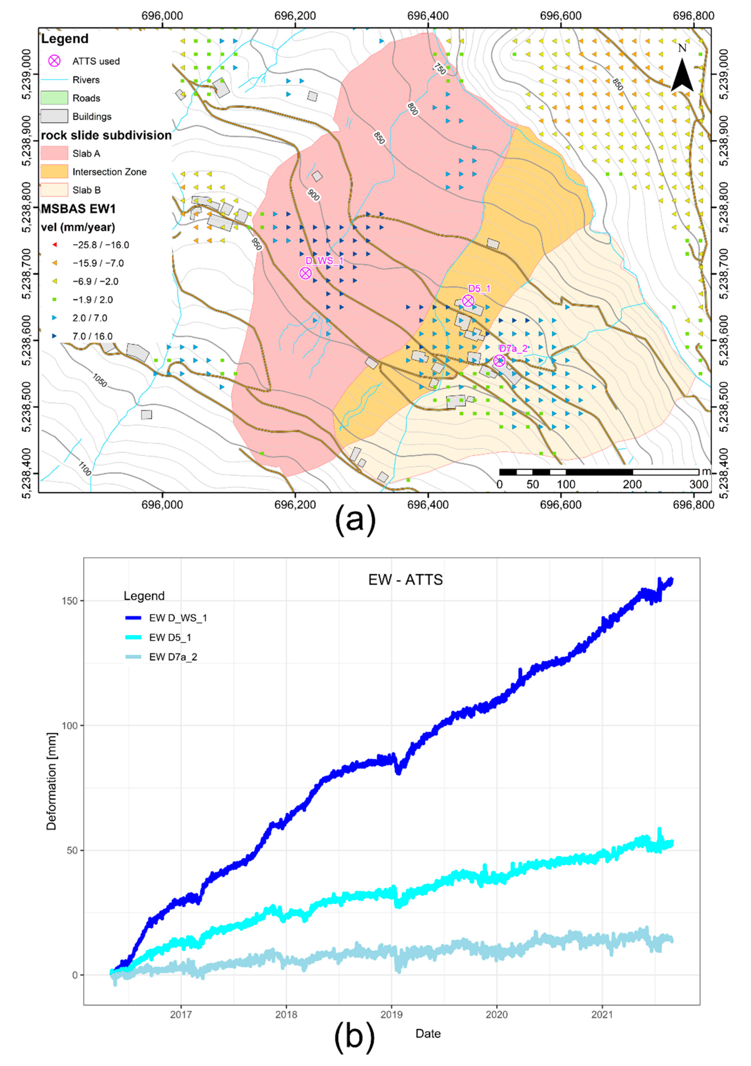
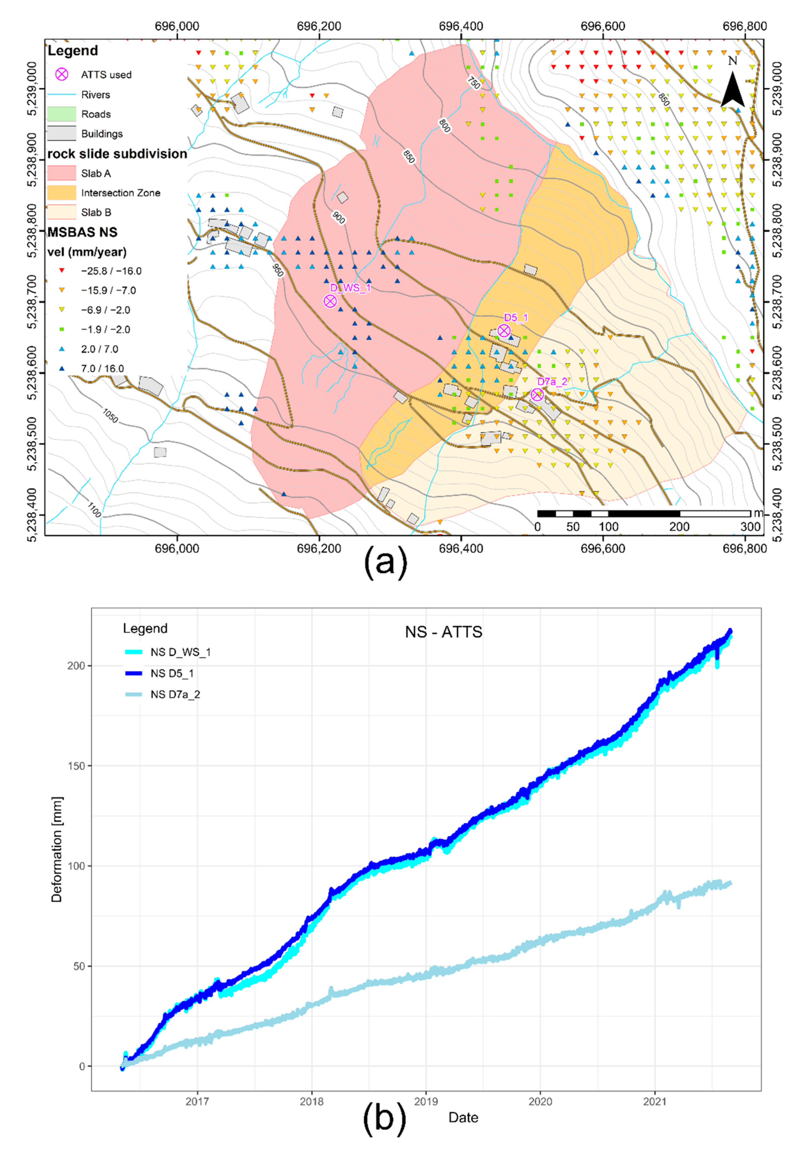
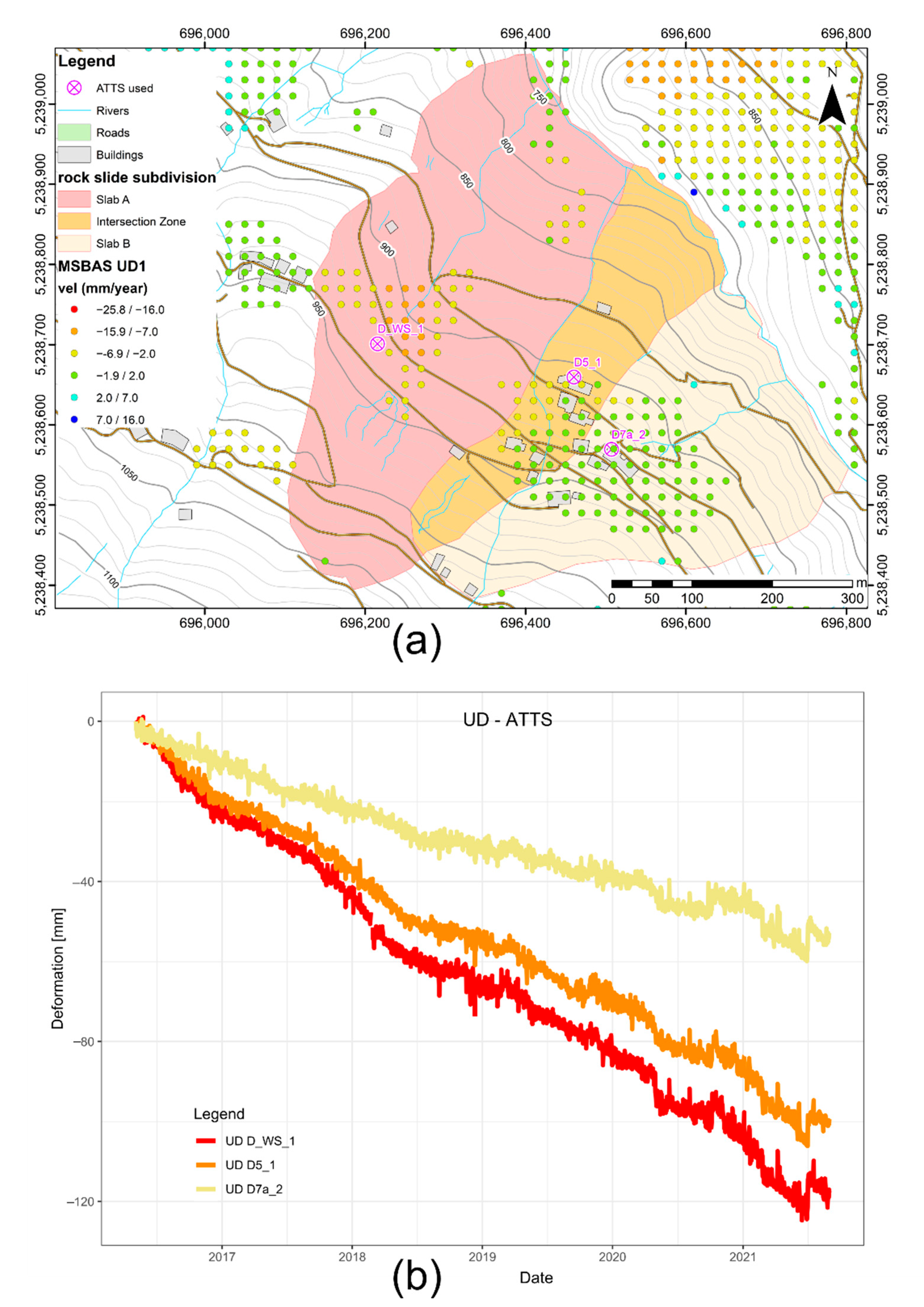
For this study, three ATTS reference points (D5_1, D_7a2, D_WS_1) (Figure 1b) were used. Those three points allowed inspecting the major trend of motion because each point is representative of the style of motion of each individual slab. From 2016 to 2021, for each point, cumulative vertical and horizontal displacements are reported as follows:

• Slab A: 27.6 cm of horizontal displacement and −11.6 cm of vertical displacement.
• Intersection zone: 22.4 cm horizontal displacement and −10 cm vertical displacement.
• Slab B: 9.2 cm horizontal displacement and −5.2 cm vertical displacement.

The weather station (courtesy of Institute of Meteorology and Geodynamic ZAMG) used for the evaluation of precipitation and snow depth is “Jenbach” (530 m a.s.l.), located approximately 14 km northwest of the active landslide. At Jenbach, between 2010 and 2020, a mean annual precipitation of 1223 mm was registered.

Mainly precipitation and snow depth data were used in the present study; more in detail, daily, and weekly cumulative rainfall and the total cumulative precipitation from 2016 to October 2021 were calculated. This was the basis for the time series and trend analysis described in the following chapters.

Data of three core drillings conducted within the active landslide body (owned by the municipality of Wattens and analyzed by the Torrent and Avalanches Control-WLV), two of them equipped with piezometers (KB1, KB2) and the third with an inclinometer (KB3) (Figure 1b), were available. These latter were used as reference points in the reconstruction of the landslide 3D model.

After [24], a summary classification of damage severity levels affecting the buildings was made. In particular, three damage levels were identified:

• Low damage (green): less visible outside wall cracks; easily eliminated with normal painting works.
• Medium damage (yellow): clearly visible outside wall cracks. It may be necessary to refurbish limited masonry components; locked doors and windows.
• High damage (red): restoration works required, with partial or total removal of the artefact; danger of collapse.

Most of the eight highlighted buildings in Figure 1b show similar damage severity levels as new cracks with different extensions and thicknesses on the exterior façade as well as on the interior, detachments in different parts of the structures, and shifting and tilting effects.

The AMUNDSEN model applied to the Vögelsberg landslide by [20] provided a further source of information in this work. Considering a 10-day cumulative rainfall over the period from 2 September 2015 to 14 June 2019, the model identified three major hydro-meteorological events (

Table 1. Summary of the main acceleration events over Vögelsberg rockslide in the period 2016–2019 according to [20,23].

Event	Period	Main Trigger Factor	Source
1	August 2016	snow and rainfall	Pfeiffer et al., 2020 [21]
2	June 2017–February 2018	rainfall	Pfeiffer et al., 2020 [21]
2.b	September 2017–April 2018	snow and rainfall	Engl, 2018 [24]
3	March 2019–April 2019	snow melting	Pfeiffer et al., 2020 [21]

) causing landslide acceleration, which can be summarized as follows:

• Event 1: connected to a maximum horizontal displacement rate of 5.71 cm/year and a reactivation phase in August 2016; this event is rain- and snowmelt-dominated and it has a delay-response time varying in the range of 20–60 days.
• Event 2: connected to a second acceleration phase starting in mid-July 2017 and reaching its maximum displacement rate equal to 4.98 cm/year in February 2018; this event is rainfall-dominated and has a delay-response time of 45 days.
• Event 3: connected to a third acceleration phase recorded in March and April 2019 with maximum displacement rate of 3.57 cm/year; this event is mainly snowmelt- dominated and has a delay-response time of 8 days.

Ref. [23] highlighted the presence of an additional event in the period between September 2017 and April 2018 that approximately overlaps the second event (Event 2.b in Table 1).

The approach proposed by [20] differs from the one introduced by [23], since the latter analyzes the horizontal displacement (expressed as deformation rate in cm/year) only for the quickest part of the landslide on Slab A (Figure 1b), exemplified by the station number D_WS_1.

3.1.2. Newly Acquired Data

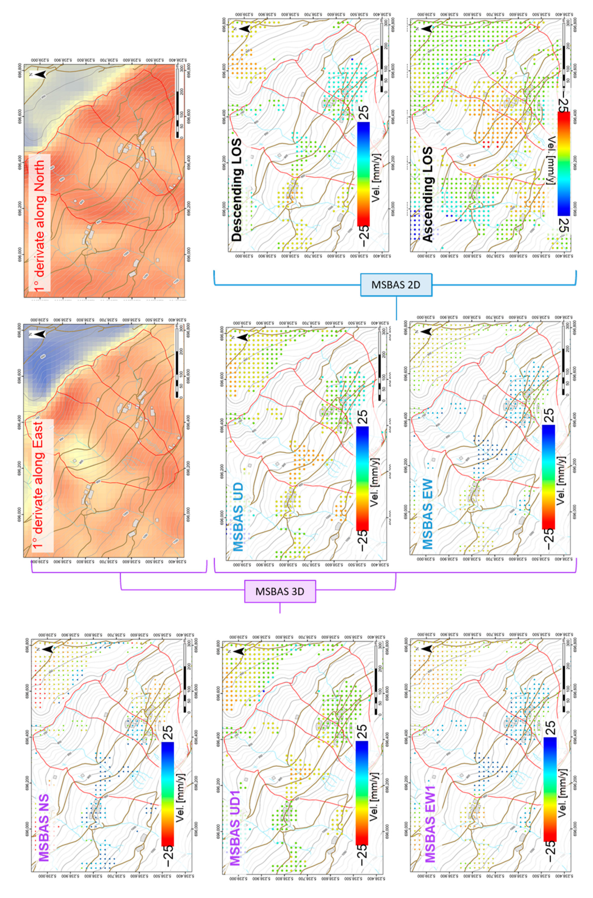
The Multidimensional Small Baseline Subset (MSBAS) methodology is developed for simultaneous post processing of hundreds to thousands of individual interferograms produced by a conventional DInSAR processing [17,18].

For the conventional DInSAR processing, in this paper, the “InSAR automated Mass processing Toolbox for multidimensional Time series” (MasTer) [25] has been used; this software supports the MSBAS method for the creation of the SBAS-based time series in ascending, descending, and combined mode. The MSBAS 2D method allows the extraction of the east (V_E) and vertical (V_V) components from the sensor-target line of sight (V_LOS) and deformation vectors obtained in ascending and descending acquisition geometries.

However, for gravity-driven phenomena such as landslides, the North-South component is non-negligible; that is why the MSBAS problem for computing North, East, and vertical velocities requires information from three different DInSAR acquisition geometries to be solved. In order to obtain the North component from the MSBAS 2D results (V_E and V_V), the following equation can be applied:

$$V_V=\frac{\partial H}{\partial X_N} V_N+\frac{\partial H}{\partial X_E} V_E$$

(1)

where H is the topographic height, ∂H/(∂X_N) and ∂H/(∂X_E) are first derivatives of H in the North X_N and East X_E directions. The ∂H/(∂X_N) and ∂H/(∂X_E) can be computed from the available DEM. The 3D components are calculated thanks to application of the Singular Value Decomposition (SVD) method and a numerical integration, which allows obtaining the 3D time series of displacements for each pixel. In Figure 2, the workflow for the used MSBAS 3D algorithm is shown. Furthermore, in Figure 3, Figure 4 and Figure 5, the results of the MSBAS 3D is shown alongside the time series for the reference ATTS stations.

In the present case study, 184 Sentinel-1 images from the ascending track n. 117, which formed a network of 1088 interferograms and 209 images for the descending track n. 95 and a network of 1578 interferograms, were used as input data for the MSBAS 2D and 3D algorithms. For both datasets, the acquisition dates spanned between May 2016 and October 2021.

3.2. Methods

The methodology adopted in this paper consists of four main phases as shown in Figure 6.

As for the kinematic characterization, the BFAST method was applied for the first time to a landslide study (Phase 1) for the decomposition and linearization of an MT-InSAR time series derived by the MSBAS 2D and 3D input data. The results obtained were then cross-compared in Phase 2 with the displacement data recorded by an in-situ ATTS system and the available landslide triggering information.

On the other hand, the MSBAS 2D and 3D datasets were used to reconstruct the 2D (Phase 3) and 3D (Phase 4) landslide-sliding surface by applying the Vector Inclination Method (VIM) for the geometric characterization of the analysed landslide.

3.2.1. MT-InSAR Time Series Decomposition with BFAST

An MT-InSAR derived time series can provide consistent measurements of ground deformation. Since every pixel of a processed MT-InSAR is associated with a time series information, it is not an easy task to check differences and common patterns between close pixels in terms of temporal evolution.

In this case, change detection methods can be used for the detection of distinct moments in time when:

• seasonal changes driven by annual climate variability occur;
• gradual changes such as inter-annual climate variability (e.g., trends in mean annual rainfall) occur;
• abrupt changes, caused by the interaction of long-time and intense precipitation and snow melting that could control ground instabilities activity, are taking place [26];
• extra triggering events are present.

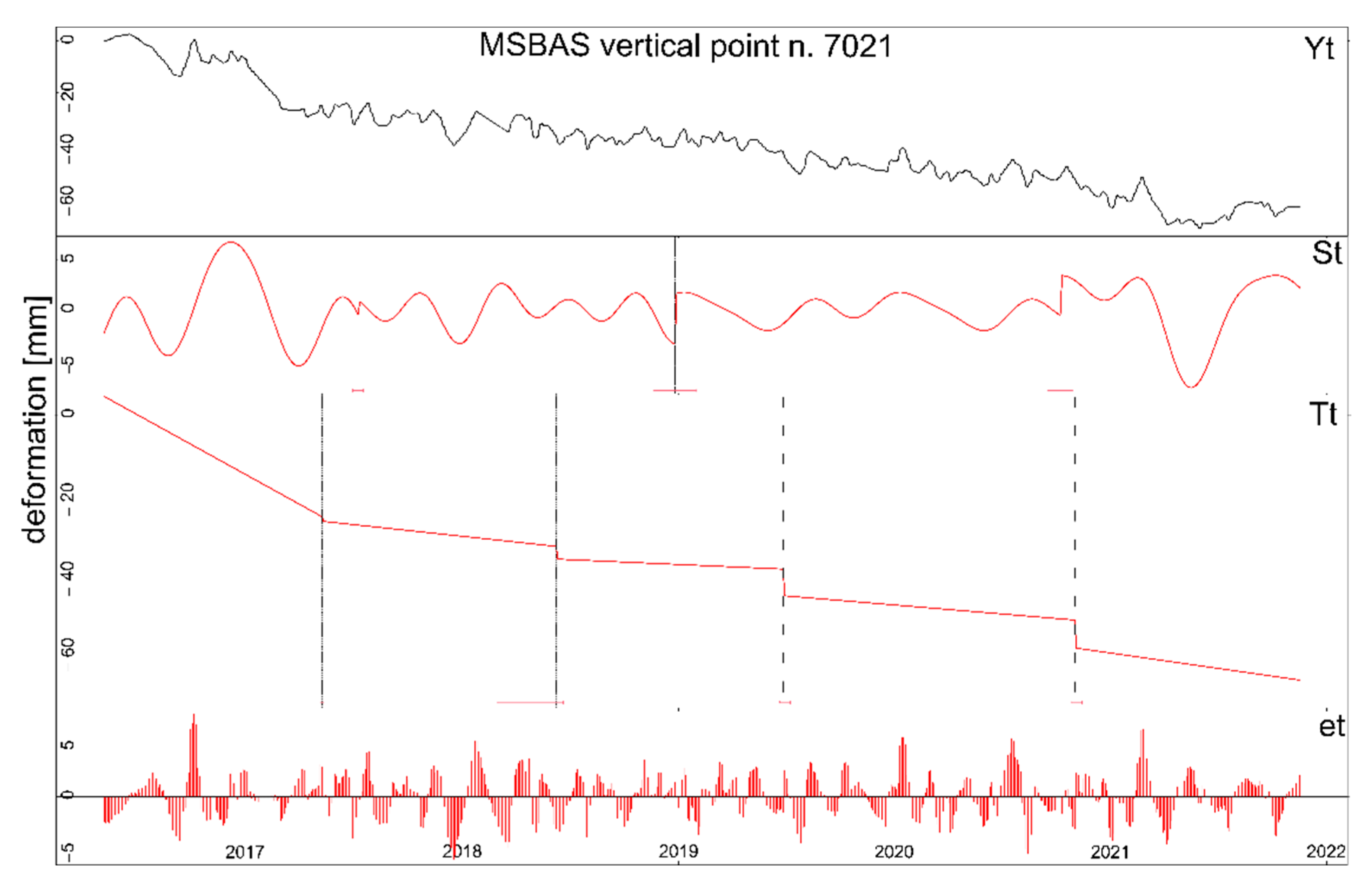
Even though the classical Seasonal-Trend decomposition using the LOESS (STL) algorithm is capable of separating the trend and seasonal component, the STL applies a smoothing factor that obliterates the change [21]. BFAST is a time series change detection algorithm able to detect multiple breakpoints within a time series. It decomposes at first the original data Yt into trend (Tt), seasonal (St), and error (et) components (Figure 7) using Seasonal decomposition of Time series by Loess (STL) [27]. On those two separated components, an ordinary least-squares residual moving sum (OLS-MOSUM) test is performed in order to evaluate the existence of at least a break point. If this is the case, a univariate piecewise regression line is fitted to identify the location of the breaks in the trend and in the seasonal. BFAST uses the intercept and slope of consecutive piecewise lines to estimate magnitude and direction of change. Piecewise linear models are often used to highlight basic features from complex data [26].

The BFAST method has the advantage to be open source since it is compiled in R language; a minor disadvantage lies in the fact that in order to be applied to a time series of regular evenly spaced observations, the dataset must not contain empty values. To overcome this problem, a linear interpolation (imputing) algorithm can be applied in order to fill up the empty values present in the original dataset.

The BFAST approach has been worldwide used for different applications [28,29,30,31,32]. A very similar approach was used by [33], who carried out the signal decomposition of PSI InSAR measurements by means of piecewise linear deformation for the detection of building and infrastructure instability in Beijing.

3.2.2. Two- and Three-dimensional Landslide Geometry Reconstruction by Applying the VIM Method

The shape and depth of a LSS [19] can be outlined from the distribution and magnitude of surface displacement (both vertical and horizontal).

In this regard, a simplified approach based on a geometric technique is the vector inclination method (VIM) that allows delineating both the geometry and depth of a sliding surface when enough displacement information on the landslide ground surface is available.

The VIM method, proposed by [34,35], relies on three main assumptions:

• a single slide surface exists,
• the landslide mass moves as a rigid body,
• a point on the ground will move in a direction that is parallel to the sliding surface beneath.

These hypotheses are appropriate for planar and circular slips, where the slope moves as a solid body, but are hardly suitable for other shapes of slip surface or where high ground deformations occurs within the landslide body [34].

In order to use this method, the displacement monitoring points must be available closely to the work section, and the measurement points (MPs) should be re-projected on the section along the shortest distance. First, the EW displacement component is projected along the selected section planes by means of simple trigonometric formulas, considering that the maximum displacement is expected on the planes containing the steepest slope directions and these can be approximated to the section planes [19].

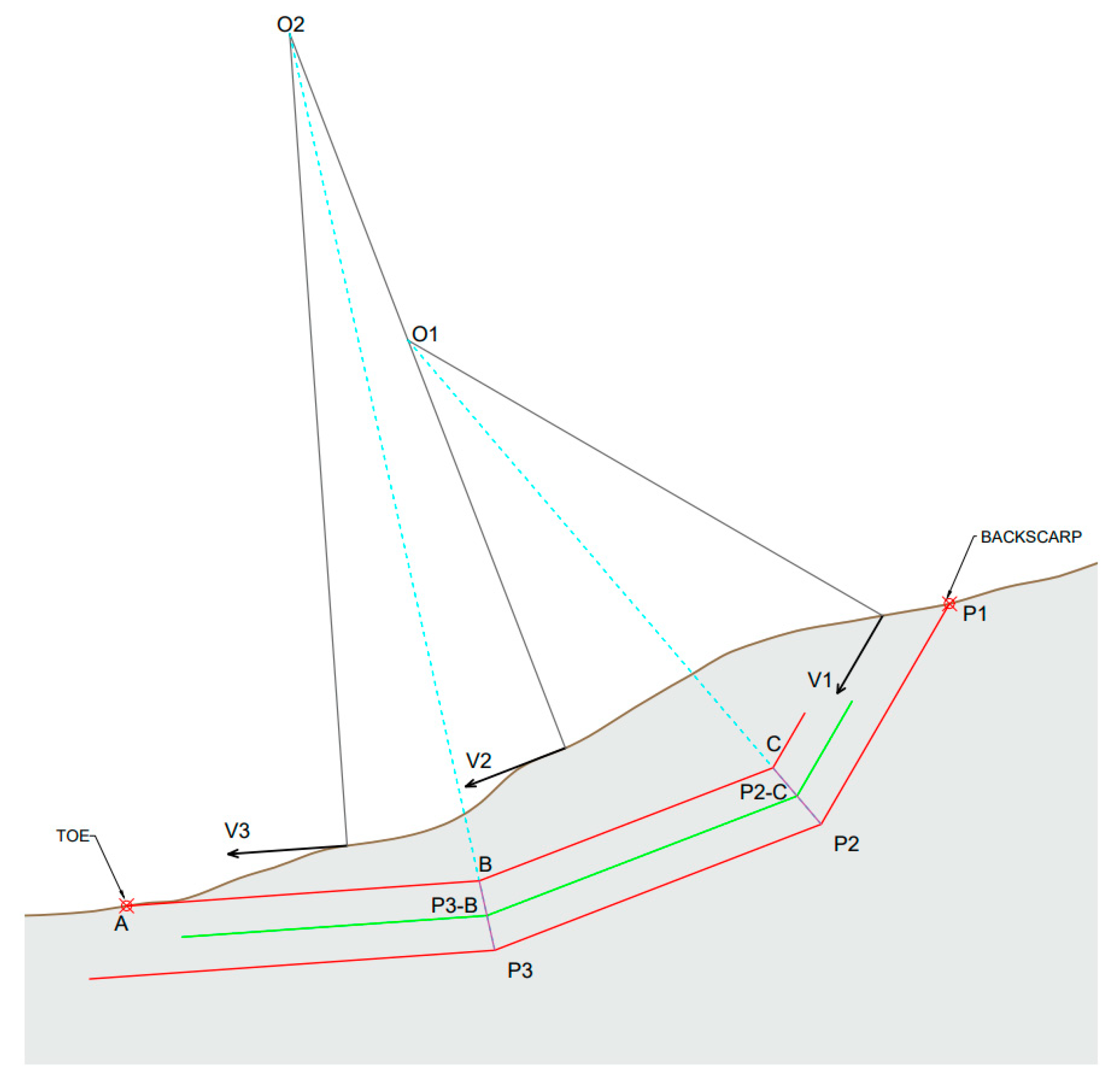
By looking at Figure 8, the normal (in black) to the available vectors (V1, V2, V3) was drawn and once found, the intersection (O1, O2) between two consecutive normal lines and the bisection lines (cyan) is projected. Then, a parallel line to the first vector, starting from the back scarp of the landslide (point P1) up to the intersection (P2) with the first bisection line, was drawn. A second parallel line to the second vector (V2) from P2 to P3 is created. This procedure must be repeated for each available movement vector and in both ways (from back scarp to toe and vice versa).

Based on above consideration and considering the position of the boreholes KB2 and KB1 as well as the inclinometer KB3 (Figure 1b), the VIM method was applied to the studied landslide along two section profiles (A-A’ and B-B’, Figure 1b) with the aim of drawing the LSS along the steepest slope. This choice allowed fixing points for direct validation of the results and a comparison with the landslide model proposed by [23].

As an absolute novelty, the application of the VIM method was also attempted along the cross sections of the landslide on directions roughly oriented orthogonally to the A-A’ and B-B’ sections. This was possible thanks to the displacement information derived by the application of the MSBAS 3D algorithm, which provides the deformation velocity for each pixel in 3D directions (i.e., vertical, north, and east). For the cross sections C-C’ and D-D’ (Figure 1b), the North-South and Up-Down components were considered to reconstruct the LSS depth and shape.

4. Results

According to the methodology adopted (Figure 6), first the BFAST method was applied to the MSBAS data (Figure 3) in EW, UD, EW1, UD1, and NS directions. Overall, 173 points were considered for each direction, which amounts to 865 time series analysed. Then, the ATTS reflectors (D5_1, D_7a2, D_WS_1) in the three movement directions were treated with the BFAST and compared with the MSBAS data.

From the application of the BFAST method, it was possible to identify trends in the time series (TSs), which present two, three, or four break points (BPs) occurring in recurrent intervals and with equal or different magnitude. Furthermore, the BFAST provides a 95% confidence interval error bar for each BP detected.

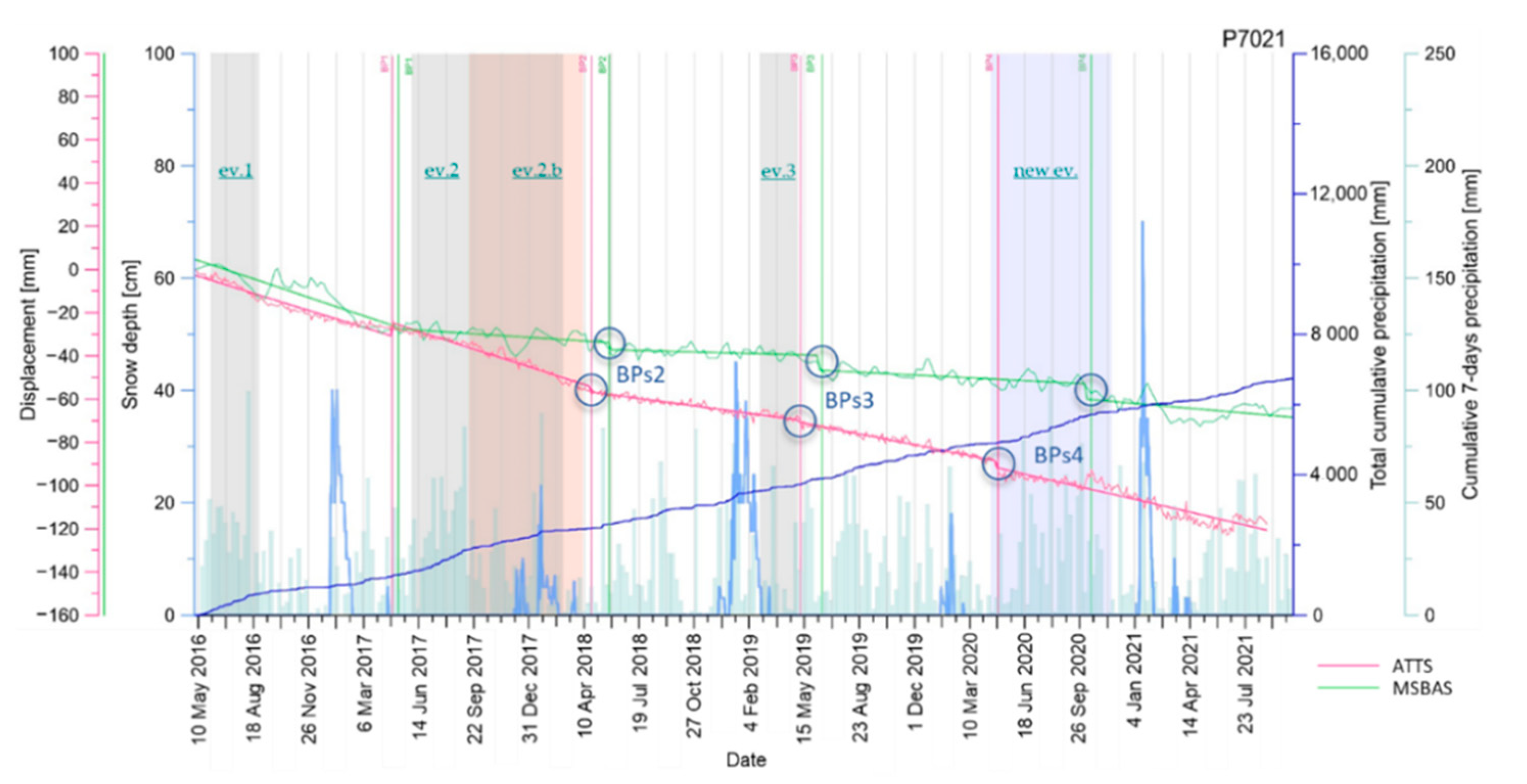
The total cumulative precipitation, cumulative 7-day precipitation, and the snow depth have been plotted against the displacements of the ATTS taken as a reference and compared with the displacements of the MSBAS points.

For the comparison, only the MSBAS points that showed spatial proximity and similar distribution of BPs of the reference ATTS were taken into account. Moreover, both MSBAS 2D and MSBAS 3D results were analyzed alongside with the ATTS.

At the end, the results obtained were compared with the events already identified (Table 1). Figure 6, Figure 7 and Figure 8 show the main results where the grey-shaded intervals indicate the three events identified from [20], whereas the orange-shaded intervals represent the 2.b event highlighted by [23]. Finally, the blue-shaded event shows a newly discovered event by MSBAS time series analysis. It can be assumed that the event 4 is mainly driven by the sudden increase in cumulative rainfall.

Most of the analysis was carried out by directly comparing the MSBAS original time series and piecewise linearized trend separated by break points against the analogue of the ATTS results for the tree slabs (body A, B, and the intersection zone shown in Figure 1b).

4.1. Kinematic Analysis of Slab A

As for slab A (Figure 1b), the results reported in Figure 9 refer to point number 7021 in the vertical direction obtained with the MSBAS 2D method. The trends of the two time series are similar; in fact, even though the MSBAS underestimates the cumulative displacement in comparison to the ATTS, all the five broken lines exhibit an accelerating trend.

Concerning the BPs, the method applied to both time series provides the same number of breaks, whereas the breaks of ATTS always anticipate the ones extracted from MSBAS.

The only hydro-meteorological event not found is the first reported in Table 1. Furthermore, as highlighted in Figure 6 with the blue circles, a magnitude and a sign of 3 out of 4 BPs indicate a negative increment of the vertical velocity component for both TSs.

Overall, from the kinematic analysis of slab A, it is possible to discriminate the same trend pattern of satellite and in situ data, corroborated by the same number of BPs for both TSs, including an extra phase of acceleration (new event in Figure 9); last but not least, the majority of BPs indicate an acceleration of the landslide’s vertical displacement.

4.2. Kinematic Analysis of the Intersection Zone

As for the intersection zone, the results shown in Figure 7 refer to point number 6432 (see Figure 1b) in the horizontal EW direction obtained with the MSBAS-3D method. The trends of the two time series are practically overlapping; the cumulative displacement of the MSBAS seems to be consistent with the ATTS, and only the last two broken lines of the MSBAS TS exhibit a partial decelerating trend.

Concerning the BPs, the method applied to both time series delivers one BPs less for the ATTS; ATTS TS is missing the first and the last event whereas MSBAS misses only the first of the events reported in Table 1. Furthermore, as highlighted in Figure 10 with the blue circles, a magnitude and a sign of 2 out of 3 BPs indicate a positive increment of the horizontal velocity component for both TSs.

4.3. Kinematic Analysis of Slab B

As for slab B (Figure 1b), the results shown in Figure 11 refer to point number 7472 in the horizontal EW direction obtained with the MSBAS 2D method. The trends of the two time series are practically overlapping, and the cumulative displacement of the MSBAS seems to be consistent with the ATTS, except for the second broken line that exhibits a partial decelerating trend.

Concerning the BPs, the method applied to both time series delivers one BPs less for the ATTS. Both measurements are missing the first and the third event reported in Table 1. Furthermore, as highlighted in Figure 8 with the blue circles, a magnitude and a sign of 1 out of 2 couples of BPs indicate a positive increment of the horizontal velocity component for both TSs.

The influence of the second broken lines for MSBAS has an effect on the misplaced MSBAS-BP2, which is away from the area corresponding to the third event.

However, the resulting intercept of the ATTS trend line at the beginning of the TS seems in agreement with the joined increment of the first two broken lines in MSBAS.

4.4. 3D landslide Reconstruction

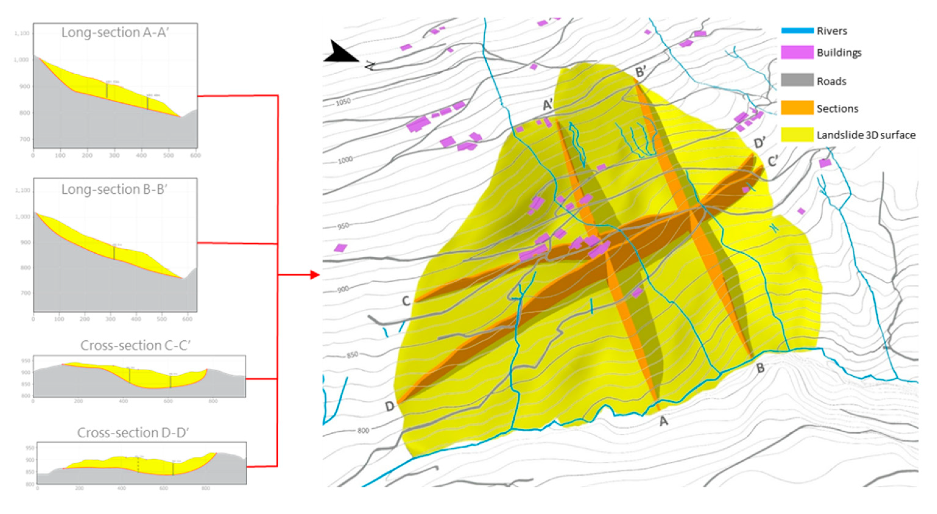
The VIM method was applied along two longitudinal (A-A’ and B-B’) and two transverse (C-C’ and D-D’) sections (Figure 1b), with the purpose of comparing the results obtained by Engl [23].

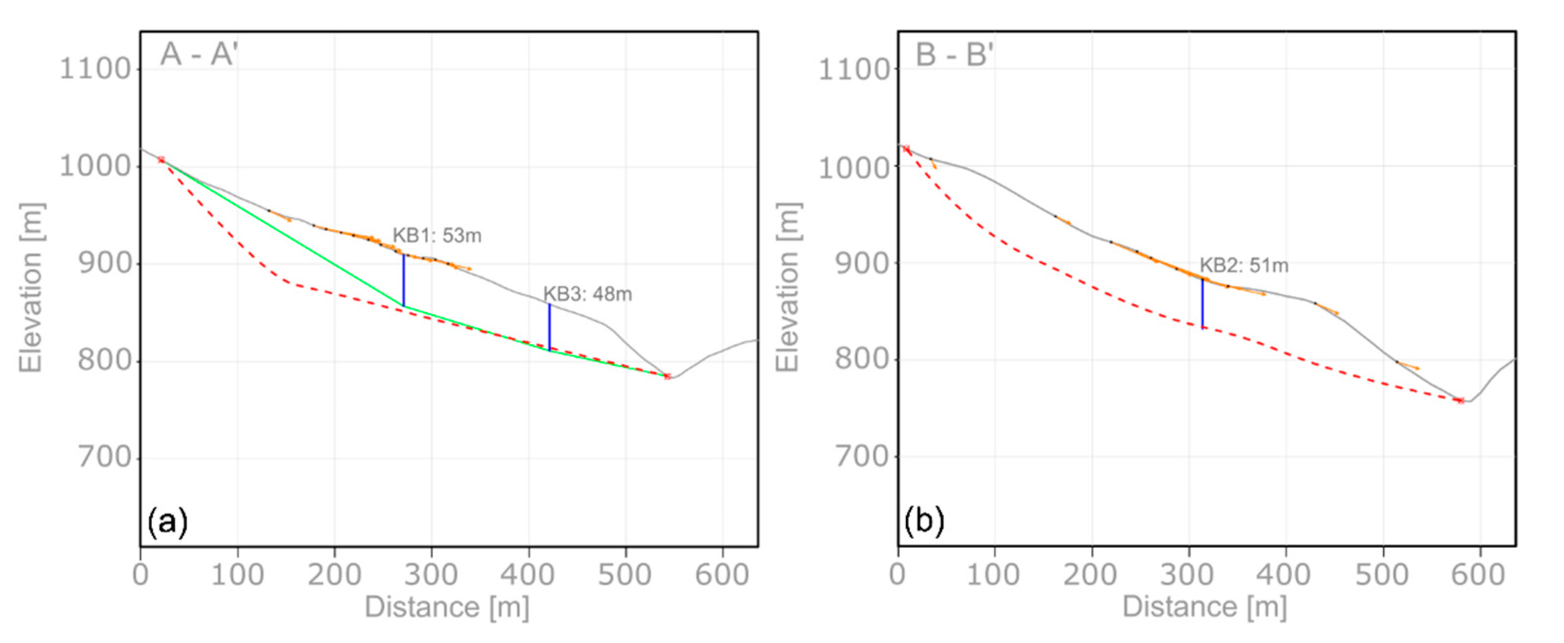
The ideal case for the application of the VIM method requires that at least one displacement vector close to the points obtained from the intersection between the profile and the landslide extent should exist. Unfortunately, for the A-A’ section (Figure 12a), the MSBAS 2D points at the toe and at the crown of the landslide were not available. The halfway point between section A-A’ and B-B’ (see Figure 1b) was the best point found in the upper part to be associated to the crown of the section A-A’, whereas the closest point to the toe is used as the last point of the long section A-A’ in the lower part.

The result was obtained only by applying the VIM method from the toe to the crown of the landslide. This profile was compared successfully with the slip-surface geometry extracted by [23] using the two boreholes (KB1 and KB3, Figure 12a) information.

For the B-B’ section, we could exploit MSBAS 2D points entirely, thanks to the wide availability of MPs both at the toe and at the crown of the landslide. The sliding surface in this section (Figure 12b) was obtained by interpolating the profiles traced in both directions (crown to toe and vice versa) and by linking the bottom part to the river bed and the upper part to the crown.

Along the C-C’ transverse section (Figure 13a), opposite immerging displacements vectors imply two types of interpretation:

• internal inhomogeneous deformation within the landslide;
• the presence of two different slabs.

In order to respect the assumptions of the VIM method, the presence of two different slabs moving rigidly was assumed.

The boundary between the two slabs corresponding to the point where the displacement immersion undergoes a complete inversion was identified. Based on this evidence, two depth profiles were independently drawn.

For slab B, the shallower sliding surface was derived by applying the geometrical approach from south to north. The final sliding surface for slab A was drawn by joining the landslide north boundary to the depth of the sliding surface obtained in A-A’ and B-B’, which intercept the plane of the section C-C’.

The geometrical construction of the sliding surface for the D-D’ cross section (Figure 13b) followed the same approach as the C-C’ cross section.

However, unlike the C-C’ section where slab A and B resulted juxtaposed, in this case, the result achieved for the shallower sliding surface of body B is more realistic. In fact, it is plausible that the blue dashed line in Figure 13b should represent the real termination of slab B that overlay slab A on the intersection zone.

The result derives from the application of the VIM in both directions (south to north and vice versa).

The final 3D landslide model (Figure 14) was generated by merging the four deep profiles in the GIS environment. More in detail, profiles A-A’ and B-B’ were taken as shown in Figure 12. On the other hand, for the transverse section, an assumption was made. Since no boreholes were available for slab B, we unified the two slabs into one. Once the three-dimensional sliding surface of the landslide was delineated using the 3D Analyst extension in ArcGIS Pro, the Cut Fill tool (Spatial Analyst toolbox) was applied in order to obtain the volume of the landslide. The volume of material mobilized calculated was estimated to be approximately 10 million of m³.

5. Discussion and Conclusions

The BFAST can detect breaks in trends and seasonality curves separately and it can be easily implemented in R open source code. For the purpose of our study, only Sentinel-1 data were used, but other sensors with similar long time series, even with lower number of observations per year (such as ENVISAT, ERS, Cosmo, TSX, ALOS), can be suited to the method. BFAST was originally born for NDVI (Normalized Difference Vegetation Index) monitoring. This latter index, derived from optical images, has a different temporal trend compared to time series derived from SAR. NDVI manifests mostly a periodic trend, whereas SAR data are not characterised by periodic acceleration and deceleration trends.

Concerning the kinematical aspect of the landslide, the best results obtained from the application of the BFAST methods were found in the slab A in terms of magnitude, change of direction, number and correspondence of BPs, and identification of the events. This result was satisfactory for the Up-Down (Figure 9) and for the East-West displacement direction. This outcome may be linked to the fact that fast velocity movements (for the slab A) can be better decomposed by the MSBAS method than the slower ones exhibited by the slab B).

Furthermore, it can be noticed that the first BP identified in slab A and at the intersection zone slightly precedes the one of slab B. This could suggest that slab A is activated before slab B.

The most representative MSBAS values matching the ATTS measurements for slab A and slab B are very close to the in-situ stations. This implies the adherence to the landslide rigid body model assumption and assumed homogeneous deformation. At the intersection zone in Figure 1b, a good representation in trend is recognised by the BFAST but the combined effect of the two distinctive deformation regimes (slab A and B) complicates the interpretation of the MSBAS results. In fact, the most representative MSBAS point found thus far from the in-situ station, indicating probably that in the intersection area the deformation is inhomogeneous.

The movement direction that has provided the best results in all three areas is the EW. This happens probably because the major displacement components of the landslide, measured at the ATTS, are along the EW direction; furthermore, the MSBAS also combined method measures for the most accurate displacement component on the horizontal plane in the EW direction.

Conversely, the MSBAS 3D gives the poorest results along the North-South direction because of acquisition geometry issues. Moreover, this technology has been recently developed and needs further improvements.

Overall, for slab A and for the intersection zone, the BFAST approach produces the best results since the algorithm is able to find four break points for each MSBAS time series, as well as for the two ATTS (with the only exception of point n. P6432 in Figure 10 with only three BPs found). On the other hand, for slab B, the loss of BPs in the ATTS as well as in the MSBAS can be related to the fact that the original displacement time series are linear in comparison to the previously mentioned cases. We can probably suppose that BFAST is not able to associate a BP to a subtle and very gentle change in the time series slope.

The advantages of BFAST is that we can study the activation for all three distinctive slabs, and in three different directions obtain very close results to the in-situ measurements in terms of trend reconstruction and break segmentation. Other authors [20] used only the fastest station located in slab A or the average of 14 stations [23] by interpolating only the horizontal directions and discarding the evolution of the vertical deformation in time. Those two latter approaches were useful to identify hydro-meteorological triggering events (summarised in Table 1) but cannot be effective to study compound two-slab landslide, which implies a roto-translational motion as with the Vögelsberg case.

Further remarks concerning the application of the MSBAS 3D is that in the case of slab B, where the velocity of deformation is already below the precision of MT-InSAR velocity threshold [36], the extraction of the NS components lead to the underestimation of the newly derived UD and EW direction of displacement compared with the results derived by MSBAS 2D.

The main advantage of the VIM method is that its application allows the reconstruction of the depth of the landslide sliding surface mostly using SAR data. The method is easy and quick to apply but the best results are obtained when the method is applied along the slope direction (for longitudinal profiles).

The limit of this method, however, is that when no points are present at the toe or at the crown of the landslide; therefore, in-situ data are needed. This is a very important aspect, especially for longitudinal sections.

Concerning the transverse sections, the results obtained show that the method is able to identify both slabs (A and B). However, the Vögelsberg landslide is a very complex case study, since in the intersection area, which does not move as a rigid body, the VIM hypothesis are no longer valid; some uncertainties for the cross sections on delineating the slab B surface were solved by considering a unique landslide body for the 3D reconstruction.

A better 3D landslide reconstruction is expected by applying the proposed workflow to other case studies consisting of single landslide body, or by exploiting other sources of data, such as Ground based-SAR, looking at the landslide with the North-South line of sight and paired to MSBAS 2D (East-West and Up-Down) data.

Overall, this paper highlighted that the identification of trends in landslide kinematics and the estimation of the sliding surface depth by exploiting DInSAR data are feasible tasks. These outcomes can be adopted for landslide hazard assessment within the definition of strategies for landslide risk analysis.

References

1. Crosta, G.B.; Frattini, P.; Agliardi, F. Deep seated gravitational slope deformations in the European Alps. Tectonophysics 2013, 605, 13–33. [Google Scholar] [CrossRef]
2. Cruden, D.M.; Varnes, D.J. Landslides: Investigation and Mitigation. Chapter 3-Landslide Types and Processes; Transportation Research Board Special Report; National Academy Press: Washington, DC, USA, 1996. [Google Scholar]
3. Zangerl, C.; Eberhardt, E.; Perzlmaier, S. Kinematic behaviour and velocity characteristics of a complex deep-seated crystalline rockslide system in relation to its interaction with a dam reservoir. Eng. Geol. 2010, 112, 53–67. [Google Scholar] [CrossRef]
4. Crosta, G.B.; Di Prisco, C.; Frattini, P.; Frigerio, G.; Castellanza, R.; Agliardi, F. Chasing a complete understanding of the triggering mechanisms of a large rapidly evolving rockslide. Landslides 2014, 11, 747–764. [Google Scholar] [CrossRef]
5. Zangerl, C.; Holzmann, M.; Perzlmaier, S.; Engl, D.; Strauhal, T.; Prager, C.; Steinacher, R.; Molterer, S. Characterisation and Kinematics of Deep-Seated Rockslides in Foliated Metamorphic Rock Masses; Springer: Berlin/Heidelberg, Germany, 2015; pp. 571–575. [Google Scholar]
6. Hungr, O.; Leroueil, S.; Picarelli, L. The Varnes classification of landslide types, an update. Landslides 2014, 11, 167–194. [Google Scholar] [CrossRef]
7. Eberhardt, E.; Stead, D.; Coggan, J.S. Numerical analysis of initiation and progressive failure in natural rock slopes—The 1991 Randa rockslide. Int. J. Rock Mech. Min. Sci. 2004, 41, 69–87. [Google Scholar] [CrossRef]
8. Agliardi, F.; Crosta, G.B.; Frattini, P. Slow rock-slope deformation. Landslides Types Mech. Modeling 2012, 23, 207. [Google Scholar]
9. Stead, D.; Eberhardt, E. Understanding the mechanics of large landslides. Ital. J. Eng. Geol. Environ. Book Ser. 2013, 6, 85–112. [Google Scholar]
10. Riva, F.; Agliardi, F.; Amitrano, D.; Crosta, G.B. Damage-based time-dependent modeling of paraglacial to postglacial progressive failure of large rock slopes. J. Geophys. Res. Earth Surf. 2018, 123, 124–141. [Google Scholar] [CrossRef] [Green Version]
11. Hutchinson, J.N. General report: Morphological and geotechnical parameters of landslides in relation to geology and hydrogeology. In Proceedings of the 5th International Symposium on Landslides, Lausanne, Switzerland, 10–15 July 1988; Bonnard, C., Ed.; pp. 3–35. [Google Scholar]
12. Cody, E.; Draebing, D.; McColl, S.; Cook, S.; Brideau, M.A. Geomorphology and geological controls of an active paraglacial rockslide in the New Zealand Southern Alps. Landslides 2019, 17, 775–776. [Google Scholar] [CrossRef]
13. Vick, M.; Böhme, M.; Rouyet, L.; Bergh, S.G.; Corner, G.D.; Lauknes, T.R. Structurally controlled rock slope deformation in northern Norway. Landslides 2020, 17, 1745–1776. [Google Scholar] [CrossRef]
14. Strauhal, T.; Zangerl, C.; Fellin, W.; Holzmann, M.; Engl, D.; Brandner, R.; Tropper, P.; Tessadri, R. Structure, mineralogy and geomechanical properties of shear zones of deep-seated rockslides in metamorphic rocks (Tyrol, Austria). Rock Mech. Rock. Eng. 2017, 50, 419–438. [Google Scholar] [CrossRef]
15. Zangerl, C.; Fey, C.; Prager, C. Deformation characteristics and multi-slab formation of a deep-seated rock slide in a high alpine environment (Bliggspitze, Austria). Bull. Eng. Geol. Environ. 2019, 78, 6111–6130. [Google Scholar] [CrossRef] [Green Version]
16. Samsonov, S.; d’Oreye, N. Multidimensional time series analysis of ground deformation from multiple InSAR data sets applied to Virunga Volcanic Province. Geophys. J. Int. 2012, 191, 1095–1108. [Google Scholar]
17. Samsonov, S.; d’Oreye, N. Multidimensional Small Baseline Subset (MSBAS) for Two-Dimensional Deformation Analysis: Case Study Mexico City. Can. J. Remote Sens. 2017, 43, 318–329. [Google Scholar] [CrossRef]
18. Samsonov, S.; Dille, A.; Dewitte, O.; Kervyn, F.; d’Oreyede, N. Satellite interferometry for mapping surface deformation time series in one, two and three dimensions: A new method illustrated on a slow-moving landslide. Eng. Geol. 2020, 266, 105471. [Google Scholar] [CrossRef]
19. Intrieri, E.; Frodella, W.; Raspini, F.; Bardi, F.; Tofani, V. Using Satellite Interferometry to Infer Landslide Sliding Surface Depth and Geometry. Remote Sens. 2020, 12, 1462. [Google Scholar] [CrossRef]
20. Pfeiffer, J.; Zieher, T.; Schmieder, J.; Rutzinger, M.; Strasser, U. Spatio-temporal assessment of the Hydrological drivers of an active deep-seated gravitational slope deformation: The Voegelsberg landlslide in Tyrol (Austria). Earth Surf. Process. Landf. 2021, 46, 1865–1881. [Google Scholar] [CrossRef]
21. Verbesselt, J.; Hyndman, R.; Newnham, G.; Culvenor, D. Phenological change detection while accounting for abrupt and gradual trends in satellite image time series. Remote Sens. Environ. 2010, 114, 2970–2980. [Google Scholar] [CrossRef] [Green Version]
22. Rockenschaub, M.; Kolenprat, B.; Nowotny, A. Innsbrucker quarzphyllitkomplex, tarntaler mesozoikum, patscherkofelkristallin. Geologische Bundesanstalt—Arbeitstagung 2003, Blatt 148 Brenner, pp. 41–58. unpublished report.
23. Engl, D. Aktueller Kenntnisstand Hangbewegung Vögelsberg, Gemeinde Wattens Forsttechnischer Dienst für Wildbach- und Lawinenverbauung. Innsbruck. 2018. Not published geological report from the Torrent and Avalanches Control (WLV).
24. Ludwig, T.; Außerlechner, R. Hangbewegungen und deren Auswirkungen auf Wohn- und Wirtschaftsgebäude im Alpenraum am Beispiel Vögelsberg. 23. Geoforum Umhausen Tirol, 14–15 October 2021. Online Resource. Available online: https://atnastablobgeoforumarc01.blob.core.windows.net/geoforumarchive001/Tagungsband%2023%20Geoforum%20Umhausen%202021.pdf (accessed on 18 May 2022).
25. Derauw, D.; d’Oreye, N.; Jaspard, M.; Caselli, A.; Samsonov, S. Ongoing automated ground deformation monitoring of Domuyo —Laguna del Maule area (Argentina) using Sentinel-1 MSBAS time series: Methodology description and first observations for the period 2015–2020. J. South Am. Earth Sci. 2020, 104, 102850. [Google Scholar] [CrossRef]
26. Verbesselt, J.; Hyndman, R.; Newnham, G.; Culvenor, D. Detecting trend and seasonal changes in satellite image time series. Remote Sens. Environ. 2010, 114, 106–111. [Google Scholar] [CrossRef]
27. Masiliunas, D.; Tsendbazar, N.-E.; Herold, M.; Verbesselt, J. BFAST Lite: A Lightweight Break Detection Method for Time Series Analysis. Remote Sens. 2021, 13, 3308. [Google Scholar] [CrossRef]
28. Saatchi, S.; Asefi-Najafabady, S.; Malhi, Y.; Aragão, L.E.O.C.; Anderson, L.O.; Myneni, R.B.; Nemani, R. Persistent effects of a severe drought on Amazonian forest canopy. Proc. Natl. Acad. Sci. USA 2012, 110, 565–570. [Google Scholar] [CrossRef] [PubMed] [Green Version]
29. Watts, L.M.; Laffan, S.W. Effectiveness of the BFAST algorithm for detecting vegetation response patterns in a semi-arid region. Remote Sens. Environ. 2014, 154, 234–245. [Google Scholar] [CrossRef]
30. Hamunyela, E.; Verbesselt, J.; Herold, M. Using spatial context to improve early detection of deforestation from Landsat time series. Remote Sens. Environ. 2016, 172, 126–138. [Google Scholar] [CrossRef]
31. Tsutsumida, N.; Saizen, I.; Matsuoka, M.; Ishii, R. Land Cover Change Detection in Ulaanbaatar Using the Breaks for Additive Seasonal and Trend Method. Land 2013, 2, 534–549. [Google Scholar] [CrossRef]
32. Yang, Y.; Wang, Y. Using the BFAST Algorithm and Multitemporal AIRS Data to Investigate Variation of Atmospheric Methane Concentration over Zoige Wetland of China. Remote Sens. 2020, 12, 3199. [Google Scholar] [CrossRef]
33. Zhu, M.; Wan, X.; Fei, B.; Qiao, Z.; Ge, C.; Minati, F.; Vecchioli, F.; Li, J.; Costantini, M. Detection of Building and Infrastructure Instabilities by Automatic Spatiotemporal Analysis of Satellite SAR Interferometry Measurements. Remote Sens. 2018, 10, 1816. [Google Scholar] [CrossRef] [Green Version]
34. Carter, M.; Bentley, S.P. The geometry of slip surfaces beneath landslides: Predictions from surface measurements. Can. Geotech. J. 1985, 22, 234–238. [Google Scholar] [CrossRef]
35. Cruden, D.M. The geometry of slip surfaces beneath landslides: Predictions from surface measurements: Discussion. Can. Geotech. J. 1986, 23, 94. [Google Scholar] [CrossRef]
36. Cascini, L.; Peduto, D.; Pisciotta, G.; Arena, L.; Ferlisi, S.; Fornaro, G. The combination of DInSAR and facility damage data for the updating of slow-moving landslide inventory maps at medium scale. Nat. Hazards Earth Syst. Sci. 2013, 13, 1527–1549. [Google Scholar] [CrossRef]
Figure 1. (a) location of the Vögelsberg DSGSD (in purple), the analyzed slow-moving rockslide (in red), and the shallow debris slide (in blue), underground Open Street Map overlaid to digital elevation model (1.3 × vertical exaggeration); (b) location of the in-situ and ancillary data available for the Vögelsberg rock slide together with the longitudinal (A-A’ and B-B’) and cross profiles (C-C’ and D-D’) selected for the application of the VIM method using MSBAS.
Geosciences 12 00256 g001
Figure 2. MSBAS 2D and 3D workflow adopted to process the ascending and descending data image stacks acquired by Sentinel-1 radar sensor.
Geosciences 12 00256 g002
Figure 3. MSBAS velocities (a) and ATTS time series (b) for the East–West (EW) direction of motion at the Vögelsberg landslide.
Geosciences 12 00256 g003
Figure 4. MSBAS velocities (a) and ATTS time series (b) for the North-South (NS) direction of motion at the Vögelsberg landslide.
Geosciences 12 00256 g004
Figure 5. MSBAS velocities (a) and ATTS time series (b) for the Up-Down (UD) direction of motion at the Vögelsberg landslide.
Geosciences 12 00256 g005
Figure 6. The workflow of the adopted methodology.
Geosciences 12 00256 g006
Figure 7. BFAST applied to the vertical component of the MSBAS point n. 7021 showing the original time series (Yt), decomposed in seasonal (St), trend (Tt), and error (et) component.
Geosciences 12 00256 g007
Figure 8. Schematic representation of VIM method.
Geosciences 12 00256 g008
Figure 9. Vertical displacement time series correlation of ATTS (red) against MSBAS (green) for slab A. Evaluation of Trends and BPs of point n. P7021 plotted against total cumulative precipitation (dark blue line), cumulative 7-days precipitation (histogram), and snow depth (light blue line).
Geosciences 12 00256 g009
Figure 10. Horizontal (EW) displacement time series correlation of ATTS (red) against MSBAS (purple) for the intersection zone. Evaluation of Trends and BPs of point n. P6432 plotted against total cumulative precipitation (dark blue line), cumulative 7-days precipitation (histogram), and snow depth (light blue line).
Geosciences 12 00256 g010
Figure 11. Horizontal (EW) displacement time series correlation of ATTS (red) against MSBAS (gold) for slab B. Evaluation of Trends and BPs of point n. P7472 plotted against total cumulative precipitation (dark blue line), cumulative 7-days precipitation (histogram), and snow depth (light blue line).
Geosciences 12 00256 g011
Figure 12. VIM results for the A-A’ (a) and B-B’ (b) cross sections, landslide surface (red dotted line), landslide surface produced by [23] (green dotted line), boreholes position (blue lines), and MSBAS data (orange vectors).
Geosciences 12 00256 g012
Figure 13. VIM results for the C-C’ (a) and D-D’ (b) transverse sections, with landslide boundaries (red dots), depth from sections A-A’ and B-B’ (green dots), intersection zone (purple dots), and MSBAS data (orange vectors).
Geosciences 12 00256 g013
Figure 14. 3D landslide model reconstruction built by merging the previously VIM-derived sections.
Geosciences 12 00256 g014