Abstract
Known as the “lung of the planet”, the Amazon rainforest produces more than 20% of the Earth’s oxygen. Once a carbon pool for mitigating climate change, the Brazilian Amazônia Biome recently has become a significant carbon emitter due to increasingly frequent wildfires. Therefore, it is of crucial importance for authorities to understand wildfire dynamics to manage them safely and effectively. This study incorporated remote sensing and spatial statistics to study both the spatial distribution of wildfires during 2019 and their relationships to 15 environmental and anthropogenic factors. First, broad-scale spatial patterns of wildfire occurrence were explored using kernel density estimation, Moran’s I, Getis-Ord Gi*, and optimized hot spot analysis (OHSA). Second, the relationships between wildfire occurrence and the environmental and anthropogenic factors were explored using several regression models, including Ordinary Least Squares (OLS), global (quasi) Poisson, Geographically-weighted Gaussian Regression (GWGR), and Geographically-weighted Poisson Regression (GWPR). The spatial analysis results indicate that wildfires exhibited pronounced regional differences in spatial patterns in the vast and heterogeneous territory of the Amazônia Biome. The GWPR model outperformed the other regression models and explained the distribution and frequency of wildfires in the Amazônia Biome as a function of topographic, meteorologic, and environmental variables. Environmental factors like elevation, slope, relative humidity, and temperature were significant factors in explaining fire frequency in localized hotspots, while factors related to deforestation (forest loss, forest fragmentation measures, agriculture) explained wildfire activity over much of the region. Therefore, this study could improve a comprehensive study on, and understanding of, wildfire patterns and spatial variation in the target areas to support agencies as they prepare and plan for wildfire and land management activities in the Amazônia Biome.
1. Introduction
Fire occupies a unique position in environmental history. It can have both beneficial and harmful effects on the environment. The Amazon rainforest is the world’s largest tropical rainforest, with an area of more than 5 million square kilometers [1]. It serves as one of Earth’s largest reservoirs of carbon dioxide, which plays a critical role in global and regional carbon and water cycles, and it provides important ecological services to our planet [2]. However, it is observed that year 2019 was the worst fire to hit the Amazon Rainforest for over a decade [3]. There were more than 80,000 fires in 2019 in Amazon, which was a nearly 80 percent jump compared to that in 2018, according to Brazil’s National Institute for Space Research [4]. The growing problem of wildfires threatens the ecological balance of nature in the Amazon rainforest and affects forest biodiversity. Meanwhile, combusted vegetation emits large quantities of trace gases (e.g., , , and ), particulates, and smoke into the atmosphere, which causes air pollution. Moreover, forest structure and species composition probably require more than decades or centuries to recover. To sum up, wildfires can cause severe, long-term environmental, socioeconomic, and public health impacts worldwide. The Amazon may not belong to all of us, but what happens there affects all of us. Therefore, understanding and projecting the spatial patterns of wildfire and its significant driving factors are critical for government and relevant departments to prepare for changes in environmental threats, develop wildfire supervision and risk reduction strategies, and make sustainable fire management decisions.
The spatial distribution of wildfire is influenced by various factors and has certain regularity, and it often displays a continuous periodic law in time and aggregation law in space [5]. Wittenberg and Malkinson [6] analyzed the spatial distribution characteristics of wildfires in mixed pine forests in the Mediterranean region by analyzing spatial data and establishing logistic regression models. They pointed out that the spatial distribution of wildfires in Carmel Mountain in Israel was not random, and the locations of the observed fires in this area were closer to the roadside. Liu et al. [7] studied the spatio-temporal distribution of wildfires in Sichuan province, China, from 2001 to 2012. They found that peak periods of wildfires were from January to May, and the number of forest fires continued to rise every year. In terms of spatial pattern, forest fires were clustered at smaller spatial scales.
Meanwhile, exploring wildfire drivers is crucial to developing wildfire prediction models. Genton et al. [8] used point pattern analysis to study the spatial pattern of wildfire occurrences in north-eastern Florida. The results revealed that occurrences of lightning, arson, and railroad are spatially more clustered than occurrences of other accidental causes. Román-Cuesta and Martínez-Vilalta [9] used spatial buffer zone and Spearman’s correlations to investigate relationships between road density, agricultural land expansion, and wildfire within Biosphere Reserves in Mexico.
In order to reduce wildfire risk, and minimize damages to the ecosystem and human beings, statistical modeling has played a crucial role in the quantitative analysis of wildfire occurrences and their driving factors. With the deepening of research, many scholars recognize that spatial heterogeneity is necessary to be considered. Using a single equation with a set of parameters for describing the entire study area often has limitations in explaining a nonlinear relationship. Therefore, Fotheringham et al. [10] proposed geographically weighted regression (GWR) as a method of modeling spatially non-stationary fires across locations. Koutsias et al. [11] applied the OLS (Ordinary Least Squares) regression model, GWR model, classical logistic regression model, and GWR logistic model to analyze the occurrence of wildfire in southern Europe. Their results indicate that GWR models were more appropriate than the classical global ones. Avila-Flores et al. [12] used the GWR method to determine contributing factors that are spatially associated with wildfire occurrence in the State of Durango, Mexico. Their results showed that land-use change is one of the main explanatory variables for the spatial pattern of wildfires throughout the study area. Furthermore, vegetation type and precipitation play important roles, as well.
Though contributing factors and spatial distributions of wildfires have been considered in relevant studies in many regions over the world, it has been challenging to identify a set of key wildfire drivers under a specific environment, and an interaction between bottom-up and top-down forces is often complex and unpredictable [13]. Such knowledge is not yet sufficiently developed for application in the real world. For instance, Brazil’s National System for Forest Fire Prevention and Control has tried to allocate fire control resources by evaluating the municipalities that experienced the most fires in previous years, but the result is not satisfied with only a 30% accuracy rate [14]. In summary, the relationship between wildfire and its drivers varies not only by scale but also by region. So, all of these make the site-specific case studies necessary.
This study attempts to establish large-scale wildfire occurrence models in the Amazônia Biome. To overcome the constraints of traditional regression modeling which assumes stationary processes [10], Geographically Weighted Gaussian Regression (GWGR) and Geographically Weighted Poisson Regression (GWPR) models are applied for the first time for wildfire studies in Amazônia Biomes. In addition to topographic and meteorologic factors, this study considers several habitat configuration metrics, aiming finding relationships between forest fragmentation and wildfire. These issues have rarely been systematically studied in the Amazônia Biome. Therefore, we compared two different wildfire prediction models in spatial statistic methods and analyze the spatial pattern of wildfire distribution in the Amazon Biome. The two specific objectives include (1) revealing the spatial variation of broad-scale wildfire occurrence patterns in the Amazônia Biome in 2019 using spatial analysis approaches; (2) assessing performances of the modeling approaches which is more suitable for characterizing wildfire spatial patterns and addressing driving factors. This research aims at improving a comprehensive study on, and understanding, of fire regime and risk factors. The results are expected to offer valuable insights into land and fire management practices and predictions. The developed modeling framework could be tailored to investigate the spatial pattern of wildfire occurrence in other rainforest regions facing similar issues. The knowledge gained from Amazônia Biome could also be used to inform other vulnerable rainforest regions globally to reduce threats and potential damages from wildfires.
2. Study Area
The area chosen for this study (Figure 1) is the Brazilian Amazônia Biome, which covers nine states and an area of 4.2 million km2 mostly composed of evergreen forests, but also including grasslands, wetlands, and areas converted by farming and cattle ranching. The climate is characterized by warm temperature (ranging from 24 to 27 °C across a year), high rainfall (around 3200 mm/year), and high relative humidity (from 80% to 94%, across a year) [15].
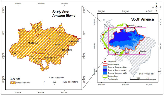
Figure 1.
Location of the study area.
3. Data Sets and Methodology
3.1. The Workflow of the Study
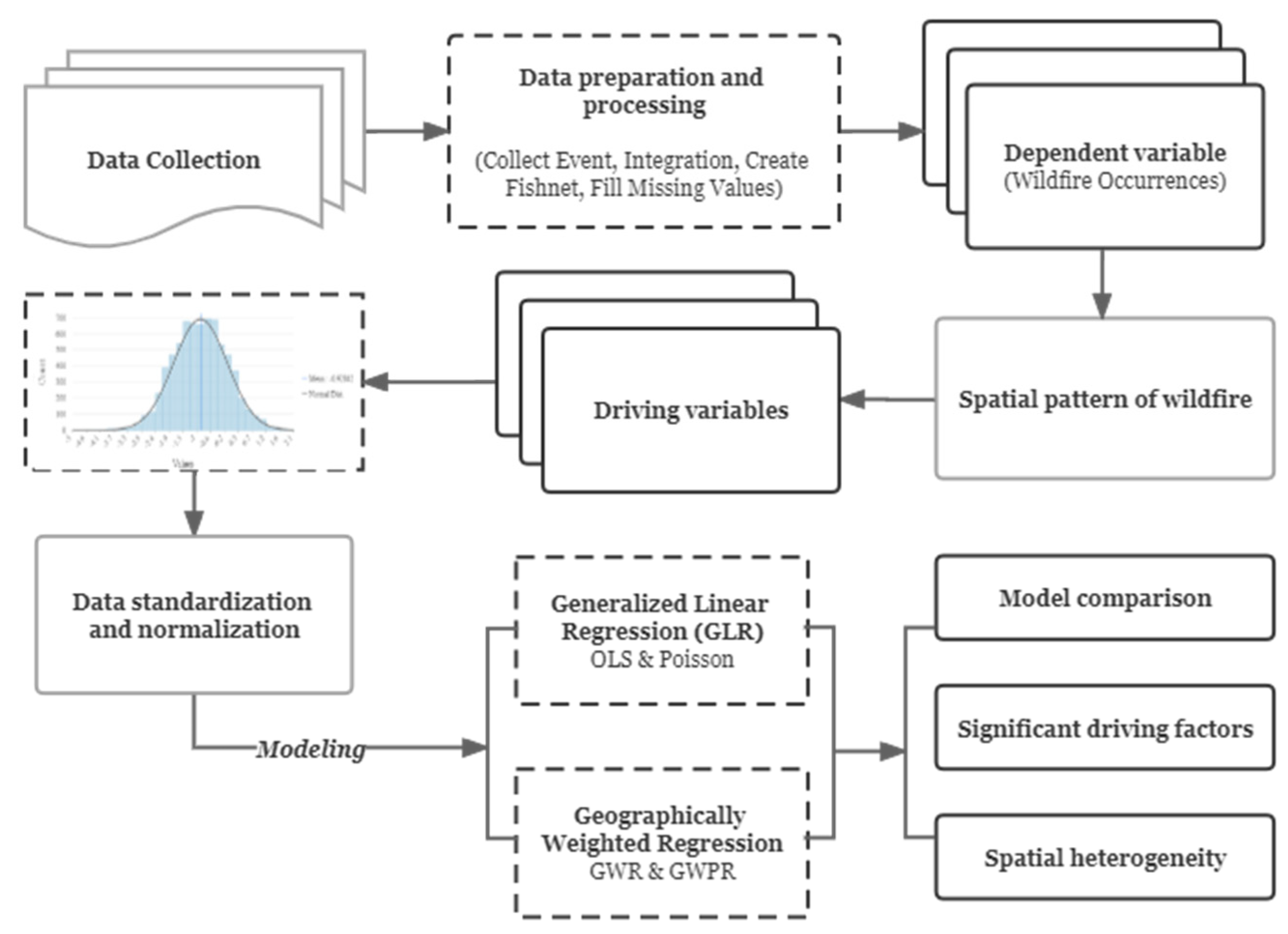
Figure 2 shows the overall workflow of this study. The first step was to prepare and process the wildfire data. We moderated the inaccurate GPS coordinate positioning and transformed wildfire incidents into weighted points data. Second, spatial analysis methods of kernel density, spatial autocorrelation (Global Moran’s I), and hot spot analysis were adopted to reveal spatial patterns of wildfire. Then, the wildfire data and 15 explanatory variables data were sampled for model building. During the model building process, the skewed dependent variable and explanatory variables are unsuitable for conducting regression analysis and can reduce the model accuracy when building linear regression models, e.g., OLS and classic GWR models. Therefore, we adopted the logarithm transformation for the dependent variable and the unconditional Box-Cox transformation for the explanatory variables. Then, all explanatory variables were standardized for eliminating the dimensions and balancing the contribution of each factor. We calculated the Variance Inflation Factor (VIF) value by OLS to assess and eliminate multicollinearity.
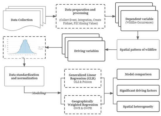
Figure 2.
The logical framework of the study.
3.2. Data Preparation and Processing
3.2.1. Wildfire Data (Dependent Variable)
In this study, wildfire occurrences are the dependent variable. The wildfire data were accessed from the MODIS’s MCD14ML global monthly fire location product provided by LANCE FIRMS operated by NASA ESDIS (https://firms.modaps.eosdis.nasa.gov, accessed on 16 April 2021), which provides monthly geospatial information, including location, date, confidence, and additional information for each 1 km fire pixel detected by Terra and Aqua MODIS sensors. As a result of the high sensitivity and quantization accuracy provided by the MODIS sensor and two times a day temporal resolution, this product has been widely utilized in wildfire studies. We chose the MCD14ML because it has been demonstrated as a reliable source to monitor and analyze wildfires at local, regional, and global scales [16,17]. In many previous studies, the exact location of the wildfire ignition points (x, y coordinates) was used as a dependent variable in statistical models [6,8,11], but the accuracy of the spatial location of wildfires significantly varies depending on the data source. The MCD14ML resolution is 1 km, and the fire point is interpreted as one or more fires that have been detected within 1 km of each fire source location. Therefore, the interpretation results may deviate from the actual ignition location. To alleviate the deviation, we used a grid pattern analysis in this study to provide a comprehensive and uniform method to reflect the spatial properties of variables. Given the fact that the area of Amazônia Biome is about 4.2 million km2, we created a fishnet-like grid to set the study areas into 20 km × 20 km (a total of 7158 grids) and calculated the total number of wildfire points in each grid. In addition, we filled in missing values for several layers to conduct an effective spatial analysis of the entire study area. The frequency of wildfire occurrences is a positive skew, which means pixels with zero fire counts are much higher frequency.
3.2.2. Driving Factors (Explanatory Variables)
Based on an extensive literature review [18,19] and available data, the explanatory variables in this study include four broad categories: (1) topographic, (2) vegetation cover and land use, (3) anthropogenic, and (4) meteorological, with a total of 15 explanatory variables (Table 1). The topographic variables include elevation, slope, and aspect. Previous work suggested that wildfires are prone to burn on flat, ridges, and steep north-facing slopes, while valleys and steep south-facing slopes are the least likely to burn [20]. Aspect is a circular variable that cannot be used in linear statistics, so the layer was cosine-transformed to obtain a linear index that can better distinguish the degree of exposure [21]:
where θ is the degree of aspect and the range is 0–360°. The values of the aspect index ranged from −1 (southward) to 1 (northward).

Table 1.
Sources and descriptions for variables.
Variables in vegetation cover and land use include: (1) Fractional Vegetation Cover (FVC), (2) Number of Forest Patches (NFP), (3) Edges Proportion (EP), (4) Pastureland Areas, and (5) Cropland Areas). FVC is calculated based on the NDVI, it is used to represent the corresponding fuel amount within the grid. In addition, based on previous research, the interaction between deforestation, forest fragmentation, and wildfires is clear in the Amazon rainforest [22,23]. Pieces of large, contiguous, forested areas are deforested and separated for purpose of human development [24], which activities directly caused forest fragmentation, resulting in increased light intensity, higher daytime temperature, higher wind speed, and lower humidity. Wildfire has a higher tendency to spread in fragmented landscapes with smaller patches of forest and more edges. Therefore, the NFP and EP were used in this study. NEP calculated the number of forest patches within a cell. EP is the sum of the lengths of all forest edge segments within a cell, divided by cell area. Wildfires in the Amazon are largely caused by the extensive conversion of forests and agricultural practices [16]. The land use variables in pastureland area and cropland area were also considered in this study. It is the sum of (Pasture/Crop-) areas within a cell, divided by the total cell area, and multiplied by 100.
Many previous studies indicate that the majority of wildfires are anthropogenic or accident-caused, indicating a connection between human-caused factors and wildfire occurrence [25,26]. In this study, the anthropogenic factors included socioeconomic variables (population density), infrastructural variables (road density), and forest loss (percentage of deforestation).
The weather or climate factors are top-down controls on wildfires that have been emphasized in several regional and continental studies [27,28,29,30,31,32]. In this study, ambient weather elements include average annual temperature (°C), relative humidity, wind speed (m/s), and maximum cumulative water deficit (MCWD) (mm). Temperature determines the combustibility of fuels. Humidity and precipitation affect the moisture level of fuel [33]. Wind speed is also one of the most important factors because it can produce a fresh supply of oxygen as well as push the wildfire toward a new source of fuel [34]. Water stress in tropical forests is often measured by the MCWD. This metric was proposed by Aragão et al. [35], and, in different parts of the Amazon Rainforest, the amount of evapotranspiration (E) is usually about 100 mm per month on average. Thus, monthly precipitation below 100 mm means that more water will be lost and evaporation will be greater than precipitation, thus generating a water deficit state. We performed Map algebra operations on the basis of the global annual precipitation data to obtain the average monthly precipitation data and subtract 100 mm from monthly precipitation values. Then, the most negative (minimum) monthly MCWD value for each pixel was used. Figure 3a illustrates the spatial distribution of wildfire points and Figure 3b–p presents the spatial distribution of explanatory variables.
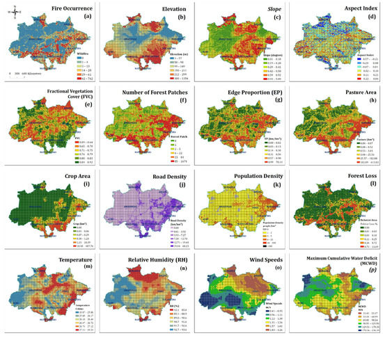
Figure 3.
Spatial distribution of dependent and explanatory variables. (a) Wildfire count, (b) Elevation, (c) Slope, (d) Aspect, (e) FVC, (f) Number of Forest Patches, (g) Edge Proportion, (h) Pasture Area, (i) Crop Area, (j) Road Density, (k) Population Density, (l) Forest Loss, (m) Temperature, (n) Relative Humidity, (o) Wind Speed, (p) Maximum Cumulative Water Deficit.
3.3. Spatial Pattern Analyses
3.3.1. Spatial Density
Kernel Density Estimation (KDE) is one of the useful tools for determining the spatial intensity of a point process, and understanding and predicting potentially event patterns [36]. It describes the global trend of a parameter, and the KDE method uses kernel density interpolation to reveal the distribution of event points in the study area [37]. The created continuous surface can minimize the effect of fire location uncertainty [38]. The expression of the density f(x) at point x where the wildfire occurs is:
where, is the kernel function; > 0 is a smoothing parameter called the bandwidth. x is the dataset of wildfire incidents (, , … ); X − is the distance between the estimated point to the sample point i. We applied KDE to map the distribution of wildfires in the Amazônia Biome. The implementation of this function is based on Quadratic Kernel developed by Silverman [37]. The bandwidth calculated was 9512.5 m and it was used for the kernel density estimation.
3.3.2. Hotspot Analysis
First, we used the Moran’s I index to investigate whether a spatial pattern is clustered, dispersed, or random [39]. Then, we used the hot spot analysis of wildfire events to determine where statistically significant clustering occurred. Statistical cluster analysis can help minimize the subjectivity in maps. The most commonly used tools are Getis-Ord Gi* and Optimized Hot Spot Analysis (OHSA). Getis-Ord Gi* computes a z-statistic by comparing the proximity-weighted sum of total fires at a particular parish to the sum across the entire sample to identify areas of more intense clustering of high (low) wildfire occurrence. OHSA is a new tool, which is a combination of the Incremental Spatial Autocorrelation tool and the Getis-Ord Gi*. It can calculate threshold distances directly, to create a map of statistically significant hot and cold spots.
3.4. Spatial Statistical Analyses
3.4.1. Geographically Weighted Gaussian Regression (GWGR)
In practice, with the change of geographical location, a relationship among variables will change, that is, “Spatial Nonstationarity”. Fotheringham et al. [10] compared classic GWR to a “spatial microscope” because of its ability to measure and visualize variations in relationships that are unobservable in spatial and global models. This modeling approach focuses on spatial differences and a search for exceptions or local “hot spots”. GWGR constructs a separate Ordinary Least Squares (OLS) equation for every location in the dataset, which includes the dependent and explanatory variables of locations falling within the bandwidth of each target location. Fotheringham et al. [10] gave a general form of a basic GWGR model as:
where, is the dependent variable at location i; is the explanatory variable at location i; m is the number of explanatory variables; is the intercept parameter at location i; is the local regression coefficient for the explanatory variable at location i, and is the random error at location i.
In a GWGR model, the estimation of parameters is related to the bandwidth used by the kernel function. In this study, the corrected Akaike Information Criteria (AICc) was used to select the optimum bandwidth.
3.4.2. Geographically Weighted Poisson Regression (GWPR)
Although the GWGR model can effectively resolve the spatial non-stationarity problem, this technique is only used when the distribution of the data is Gaussian. The problem of overdispersion in spatial count data is one of the most common problems encountered in reality [40], and most explanatory variables have skewness, which makes classic GWGR inappropriate to model. Since the 1970s, the Poisson regression has been regarded as a reliable method for modeling count data [41]. Therefore, in addition to transforming discrete count data to a continuous scale as described above, we can use the Poisson regression model and extend it to the classic GWGR model by adding geographical location, then the Geographically Weighted Poisson Regression (GWPR) was developed. The GWPR model is written as [42]:
where and are the GWPR model parameters that describe the location i in terms of x and y coordinates. Thus, the expected value of can be predicted by the inverse link function = . For modeling wildfire occurrence, we added a constant to the average observed number of wildfire occurrences to mitigate problems related to counts of zero.
The GWPR has been considered a reliable model for predicting wildfire occurrence, however, the model often faces the challenge of strict requirement of Poisson distribution, i.e., the mean is equal to the variance (equidispersion) or is expressed μ = E(Y) = Var(Y), where µ is the mean of the count data Y. In most cases, the observed variance is larger than the assumed variance, which is called overdispersion [43]. The number of wildfires also has the problem of overdispersion, because the zero counts tend to occur more often than higher numbers of wildfire events. If overdispersion is ignored, the model fitting will underestimate the standard errors for Poisson regression model coefficients and lead to biased hypothesis testing. The quasi-Poisson model is an effective way to adjust for dispersion, which introduces a dispersion parameter into the Poisson variance so that the Poisson model is scaled [44]. The dispersion parameter () is estimated by deviance or Pearson’s χ2 test statistic divided by its degrees of freedom from the Goodness-of-Fit test. If the estimated dispersion is >1, the data may be over-dispersed, while a dispersion <1 indicates that the data may be under-dispersed. The quasi-likelihood requires the standard errors generated from the Poisson model to be multiplied by the factor , which is the square root of the dispersion parameter:
This scaled the “quasi-Poisson” regression model, which has the same mean function as the Poisson regression model but with a variance that is times the mean as represented by [44]:
The model is fit in a usual way, and the resulting parameter coefficients would be the same as the estimated regression coefficients from the Poisson model, but only the standard errors of the coefficients would be larger. The t statistic is the coefficient divided by its standard error. Once we find this t-test statistic, we typically find the p-value associated with it.
The best bandwidth size was determined automatically using the golden section search method, based on the lowest AICc. The kernel type and function for geographic weighting to estimate local coefficients for each fishnet grid and bandwidth size was a Gaussian kernel with adaptive bandwidth, which was appropriate because the regression points were irregularly positioned in the study area. The deviance/df ratio (367,909.652/7142) of the global Poisson model was 51.514 from Goodness of fit, showing the existence of an overdispersion problem. To adjust for overdispersion, the association between wildfire incidence and several explanatory variables was modeled using the multivariate quasi-Poisson regression model.
Since GWGR and GWPR are local moving window regression, the multicollinearity issue exists regarding redundant values within a local fit and not only between variables. Though the global redundancy can be explored by using OLS, the local multicollinearity is sometimes not easy to detect. If there is a high level of spatial homogeneity in data, it can have multicollinearity within a single variable. Through investigation, the local redundancy explanatory variables were road density and crop area. Therefore, in the GWGR and GWPR models, the two variables were excluded for further analysis.
3.5. Model Evaluation and Comparison
The model fitting was evaluated using AICc, adjusted R2, and Moran’s I. The measures of AICc and adjusted R2 values may be used to evaluate the performance of all global and local models. Adjusted R2 values indicate how well a regression line is fitted, while the AICc is an information criterion used to measure the goodness-of-fit between models. According to the evaluation criteria proposed by Fotheringham et al. [10], a model with a high adjusted R2 value has greater explanatory power. In contrast, smaller AICc implies better model fitting performance. The spatial autocorrelation tool is also used to evaluate the spatial autocorrelation of the global and local model residuals. Moran’s index is calculated at the significance level of 0.05. The closer the index value is to −1 or +1, the higher the degree of spatial autocorrelation, thereby indicating that the model cannot adequately explain the change in the dependent variable; the closer the index value is to 0, the lower the spatial dependence of the residual will be, and the model can account for more spatial heterogeneous problems of wildfires.
4. Results
4.1. Spatial Distribution
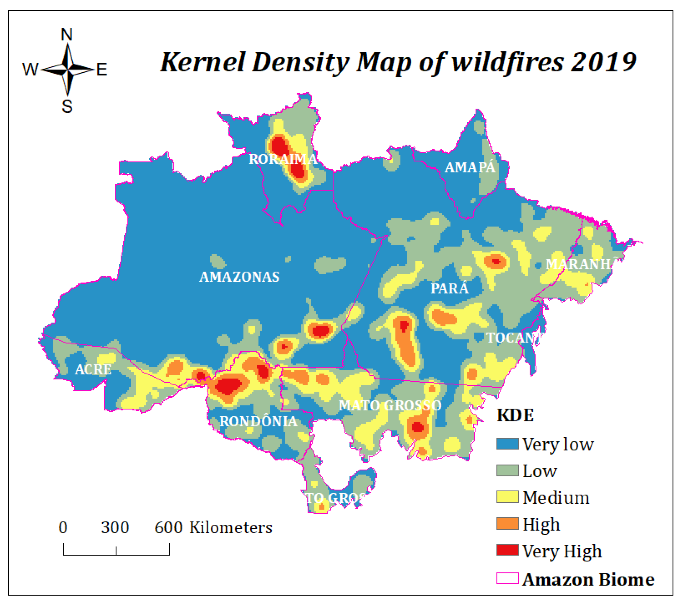
The density surface can provide a way to visualize the concentration of wildfire occurrences. As seen in Figure 4, wildfires were mainly concentrated in the northern part of Rondônia, the southern part of Amazonas, eastern Acre, and most of the central part of Roraima. In addition, there were certain degrees of aggregation in the northeast and southwest parts of Pará and the southeast part of Mato Grosso. The critical value (z-score = 159.64) in Moran’s I was greater than 2.58; there was less than a 1% likelihood that the clustered pattern is a result of a random chance, and the p-value was statistically significant. This result suggested that the pattern of wildfires at each feature location is clustered.

Figure 4.
Kernel density map of wildfire incidents in Amazônia Biome in 2019.
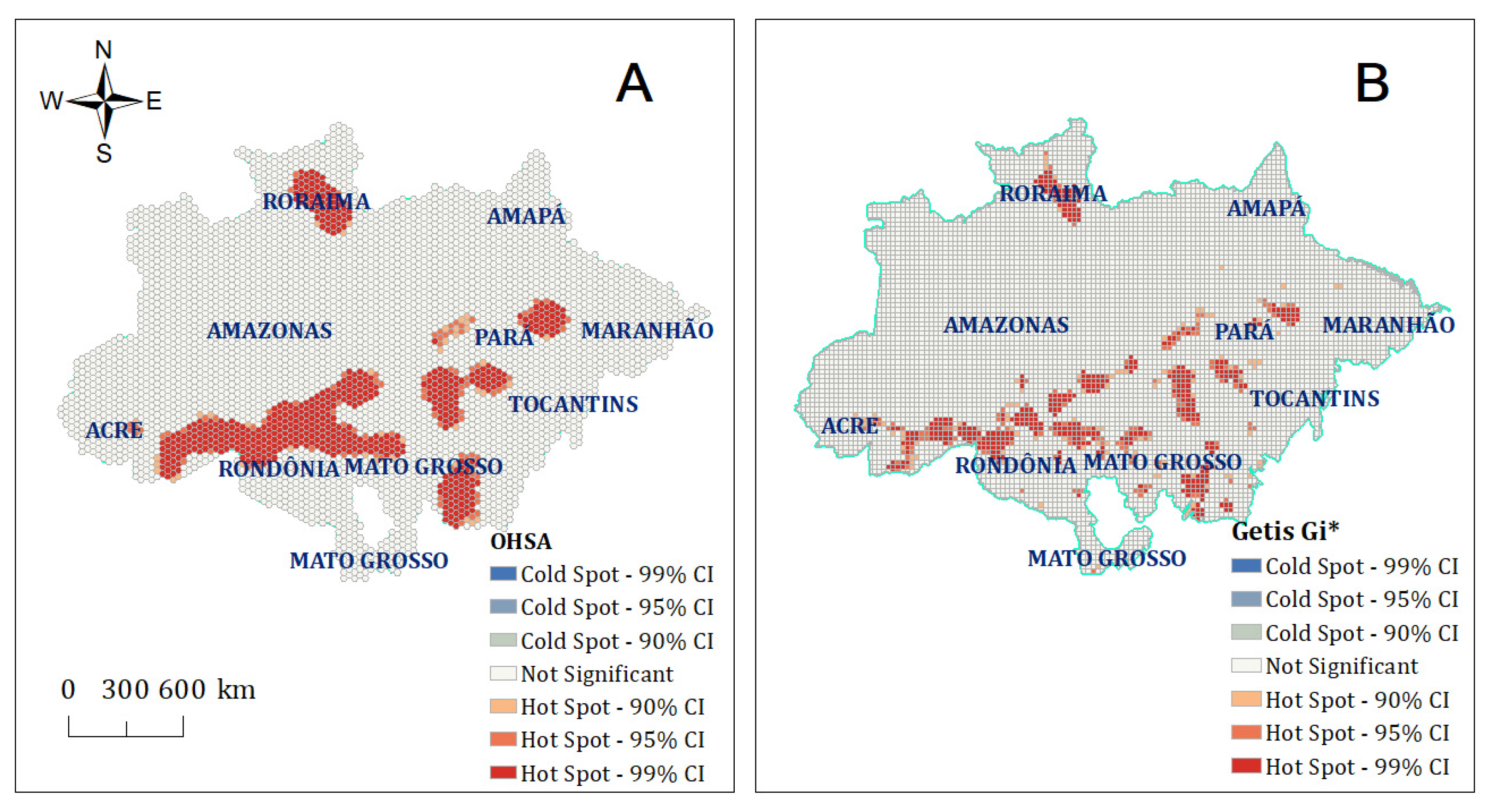
The visualized results of the OHSA and Getis-Ord Gi* for wildfires are shown in Figure 5. Figure 5A shows six hotspots with different levels of significance; one was the central part of Romania; one hotspot was related to the four states in the southwest part of the Amazônia Biome region, which comprise the states of Acre, Amazonas, Rondônia, and Mato Grosso; one was in the southeastern part of Mato Grosso; remaining three hotspots filled in the central part of Pará state. However, no cold spots had been identified, and the rest of the states were classified as “Not Significant,” which means the wildfires that occurred in those areas were distributed randomly and there were no significant patterns. By comparing the two results, the Optimized Hot Spot result (Figure 5A) indicates large hot spots that occurred over all or nearly all states. The Getis-Ord Gi* result (Figure 5B) indicates smaller, more refined hot spots that are typically distributed over sections of states.
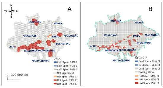
Figure 5.
Hotspot analysis. (A) OHSA in the hexagon grids, (B) Getis-Ord Gi* hotspot analysis in the fishnet grids.
4.2. Spatial Statistical Regression Analyses
4.2.1. Benchmark Regression Analysis
Before performing the GWR regression analysis, we first applied global OLS regression, in an attempt to explain the global relations between dependent and explanatory variables. The diagnoses of an OLS model indicated that all fifteen variables passed the test for multicollinearity. It explained about percent (adjusted R2 = 0.516) of the variation in wildfire occurrence with AICc = 20929.89. These explanatory variables were significant at a 95% confidence level ( = 0.05). The OLS model showed that elevation, slope, aspect, number of forest patches, edge proportion, population density, road density, forest loss, cropland area, pastureland area, and wind speed were significantly correlated with the wildfire counts (Table 2). In addition, the chi-squared value (1419.04) of the Koenker statistic was statistically significant. Therefore, the null hypothesis was rejected and there was a nonstationary condition in the model. The Jarque-Bera statistic returned a significant chi-squared value (p-values < 0.01), showing that the residuals were spatially clustered at a 99% confidence level and that a biased model was obtained. These results revealed that in the OLS model, the relationship between the dependent variable and the explanatory variables had spatial heterogeneity, and the GWR (GWGR and GWPR) models would be a more desirable choice.

Table 2.
OLS diagnostics statistics.
4.2.2. Geographically Weighted Gaussian Regression
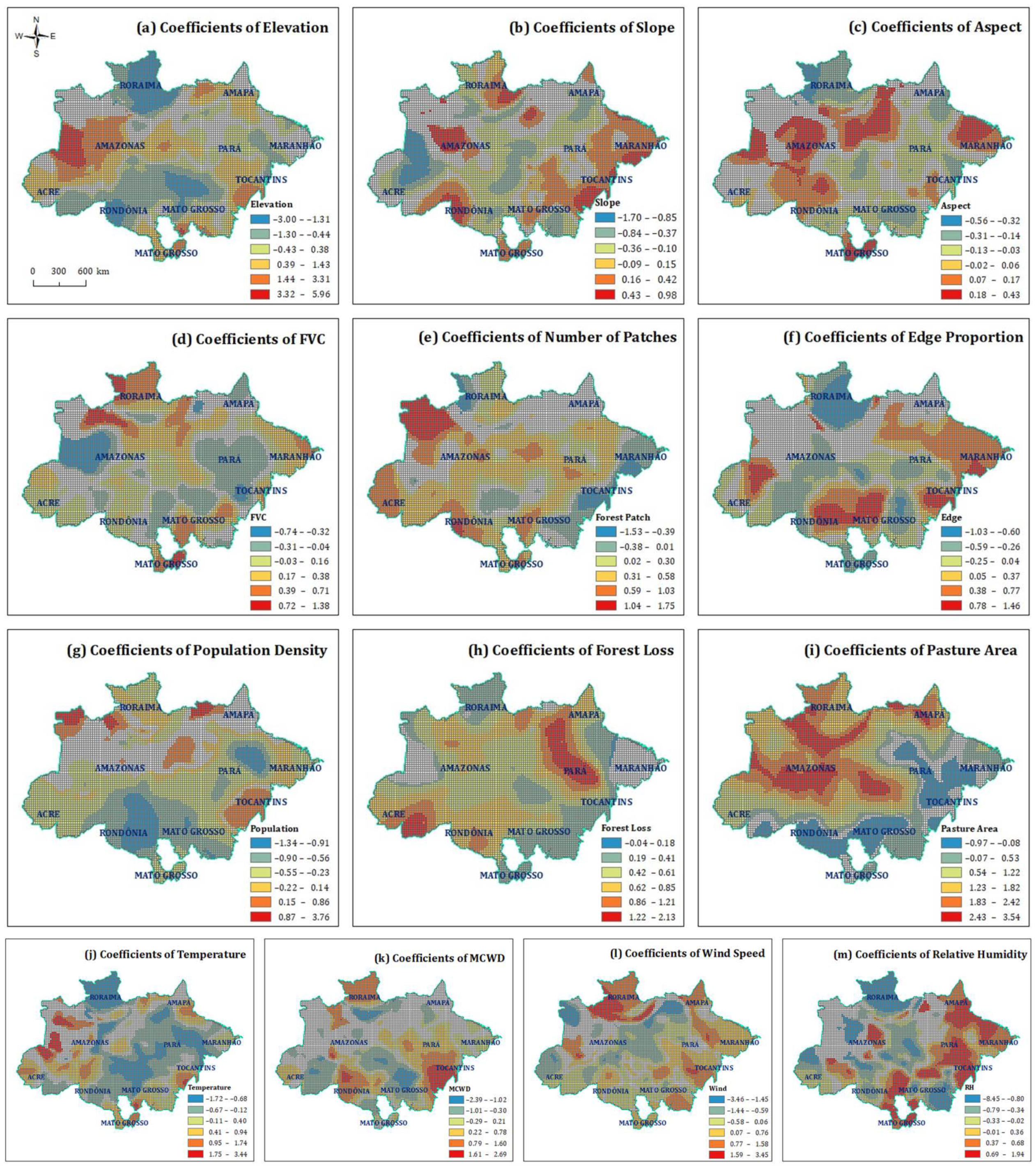
The Global Moran’s I analysis was used to determine the spatial autocorrelation of OLS and GWGR regression. By comparison, the result of Global Moran’s indicated that the residuals of OLS exhibited significant spatial autocorrelation, while the pattern of the residual from the GWGR model was random. Based on a 95% confidence level used in this study, a simple mapping technique that combines the local parameter estimates with local t-values on one map was used, in which the local t-values ranging from −1.96 to +1.96 (nonsignificant parameters) are shown in gray, whereas the significant parameters were set to 100% transparency (Figure 6).
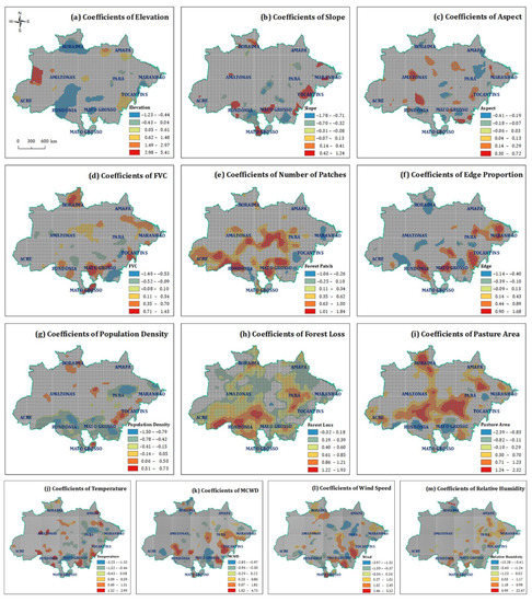
Figure 6.
Spatial distribution of significant model coefficients of GWGR. (a) Elevation, (b) Slope, (c) Aspect, (d) FVC, (e) Number of Forest Patches, (f) Edge Proportion, (g) Population Density, (h) Forest Loss, (i) Pasture Area, (j) Temperature, (k) Maximum Cumulative Water Deficit, (l) Wind Speed, (m) Relative Humidity.
For the GWGR models, the elevation is negatively correlated with wildfire occurrence in the south of Amazonas, southwest of Pará, west of Rondônia, and most areas of Roraima; the number of patches, edge proportion, forest loss, and the pastureland area were important driving factors in central Rondônia, southeastern Amazonas, central Pará, and northwestern Mato Grosso; the population density negatively impacted on wildfire occurrences in the most areas of Rondônia and northeast of Pará. Though other driving factors had a local important relationship with the wildfire occurrences, they were scattered across the study area without a recognizable pattern or clear trends.
4.2.3. Geographically Weighted Poisson Regression
Table 3 summarizes coefficient estimates and standard errors for Poisson and quasi-Poisson. Overdispersion was evident by analyzing the reported standard errors. While the Poisson and quasi-Poisson models had the same estimated regression coefficients, quasi-Poisson’s coefficient standard errors were larger. This is evidence of overdispersion and is indicated as an underestimation of standard errors by the Poisson model. Compared to the naive Poisson model, the elevation, aspect, FVC, road density, and temperature were not significant in the quasi-Poisson.

Table 3.
Poisson and quasi-Poisson diagnostics statistics.
For GWGR and GWPR models, coefficients for all explanatory variables have spatial heterogeneity, because their interquartile range (IQR) was larger two times than the standard of the global models (Table 4), which indicates certain spatial variability in the GWGR and GWPR models. In addition, we constructed the spatial maps of the local model coefficients for each explanatory variable of the GWPR models. Our results suggest that the spatial distributions of the significant model coefficients of explanatory variables between GWGR and GWPR had a certain similarity (Figure 6 and Figure 7) in the influencing direction and power.

Table 4.
Summary statistics for estimated local coefficients from the OLS and Poisson model and relative spatial variation status.
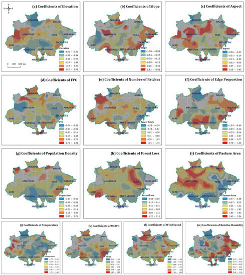
Figure 7.
Spatial distribution of significant model coefficients of GWPR. (a) Elevation, (b) Slope, (c) Aspect, (d) FVC, (e) Number of Forest Patches, (f) Edge Proportion, (g) Population Density, (h) Forest Loss, (i) Pasture Area, (j) Temperature, (k) Maximum Cumulative Water Deficit, (l) Wind Speed, (m) Relative Humidity.
For the GWPR models, the wildfire occurrences were significantly negatively related to the elevation in the west of Rondônia and central of Mato Grosso, whereas the elevation is positively correlated with wildfire occurrence in most of the Amazonas. The slope is positively related to the wildfire occurrence in the southeast of Roraima, central Amazonas, west of Rondônia, and the eastern part of the study area, including Maranhão and Tocantins. The wildfire occurrences were significantly positively related to the aspect index in most areas of Amazonas and Maranhão, south of Mato Grosso, and north of Rondônia.
For the vegetation cover and land use factors, the FVC index was mainly positively related to the wildfire occurrences in the north of Roraima, and south of Mato Grosso. The number of forest patches was positively associated with wildfire occurrences in the northwest of Amazonas and Acre, most areas of Rondônia, central Mato Grosso, and south of Pará. The edge proportion was positively related to the wildfire occurrences in the southwest of Amazonas, east of Rondônia, west of Mato Grosso, and southeast and the northeast corner of Pará, but negatively in the central and southeast of Roraima.
The population density was negatively correlated with the wildfire occurrences in most areas of Rondônia and northeast of Pará. The forest loss has significant influences on most areas of the study area; it was more predominant in the east of Acre, central Rondônia, and central and north of Pará. The pastureland area showed the different relationships with the wildfire occurrences between the northwest and southeast.
All four meteorological explanatory variables have certain degrees of correlation with wildfire occurrence across the majority of the Amazônia Biome. In general, the temperature was negatively correlated with wildfire occurrences in the northern, east-central, and south-central parts of the study area. The MCWD index positively affected the wildfire occurrences in most areas of Roraima, Rondônia, Tocantins, and south of Pará. The wind speed played a positive role in most areas of Roraima. The relative humidity negatively correlated with wildfire occurrences in most areas of Roraima and east of Mato Gross, but positive in most of the eastern part of the whole study area.
4.3. Model Evaluation and Comparison
The calibrated local model results indicate that it is a significant improvement on the global model. The adjusted R2 values of the OLS and global Poisson regression model were 0.516 and 0.550, respectively, while the corresponding Percent Deviance Explained value for the GWGR model and GWPR model was 0.746 and 0.784, respectively. By comparing the AICc values, the AICc values were 20,929 for the OLS model and 17,069 for the Poisson model, which was greater than those of both the GWGR model (15,594) and GWPR (5183) models. GWGR model was 23% better than that of the OLS model, and the GWPR model was 23.4% better than that of the Poisson model (Table 5).

Table 5.
Comparison of the performance of the four models.
To assess the potential spatial autocorrelation, we apply Moran’s I of the residuals for all models and the results show that the Moran’s I for all models were significantly positive (Z- values > 1.96), and the model residuals of the OLS regression had a slightly higher Moran’s I, while the model residuals of local Gaussian (OLS) and Poisson models had a relatively lower Moran’s I. In general, the GWR (i.e., both GWGR and GWPR) models greatly improved the model fitting and performance over the corresponding global models and produced more desirable model residuals. Figure 8 shows the map of spatial autocorrelation of the standardized residuals calculated by the four models, respectively.

Figure 8.
The standardized residuals from (a) OLS, (b) Poisson, (c) GWGR, and (d) GWPR.
5. Discussion
In humid rainforests, spontaneous fires are rare because the intact old-growth forests can maintain a microclimate moist enough [45]. However, over the past few decades, due to a growing population and an introduction of mechanized agriculture, people have often used a method called slash-and-burn to blaze forests to expand the area of land available for ranching and agriculture in exchange for economic growth (i.e., agribusiness). It has been estimated that 5665 km2 of forest have been burned and cleared since the 1970s [46]. Moreover, the deforestation activities have also increased forest fragmentation [47], which leads the microclimate along forest edges to become drier, and then the tree mortality rate has also increased, which in turn increases fuel loads, finally turning the forest into a fire-prone system. Global models support the phenomena. The results of the global model indicate that the explanatory variables of the forest loss, number of forest patches, edge proportion, cropland area, pastureland area, population density, and wind speed were statistically significantly associated with wildfire counts. Especially, the coefficients of forest loss, pastureland area, and the number of forest patches were strongly positively associated with an increased number of wildfire occurrences. These results have also corroborated that the wildfires in the Amazon Rainforest are predominant of anthropogenic origin, and deforestation and agricultural activities are the two major factors that determine the occurrence of wildfires [16].
In contrast to global models, GWGR and GWPR models were preferred to detect local relationships, which would help us identify the geographic locations where a given dependent variable may have different influences on an explanatory variable. For example, the number of forest patches was positively associated with the wildfire occurrences in the east of Acre and Amazona, west of Pará, and central Mato Grosso, but negatively associated with the wildfire occurrences in the west of Maranhão. Similarly, the pastureland area was correlated positively with the wildfire occurrences in most parts of south Amazonas, southwest of Pará, and the central Rondônia, but to be a negative relationship in the southwest of Mato Grosso. Besides, the forest loss was positively correlated with the wildfire occurrences in the central of Pará, south of the Amazonas, southeast of the Acre, northwest and central of Mato Grosso, and most of the Rondônia. In addition, our results also indicated that wildfire occurrences for 2019 were abnormally high in Acre, Amazonas, Pará, Mato Grosso, and Rondônia, and a higher level of agricultural activity was also noted in these states than in others.
In practice, wildfire occurrence is often not directly related to topographic drivers but is indirectly affected by other drivers. Wildfires in the Amazon have been proven to have significant relations with human activities, and exhibit close spatial relations with deforestation. This is because, land with a flat slope and low elevation, it is likely to be converted to agriculture. In other words, the slope and elevation drivers strongly affect the suitability of wildfire in a given location for different land uses. The results of the global model suggest that the number of wildfire occurrences increased with lower elevations and flatter terrain. This might be because human activities (e.g., agriculture) are more likely to occur in relatively low elevations and flatter terrain, which may lead to higher wildfire risk. The findings are generally supported by GWR models. The elevation is negatively correlated with wildfire occurrence in the south of Amazonas, southwest of Pará, west of Rondônia, and most areas of Roraima. Additionally, the slope was negatively associated with the wildfire occurrence in the populated southern regions of the Rondônia, whereas the slope was positively correlated with wildfire occurrence in the eastern of the Roraima because more grassland was distributed in these areas, and when the slope is steep, the grass becomes drier and are likely to cause more fires. In addition, the global model indicates that the aspect index was positively associated with wildfire occurrence. The larger the aspect index was, the closer the region was to the north and northeast, with a larger amount of sunlight and higher temperatures, which characteristics also lead to dryer fuel and thus make it also have a higher potential for wildfire occurrence. As the FVC values of the entire Amazon Rainforest are high, this driver is not significant in global models. However, it can be seen in the GWR model that FVC values are positively correlated with central Roraima and southwestern Mato Grosso.
Moreover, this study found that wildfires tended to occur in areas with low population density. The main reason is that densely populated areas are settlement areas, and human activities are relatively concentrated and far from the forest, where human activities may reduce forest cover. On the contrary, sparsely populated areas are mostly distributed at the intersection of farmland and forest, where human activities have a greater impact on forests and are more likely to generate wildfires, which is consistent with Sturtevant’s research conclusion [48]. The finding was consistent with two GWR models that show that wildfire occurrence was negatively correlated with the densely populated southern part of the Rondônia. Many studies have also confirmed that there is a positive correlation between road networks and wildfire occurrence. However, due to the multicollinearity of road density, this study did not prove them quantitatively.
This study found that the meteorological conditions were a poor discriminant of the 2019 grid fishnet wildfire occurrence, which is consistent with Kelley et al.’s [49] research conclusion. They found that during August 2019, a correlation between an area burned by wildfires and the weather conditions in Acre and the southern Amazonas was less than 0.1, and in northern Mato Grosso was even less than 0.01. In our study, although most meteorological variables were not statistically significant to the wildfire occurrences based on the global model, they were statistically significant in some regions. For example, the GWPR models found that the MCWD and relative humidity have the same influence on wildfire occurrences in the south of Amazonas, central of Rondônia, north, and south of Mato Grosso, and most of Roraima, where dry weather conditions will result in more wildfires. A large portion of these areas is covered with pastures and grasslands, where the ground vegetation is relatively sparse to contribute substantial surface fuel loads. Therefore, a relatively moist environment may reduce the risk of wildfires. However, the situation was different in the middle and south of Pará, where the predominant vegetation cover is forest, so higher relative humidity and more precipitation would increase the surface fuel loads and exacerbate the probability of wildfires. However, the results produced by the GWGR model are scattered and have no clear pattern, making interpretation difficult.
In conclusion, human activities are the main factors determining the occurrence of wildfires, followed by topographic and meteorological, which should be considered fundamental elements in the design of wildfire prevention programs. In addition, the enforcement of mandatory regulations and the monitoring of fire activity are also important techniques for preventing wildfires, particularly in areas where a fire is a significant factor in the productive cycle.
While this study has revealed the spatial pattern and driving factors of wildfire in the Amazônia Biome, there are several limitations that require further investigation. First, the spatial scale of the study area could be a limitation, and the large study area could mask subtle nuances in local regions compared to smaller scales, but broadscale spatial analysis and statistical evaluations of wildfire occurrences serve to isolate knowledge gaps and so provide a basis for subsequent analyses at a finer scale. This methodology can be applied to other Brazilian or global regions. Second, the different scales used in this analysis could lead to different results, and this could introduce reliability, potential bias, and validity concerns, as results are modifiable. In addition, this study only analyzed the phenomena of wildfire occurrences in 2019, in our future work, we can consider more about the relationship between time series and the occurrence of wildfires, to achieve multi-scale research on wildfires. Moreover, for normalizing residual distributions, the variables with nonlinear relationships were transformed by using Natural Logarithm or BOX-COX transformation [50,51]. Typically, this kind of transformation enables an analysis to fall within its legitimate application domain and to perform reliable statistical analysis. However, when the regression residual is highly non-normally distributed, it is important to know what problems may be caused by the misspecification, which can be fully discussed in future work. As Fotheringham et al. [10] pointed out, GWR may act as a microscope by magnifying the relationship’s details, while it may also amplify any existing issues.
6. Conclusions
The analysis results indicate that there were strong regional differences in the spatial patterns of wildfires. Wildfires were found to be more frequent in six states, which include the states of Acre, Amazonas, Rondônia, Roraima, Pará, and Mato Grosso. The results of spatial relationship analyses also indicate that spatial clustering was primarily caused by anthropogenic factors (i.e., deforestation and agricultural activities), and the forest loss, pastureland area, edge proportion, and the number of forest patches were strongly positively associated with an increased number of wildfire occurrences. Therefore, the areas with intense deforestation and agricultural activities and a wildland-farmland interface are those that will require a greater need for attention from fire brigades.
The assessment of model fitting and predictions shows that the GWR models had better performance than the global models. Our results were consistent with previous studies, in non-stationarity or missing variables situations, and the local models can provide a helpful complement to the global models. Additionally, other explanatory variables (e.g., the El Niño-Southern Oscillation) could be taken into account in future studies. For instance, according to Aragão et al. [35], the Multivariate El Niño Index is a powerful indicator in evaluating the severity of seasonal drought in Amazon rainforest regions.
Overall, this study can provide a wiser and better insight into wildfire mapping, understanding, prevention, and management, and intend to contribute to the field of GIS, wildfire modeling, and spatial statistics. Our results present the spatial patterns of wildfire occurrence in the Amazônia Biome in 2019 and statistically demonstrate that spatial heterogeneity existed in wildfire occurrences. In addition, GWR models have exhibited superior fitness and proven to be more predictive than global models when modeling spatial data. Finally, this study expects to enrich research contents and methods of disciplines such as remote sensing and GIS geospatial technologies, as well as to promote the mutual advancement and development of multiple disciplines.
Author Contributions
Conceptualization, C.M. and R.P.; methodology, C.M., R.P., J.D. and H.J.; software, C.M.; validation, C.M.; formal analysis, C.M.; investigation, C.M.; resources, C.M.; data curation, C.M.; writing—original draft preparation, C.M.; writing—review and editing, C.M., R.P., J.D. and H.J.; visualization, C.M.; supervision, R.P., J.D. and H.J. All authors have read and agreed to the published version of the manuscript.
Funding
This research received no external funding.
Data Availability Statement
Wildfire data are available on MODIS’s MCD14ML global monthly fire location product (https://firms.modaps.eosdis.nasa.gov, accessed on 16 April 2021). Elevation data are available on Global 30 Arc-Second Elevation (GTOPO30) (https://www.usgs.gov/centers/eros/science/, accessed on 16 April 2021). Vegetation cover data are available on MODIS NDVI (MOD13Q1) (https://lpdaac.usgs.gov/products/mod13q1v006/, accessed on 16 April 2021). Land use data are available on MapBiomas (https://mapbiomas.org/, accessed on 16 April 2021). Population data are available on WorldPop (https://www.worldpop.org/, accessed on 16 April 2021). Forest loss data are available on PRODES/INPE Amazonia (http://terrabrasilis.dpi.inpe.br/downloads/, accessed on 16 April 2021). Temperature and wind speed data are available on TerraClimate datasets (http://www.climatologylab.org/terraclimate.html, accessed on 16 April 2021). Relative Humidity data are available on Prediction of Worldwide Energy Resources (https://power.larc.nasa.gov/, accessed on 16 April 2021). MCWD data are available on Climate Hazards Group InfraRed Precipitation datasets (https://www.chc.ucsb.edu/data/chirps, accessed on 16 April 2021).
Conflicts of Interest
The authors declare no conflict of interest.
References
- Ometto, J.P.; Aguiar, A.P.D.; Martinelli, L.A. Amazon deforestation in Brazil: Effects, drivers and challenges. Carbon Manag. 2011, 2, 575–585. [Google Scholar] [CrossRef]
- Bawa, K.S.; Markham, A. Climate Change and Tropical Forests. Trends Ecol. Evol. 1995, 10, 348–349. [Google Scholar] [CrossRef]
- Silveira, M.; Petri, C.A.; Broggio, I.S. Drivers of Fire Anomalies in the Brazilian Amazon: Lessons Learned from the 2019 Fire Crisis. Land 2020, 9, 516. [Google Scholar] [CrossRef]
- Kshetri, N.; Rojas Torres, D.C.; Besada, H.; Moros Ochoa, M.A. Big Data as a Tool to Monitor and Deter Environmental Offenders in the Global South: A Multiple Case Study. Sustainability 2020, 12, 10436. [Google Scholar] [CrossRef]
- Liu, Q.; Shan, Y.; Shu, L.; Sun, P.; Du, S. Spatial and temporal distribution of forest fire frequency and forest area burnt in Jilin Province, Northeast China. J. For. Res. 2018, 29, 1233–1239. [Google Scholar] [CrossRef]
- Wittenberg, L.; Malkinson, D. Spatio-temporal perspectives of forest fires regimes in a maturing Mediterranean mixed pine landscape. Eur. J. For. Res. 2009, 128, 297–304. [Google Scholar] [CrossRef]
- Liu, Q.; Qin, X.; Li, X. A Study of Spatiotemporal Characteristics of Forest Fires in Sichuan Province Based on Point Pattern’s Method. J. Sichuan For. Sci. Technol. 2019, 40, 6–12. [Google Scholar]
- Genton, M.G.; Butry, D.T.; Gumpertz, M.L.; Prestemon, J.P. Spatio-temporal analysis of wildfire ignitions in the St Johns River Water Management District, Florida. Int. J. Wildland Fire 2006, 15, 87. [Google Scholar] [CrossRef]
- Román-Cuesta, M.R.; Martínez-Vilalta, J. Effectiveness of protected areas in mitigating fire within their boundaries: Case study of Chiapas, Mexico. Conserv. Biol. J. Soc. Conserv. Biol. 2006, 20, 1074–1086. [Google Scholar] [CrossRef]
- Fotheringham, A.S.; Charlton, M.; Brunsdon, C. Measuring Spatial Variations in Relationships with Geographically Weighted Regression. In Recent Developments in Spatial Analysis: Spatial Statistics, Behavioral Modelling and Computational Intelligence; Fischer, M.M., Getis, A., Eds.; Springer: Berlin, Germany; London, UK, 2011; pp. 60–82. [Google Scholar]
- Koutsias, N.; Martínez, J.; Chuvieco, E.; Allgöwer, B. Modeling wildland fire occurrence in southern Europe by a geographically weighted regression approach. In Proceedings of the 5th International Workshop on Remote Sensing and GIS Applications to Forest Fire Management: Fire Effects Assessment, Zaragoza, Spain, 16–18 June 2005; Universidad de Zaragoza: Zaragoza, Spain, 2005; pp. 57–60. [Google Scholar]
- Avila-Flores, D.; Pompa-Garcia, M.; Antonio-Nemiga, X.; Rodriguez-Trejo, D.A.; Vargas-Perez, E.; Santillan-Perez, J. Driving factors for forest fire occurrence in Durango State of Mexico: A geospatial perspective. Chin. Geogr. Sci. 2010, 20, 491–497. [Google Scholar] [CrossRef]
- Parisien, M.A.; Moritz, M.A. Environmental controls on the distribution of wildfire at multiple spatial scales. Ecol. Monogr. 2009, 79, 127–154. [Google Scholar] [CrossRef]
- Morello, T.F.; Ramos, R.M.; Anderson, L.O.; Owen, N.; Rosan, T.M.; Steil, L.O.; Erson, L.; Owen, N.; Rosan, T.M.; Steil, L. Predicting fires for policy making: Improving accuracy of fire brigade allocation in the Brazilian Amazon. Ecol. Econ. 2020, 169, 106501. [Google Scholar] [CrossRef]
- Hilker, T.; Lyapustin, A.I.; Tucker, C.J.; Hall, F.G.; Myneni, R.B.; Wang, Y.; Bi, J.; Mendes de Moura, Y.; Sellers, P.J. Vegetation dynamics and rainfall sensitivity of the Amazon. Proc. Natl. Acad. Sci. USA 2014, 111, 16041–16046. [Google Scholar] [CrossRef] [PubMed]
- Silva, C.H.L.; Aragão, L.E.; Fonseca, M.G.; Almeida, C.T.; Vedovato, L.B.; Anderson, L.O. Deforestation-Induced Fragmentation Increases Forest Fire Occurrence in Central Brazilian Amazonia. Forests 2018, 9, 305. [Google Scholar] [CrossRef]
- Devisscher, T.; Anderson, L.O.; Aragão Luiz, E.O.C.; Galván, L.; Malhi, Y. Increased Wildfire Risk Driven by Climate and Development Interactions in the Bolivian Chiquitania, Southern Amazonia. PLoS ONE 2016, 11, e0161323. [Google Scholar] [CrossRef]
- Schulte, L.A.; Mladenoff, D.J. Severe wind and fire regimes in northern forests: Historical variability at the regional scale. Ecology 2005, 86, 431–445. [Google Scholar] [CrossRef]
- Ali, A.A.; Carcaillet, C.; Bergeron, Y. Long-term fire frequency variability in the eastern Canadian boreal forest: The influences of climate vs. local factors. Glob. Chang. Biol. 2009, 15, 1230–1241. [Google Scholar] [CrossRef]
- Wood, S.W.; Murphy, B.P.; Bowman David, M.J.S. Firescape ecology: How topography determines the contrasting distribution of fire and rain forest in the south-west of the Tasmanian Wilderness World Heritage Area. J. Biogeogr. 2011, 38, 1807–1820. [Google Scholar] [CrossRef]
- Stage, A.R. An Expression for the Effect of Aspect, Slope, and Habitat Type on Tree Growth. For. Sci. 1976, 22, 457–460. [Google Scholar]
- Alencar, A.; Nepstad, D.; Diaz, M.C.V. Forest Understory Fire in the Brazilian Amazon in ENSO and Non-ENSO Years: Area Burned and Committed Carbon Emissions. Earth Interact. 2006, 10, 1–17. [Google Scholar] [CrossRef]
- Armenteras, D.; González, T.M.; Retana, J. Forest fragmentation and edge influence on fire occurrence and intensity under different management types in Amazon forests. Biol. Conserv. 2013, 159, 73–79. [Google Scholar] [CrossRef]
- Cochrane, M.A. Synergistic Interactions between Habitat Fragmentation and Fire in Evergreen Tropical Forests. Conserv. Biol. 2001, 15, 1515–1521. [Google Scholar] [CrossRef]
- Bucini, G.; Lambin, E.F. Fire impacts on vegetation in Central Africa: A remote-sensing-based statistical analysis. Appl. Geogr. 2002, 22, 27–48. [Google Scholar] [CrossRef]
- Morton, D.C.; Defries, R.S.; Randerson, J.T.; Giglio, L.; Schroeder, W.; van Der Werf, G.R. Agricultural intensification increases deforestation fire activity in Amazonia. Glob. Chang. Biol. 2008, 14, 2262–2275. [Google Scholar] [CrossRef]
- Marlon, J.R.; Bartlein, P.J.; Carcaillet, C.; Gavin, D.G.; Harrison, S.P.; Higuera, P.E.; Joos, F.; Power, M.J.; Prentice, I.C. Climate and human influences on global biomass burning over the past two millennia. Nat. Geosci. 2008, 1, 697–702. [Google Scholar] [CrossRef]
- Schelhaas, M.-J.; Hengeveld, G.; Moriondo, M.; Reinds, G.J.; Kundzewicz, Z.W.; Maat, H.; Bindi, M. Assessing risk and adaptation options to fires and windstorms in European forestry. Mitig. Adapt. Strat. Glob. Chang. 2010, 15, 681–701. [Google Scholar] [CrossRef]
- San-Miguel-Ayanz, J.; Moreno, J.M.; Camia, A. Analysis of large fires in European Mediterranean landscapes: Lessons learned and perspectives. For. Ecol. Manag. 2013, 294, 11–22. [Google Scholar] [CrossRef]
- Westerling, A.L.; Hidalgo, H.G.; Cayan, D.R.; Swetnam, T.W. Warming and earlier spring increase western U.S. forest wildfire activity. Science 2006, 313, 940–943. [Google Scholar] [CrossRef]
- Flannigan, M.D.; Krawchuk, M.A.; Groot, W.J.d.; Wotton, B.M.; Gowman, L.M. Implications of changing climate for global wildland fire. Int. J. Wildland Fire 2009, 18, 483. [Google Scholar] [CrossRef]
- Wotton, B.M.; Nock, C.A.; Flannigan, M.D. Forest fire occurrence and climate change in Canada. Int. J. Wildland Fire 2010, 19, 253. [Google Scholar] [CrossRef]
- Živanović, S.; Ivanović, R.; Nikolić, M.; Đokić, M.; Tošić, I. Influence of air temperature and precipitation on the risk of forest fires in Serbia. Meteorol. Atmos. Phys. 2020, 132, 869–883. [Google Scholar] [CrossRef]
- Beer, T. The interaction of wind and fire. Bound. Layer Meteorol. 1991, 54, 287–308. [Google Scholar] [CrossRef]
- Aragão, L.E.O.C.; Malhi, Y.; Roman-Cuesta, R.M.; Saatchi, S.; Anderson, L.O.; Shimabukuro, Y.E. Spatial patterns and fire response of recent Amazonian droughts. Geophys. Res. Lett. 2007, 34(7), L07701. [Google Scholar] [CrossRef]
- Gavin, J.; Haberman, S.; Verrall, R. Moving weighted average graduation using kernel estimation. Insur. Math. Econ. 1993, 12, 113–126. [Google Scholar] [CrossRef]
- Silverman, B.W. Density Estimation for Statistics and Data Analysis; CRC Press: Boca Raton, FL, USA, 2018. [Google Scholar]
- Koutsias, N.; Kalabokidis, K.D.; Allgöwer, B. Fire occurrence patterns at landscape level: Beyond positional accuracy of ignition points with kernel density estimation methods. Nat. Resour. Model. 2004, 17, 359–375. [Google Scholar] [CrossRef]
- Tomaszewski, B. Geographic Information Systems (GIS) for Disaster Management; Routledge: New York, NY, USA, 2021. [Google Scholar]
- Haining, R.; Law, J.; Griffith, D. Modelling small area counts in the presence of overdispersion and spatial autocorrelation. Comput. Stat. Data Anal. 2009, 53, 2923–2937. [Google Scholar] [CrossRef]
- Dayananda, P. Stochastic models for forest fires. Ecol. Model. 1977, 3, 309–313. [Google Scholar] [CrossRef]
- Cameron, A.C.; Trivedi, P.K. Regression Analysis of Count Data; Cambridge University Press: Cambridge, UK, 2013. [Google Scholar]
- Ismail, N.; Jemain, A.A. Handling overdispersion with negative binomial and generalized Poisson regression models. Casualty Actuar. Soc. Forum 2007, 2007, 103–158. [Google Scholar]
- Lee, J.-H.; Han, G.; Fulp, W.J.; Giuliano, A.R. Analysis of overdispersed count data: Application to the Human Papillomavirus Infection in Men (HIM) Study. Epidemiol. Infect. 2012, 140, 1087–1094. [Google Scholar] [CrossRef]
- Stewart, M. An Analysis of Amazonian Forest Fires. Available online: https://towardsdatascience.com/an-analysis-of-amazonian-forest-fires-8facca63ba69 (accessed on 21 September 2020).
- Butler, R.A. The Amazon Rainforest. Available online: https://rainforests.mongabay.com/amazon/ (accessed on 10 April 2022).
- Soares-Filho, B.; Silvestrini, R.; Nepstad, D.; Brando, P.; Rodrigues, H.; Alencar, A.; Coe, M.; Locks, C.; Lima, L.; Hissa, L.; et al. Forest fragmentation, climate change and understory fire regimes on the Amazonian landscapes of the Xingu headwaters. Landscape Ecol. 2012, 27, 585–598. [Google Scholar] [CrossRef]
- Sturtevant, B.R.; Cleland, D.T. Human and biophysical factors influencing modern fire disturbance in northern Wisconsin. Int. J. Wildland Fire 2007, 16, 398. [Google Scholar] [CrossRef]
- Kelley, D.I.; Burton, C.; Huntingford, C.; Brown, M.A.J.; Whitley, R.; Dong, N. Technical note: Low meteorological influence found in 2019 Amazonia fires. Biogeosciences 2021, 18, 787–804. [Google Scholar] [CrossRef]
- Box, G.E.P.; Cox, D.R. An Analysis of Transformations. J. R. Stat. Soc. Ser. B Methodol. 1964, 26, 211–243. [Google Scholar] [CrossRef]
- Faraway, J.J. Practical Regression and ANOVA Using R. Available online: http://csyue.nccu.edu.tw/Practical%20Regression%20and%20Anova%20using%20R.pdf (accessed on 10 April 2022).
Publisher’s Note: MDPI stays neutral with regard to jurisdictional claims in published maps and institutional affiliations. |
© 2022 by the authors. Licensee MDPI, Basel, Switzerland. This article is an open access article distributed under the terms and conditions of the Creative Commons Attribution (CC BY) license (https://creativecommons.org/licenses/by/4.0/).


