Communication

OpenForecast: An Assessment of the Operational Run in 2020–2021

State Hydrological Institute, 199004 Saint Petersburg, Russia
*
Author to whom correspondence should be addressed.
Geosciences 2022, 12(2), 67; https://doi.org/10.3390/geosciences12020067
Submission received: 23 December 2021 / Revised: 25 January 2022 / Accepted: 27 January 2022 / Published: 1 February 2022
(This article belongs to the Collection Early Career Scientists’ (ECS) Contributions to Geosciences)

Abstract

:
OpenForecast is the first openly available national-scale operational runoff forecasting system in Russia. Launched in March 2020, it routinely provides 7-day ahead predictions for 834 gauges across the country. Here, we provide an assessment of the OpenForecast performance on the long-term evaluation period from 14 March 2020 to 31 October 2021 (597 days) for 252 gauges for which operational data are available and quality-controlled. Results show that OpenForecast is a robust system based on reliable data and solid computational routines that secures efficient runoff forecasts for a diverse set of gauges.

1. Introduction

Floods remain the primary source of economic and human losses among all natural disasters [1,2,3]. During the past few decades, floods caused thousands of deaths and billions of dollars of material damage [4]. The modern trend towards warming and hence more extreme climate [5,6,7], as well as the growing anthropogenic load on the environment [8,9], leaves floods in the strong research focus as dominant impact-relevant events [5,6,10].
Continuous development and benchmarking of operational flood forecasting services are among the most dynamic research areas based on the highest relevance of early warnings for prevention of disastrous flood events and reduction of their impacts [11,12]. Today, many forecasting services—from global [13,14,15] to continental [16,17,18,19], national [20,21,22], and regional scales [23,24,25]—are in operational use, producing timely and reliable runoff forecasts. All these services are complex structures based on many individual components that provide, e.g., operational data assimilation, forecast computation, and dissemination functionality [26,27,28]. Hence, it is important to guide the directed development of operational runoff forecasting services and their components towards more skillful predictions by the continuous evaluation of their performance [29].
OpenForecast is the first national-scale operational runoff forecasting system in Russia [20,24] that has been developed since 2018 by the consortium of researchers from the State Hydrological Institute (Saint-Petersburg, Russia), the Water Problems Institute (Moscow, Russia), the Central Administration for Hydrometeorology and Ecology Monitoring (Moscow, Russia), and the Lomonosov Moscow State University (Moscow, Russia) on the funds provided by the Russian Foundation for Basic Research. The system was launched on 14 March 2020. Since then, OpenForecast operationally provided one week ahead runoff forecasts for 843 gauges across Russia. In our previous research studies, we presented: (1) the proof of concept of runoff forecasting service design (OpenForecast v1 [24]) that has been evaluated for three pilot river basins in the European part of Russia for the period from 1 March 2019 to 30 April 2019 (61 days), and (2) the second version of the OpenForecast system (OpenForecast v2 [20]) that has been scaled to 834 gauges across Russia and then evaluated for the period from 14 March 2020 to 6 July 2020 (115 days). Both studies confirmed OpenForecast as a successful example of the state-of-the-art national-scale runoff forecasting system. However, short evaluation periods leave room for speculation about the system’s consistency and robustness.
Here, in this Short Communication, we aim to provide a long-term assessment of the OpenForecast performance metrics based on the results obtained for the period from 14 March 2020 to 31 October 2021 (597 days). There are five central research questions:
  • Is there a consistency between the performance on calibration and evaluation periods?
  • Is there a consistency between the performance of computed runoff hindcasts and forecasts? What are the differences in performance between distinct hydrological models?
  • Is communicating ensemble mean a good strategy for forecast dissemination?
  • What is the role of meteorological forecast efficiency in runoff forecasting?
  • How many people do use OpenForecast?
In our opinion, even a brief investigation of the research questions mentioned above would increase the confidence in OpenForecast’s reliability among the general audience, academic, and government institutions.

2. Data and Methods

The comprehensive description of data and methods used for the development of the OpenForecast system is provided in an open-access paper [20]. Here, we briefly introduce the system’s main underlying data sources and computational components required to support results presentation and analysis.

2.1. Runoff Data

Streamflow and water level observations for the historical period (2008–2017) are available at the website of the Automated Information System for State Monitoring of Water Bodies (AIS; https://gmvo.skniivh.ru, accessed on 10 December 2021). Streamflow (m3/s) observations have been used for hydrological model calibration. In addition to streamflow, water level (cm above the “gauge null”) observations have been used to calculate rating curves for the transformation of streamflow values to water level (and vice versa) for the corresponding gauges.
Only water level observations for a limited number of gauges are available operationally at the Unified State System of Information website regarding the Situation in the World Ocean (ESIMO; http://esimo.ru/dataview/viewresource?resourceId=RU_RIHMI-WDC_1325_1, accessed on 10 December 2021).

2.2. Meteorological Data

ERA5 global meteorological reanalysis [30] and its pre-operational (5 day delay from the real-time) product ERA5T serves as a source of historical meteorological forcing of air temperature (T, °C) and precipitation (P, mm). The outputs from the global numerical weather prediction model ICON [31] serve as a source of deterministic 7 day-ahead meteorological forecasts for air temperature and precipitation. Here, meteorological data have been aggregated to the daily time step and then averaged at the basin scale for each available river basin. In addition to air temperature and precipitation, potential evaporation ( P E , mm) is calculated using the temperature-based equation proposed in [32].

2.3. Hydrological Models

We use two conceptual lumped hydrological models: HBV [33], and GR4J [34]. While HBV has an internal snow module, the GR4J model has been complemented with the Cema–Neige snow accumulation routine [35,36]. Both models require only daily precipitation, air temperature, and potential evaporation as inputs (see Section 2.2). HBV and GR4J models have 14 and six free parameters, respectively (Table 1 and Table 2).
For each available river basin, model parameters have been automatically calibrated against observed runoff using two loss functions: (1) the Nash–Sutcliffe efficiency coefficient (NSE; Equation (1); [37]) and (2) the Kling–Gupta efficiency coefficient (KGE; Equation (2); [38]). Here, utilization of different loss functions is the simplest way to introduce an ensemble approach for runoff forecasting [39]. Thus, in the OpenForecast system, there are four models used to calculate runoff: H B V N S E , H B V K G E , G R 4 J N S E , and G R 4 J K G E .
N S E = 1 Ω ( Q s i m Q o b s ) 2 Ω ( Q o b s Q o b s ¯ ) 2
K G E = 1 ( r 1 ) 2 + ( σ s i m σ o b s 1 ) 2 + ( Q s i m ¯ Q o b s ¯ 1 ) 2
where Ω is the period of evaluation, Q s i m and Q o b s are the simulated and observed runoff, Q s i m ¯ and Q o b s ¯ are the mean simulated and observed runoff, r is the correlation component represented by Pearson’s correlation coefficient, σ s i m and σ o b s are the standard deviations in simulations and observations. NSE and KGE are positively oriented and not limited at the bottom: a value of 1 represents a perfect correspondence between simulations and observations. NSE > 0 and KGE > −0.41 can be considered to be showing skill against the mean flow benchmark [40].

2.4. Openforecast Runoff Forecasting System

The OpenForecast system provides one week ahead runoff forecast for 843 gauges that have been selected based on calibration results and data availability [20]. The illustration of the OpenForecast computational workflow is presented in Figure 1.
First, for each gauge of interest, meteorological forcing is updated based on the latest ERA5T and ICON data (see Section 2.2). Then, the updated meteorological forcing data is used as input to four hydrological models (Section 2.3) to obtain recent runoff forecasts. Finally, the calculated forecasts are communicated on the project’s website (https://openforecast.github.io, accessed on 14 December 2021).
Figure 2 illustrates OpenForecast’s modeling phases and the corresponding input data in more detail. There are three general phases (periods): (1) hindcast, (2) pre-operational hindcast, and (3) forecast. For the hindcast phase, ERA5 and ERA5T meteorological data is utilized. That describes hindcasts as model predictions (similar to those on the calibration period) during the run time of the forecasting system. Because of the delay of ERA5T from real-time, the scheme of filling missing data between the recent ERA5T update and ICON forecast is needed. To that, we use ICON hindcasts—the past 1 day-ahead ICON forecasts [20,24]. To distinguish this phase from the hindcast phase, which utilizes ERA5-based data instead of ICON-based, we call it pre-operational hindcast (Figure 2). Finally, we use deterministic 7 day-ahead ICON forecasts to force hydrological models to provide the corresponding predictions for the forecast phase. The results of the OpenForecast operational run have been obtained for the period from 14 March 2020 to 31 October 2021 (597 days).
While we compute four realizations of runoff predictions (by the number of utilized hydrological models; Section 2.3), we communicate only the ensemble mean (hereafter ENS), and ensemble spread on the OpenForecast website (https://openforecast.github.io, accessed on 14 December 2021).

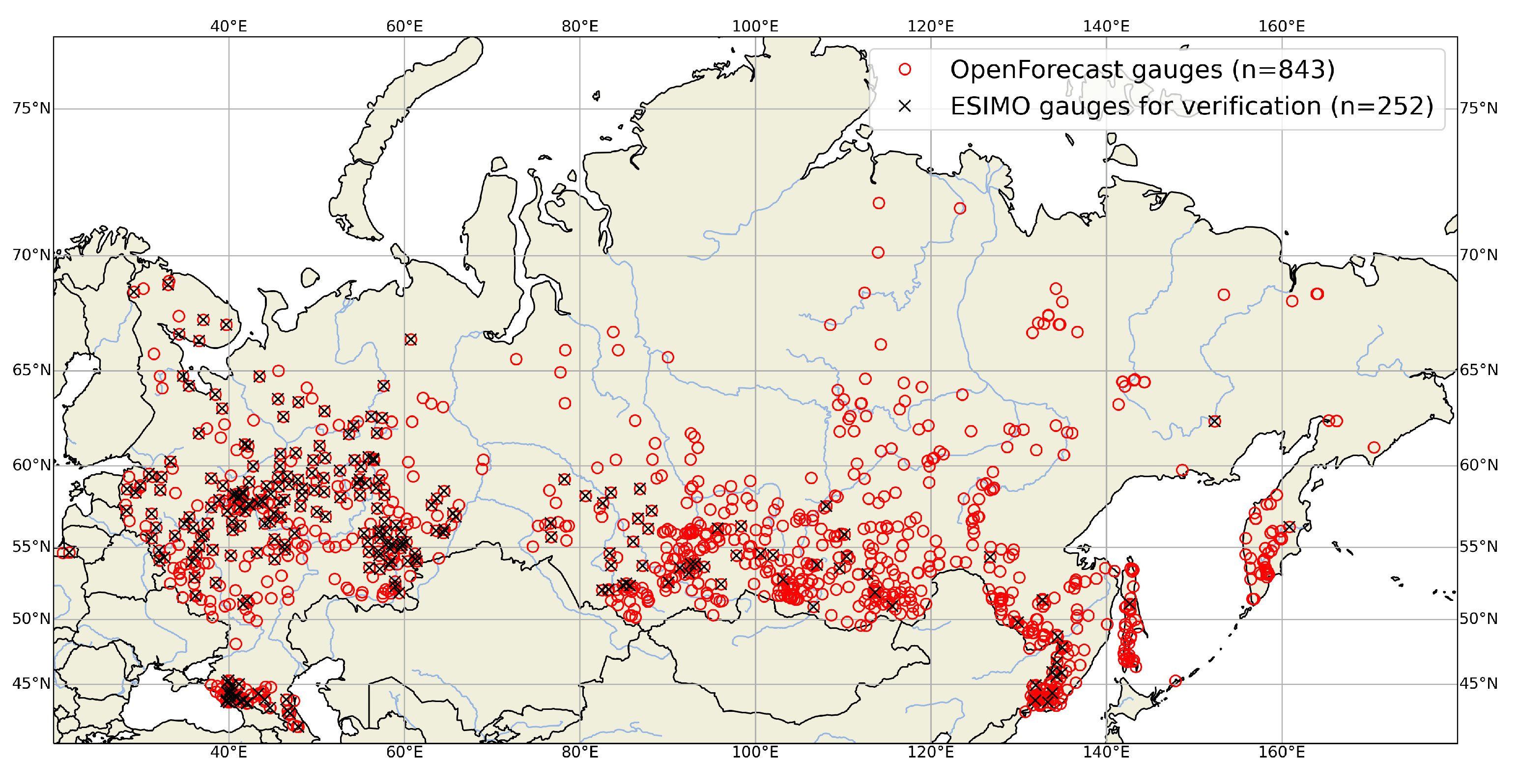
2.5. Reference Gauges

Unfortunately, it is impossible to provide an efficiency assessment of OpenForecast for each of all 834 gauges. There are two main reasons: (1) the operational information provided by the ESIMO system (Section 2.1) does not cover all OpenForecast gauges, (2) historical water level observations from the AIS system are not always consistent with operational information provided by the ESIMO. Thus, after the semi-automatic checking of operational data consistency (e.g., detection of outliers, sudden changes in flow dynamics, and the visual inspection), 252 gauges have been selected for further performance assessment (Figure 3). This number represents 30% of operational OpenForecast’s gauges and could be considered representative because they keep the distribution of small, medium, and large basins similar to the general population (834 gauges). There are 13/41/46% and 20/45/35% for small/medium/large basins and the sample and the general population.

2.6. Performance Assessment Setup

The forecasts from operational systems are typically evaluated in terms of the degree of their similarity with observations [11,20,41]. To this end, here, two efficiency metrics that are widely and mostly used in hydrological studies [40,42,43] are employed: (1) the Nash–Sutcliffe Efficiency coefficient (NSE; Equation (1); [37]) and (2) the Kling–Gupta Efficiency coefficient (KGE; Equation (2); [38]).
For each reference gauge (Figure 3), we assess individual model ( H B V N S E , H B V K G E , G R 4 J N S E , and G R 4 J K G E ) performance in terms of NSE and KGE for two periods: (1) calibration (1 January 2008–31 December 2017) and (2) evaluation (hindcast) (14 March 2020–31 October 2021). Also, we assess both individual and ensemble mean (ENS) performances for seven pre-operational hindcast ( t 7 , , t 1 days) and seven forecast ( t + 1 , , t + 7 days) lead times (Figure 2) for the entire period of evaluation (14 March 2020–31 October 2021).

3. Results and Discussion

3.1. Consistency between Calibration and Evaluation Periods

Temporal consistency of model efficiency ensures computational system robustness and confidence in the underlying routines and models [44,45,46,47]. There are many cases when that consistency could be disrupted: inconsistency of meteorological data sources between periods of consideration, significant change in runoff formation or pathways (e.g., reservoir construction), instability of model parameters, to name a few. As a result, a well-calibrated model could not provide reliable predictions under new conditions.
Here, we provide results of model efficiency assessment for two periods: (1) calibration and (2) hindcast (evaluation). Figure 4 illustrates the differences between efficiencies of the individual models in terms of NSE (see Figure A1 for the KGE metric) for 843 OpenForecast gauges. The obtained results are similar for all models and illustrate visually distinct differences between model performance on two independent periods. Expectedly, individual model efficiencies decrease on the hindcast period compared to the calibration period. The median NSE is dropped from 0.81 to 0.71, 0.78 to 0.66, 0.82 to 0.64, 0.8 to 0.63 for G R 4 J N S E , G R 4 J K G E , H B V N S E , and H B V K G E , respectively. Major quantiles, 25th and 75th, also follow the same pattern. Also, it is visually clear that the bottom “tail” of lower values is bigger on the hindcast period than on the calibration period. Here, obtained results also show that the HBV-based models with 14 calibrated parameters, H B V N S E and H B V K G E , lose more efficiency than GR4J-based models with six calibrated parameters, G R 4 J N S E and G R 4 J K G E . That provides an interesting insight into the higher reliability of simpler models for runoff forecasting even if they had comparable efficiency during the calibration period. However, that distinct decrease in performance from the calibration to the hindcast period could not be considered crucial and critical for the forecasting system’s reliability. Only the minor number of gauges show unskillful results in terms of NSE (NSE ≤ 0): four, nine, seven, and 16 for G R 4 J N S E , G R 4 J K G E , H B V N S E , and H B V K G E , respectively. Sixteen gauges with unskillful NSE for H B V K G E model include those detected for other individual models. Most of them (12 out of 16) are located in the European part of Russia and represent small and medium-size basins (under 10,000 km2). There are 58, 78, 78, and 87 gauges that show unsatisfactory (after [48]) yet skillful results in terms of NSE (NSE ≤ 0.5). However, there is no distinct pattern in their spatial or basin area distribution. In terms of KGE, unskillful results (KGE ≤ −0.41) have shown only for a single gauge by G R 4 J N S E and G R 4 J K G E models. Therefore, we argue that OpenForecast’s underlying hydrological models are robust and provide a solid basis for reliable runoff predictions.
The decrease of model efficiency on the evaluation period compared to the calibration period is commonplace in hydrological modeling studies, and well-reported in literature [20,44,45,46,47]. There are several significant reasons for that behavior, e.g., changing meteorological or landscape conditions of considered periods or/and instability of model parameters. However, for the present case of OpenForecast efficiency assessment, the factor of observational data inconsistency takes its lead. First, for the performance assessment, we use operational water level data from the ESIMO system that could be inconsistent with historical runoff data from the AIS system that we use for model calibration (Section 2.1). ESIMO’s data does not undergo correction routines, so that it could be misleading for some number of gauges. Additionally, for some gauges, processes of river channel transformation may play a huge role, so the correction of the rating curve is needed for reliable conversion of operational water levels to runoff. Unfortunately, the AIS database has a significant time lag for approximately two years of update cycles. Thus, we could provide an OpenForecast performance assessment based on consistent runoff data no earlier than the end of 2022.
Figure 5 shows the spatial distribution of differences in NSE between the calibration and hindcast periods ( N S E h i n d c a s t N S E c a l i b r a t i o n ) for the H B V K G E model for which the corresponding differences are the most pronounced. First, we should mention that for 34 gauges (13.5%), NSE on the hindcast period is higher than the calibration period. No distinct spatial clusters of plotted differences could be attributed appropriately to geographical or hydrological factors.
It was also expected that models that have been calibrated using particular metrics (either NSE or KGE) would have better results in terms of those metrics on the evaluation (hindcast period). Thus, G R 4 J N S E and H B V N S E have higher median NSE efficiencies (0.71 and 0.64, respectively) than G R 4 J K G E and H B V K G E (0.66 and 0.63, respectively) on the evaluation (hindcast) period. Obtained results raise a question of the best metric that could serve the needs of all interested parties: professional community, government agencies, and general public [49]. Currently, NSE and KGE metrics are popular only within the hydrological community. Hence, we need a targeted effort to make them (or more successful analogs) familiar to the general public.

3.2. Consistency between Hindcasts and Forecasts

In contrast to the comparison of model efficiencies between the calibration and evaluation (hindcast) periods where the general idea was to validate overall model reliability and robustness on contrasting periods (Section 3.1), here we aim to evaluate the consistency and skill of model predictions under the inconsistent input data for the hindcast, pre-operational hindcast, and forecast modeling phases (Figure 2). The difference in prediction efficiency between the hindcast and pre-operational hindcast periods aims to highlight the trade-off of the transition from the ERA5 reanalysis to ICON hindcast to fill in meteorological forcing data seven days before the forecast run time (Figure 2). The difference in prediction efficiency between the pre-operational hindcast and forecast periods describes forecasting efficiency and highlights the cumulative role of initial conditions and meteorological forecasts in efficiency decrease over lead time.
Figure 6 illustrates the distribution of individual and ensemble mean (ENS) model performances in terms of NSE for the hindcast period, as well as for seven pre-operational hindcast ( t 7 , , t 1 days) and seven forecast ( t + 1 , , t + 7 days) lead times for 252 OpenForecast gauges (see Figure A2 for the KGE metric). First, it is visually apparent that all models follow the same pattern of efficiency change: the efficiency slowly decreases with increasing lead time, and there are no significant drops between hindcast, pre-operational hindcast, and forecast periods. Thus, all models demonstrate persistent and robust behavior while assessed on a long-term period of almost two years (March 2020–October 2021). Both mean NSE and KGE (Figure 4 and Figure A1) are higher than behavioral values for all considered periods and lead times: 0.5 for NSE and 0.3 for KGE (after Knoben et al. [40]). The obtained results are in line with the previous large-scale assessments of the OpenForecast performance [20,50] that capitalizes on the robustness and reliability of the developed forecasting system.
Similar to the results obtained in Section 3.1, GR4J-based models ( G R 4 J N S E and G R 4 J K G E ) generally show higher efficiency than HBV-based models ( H B V N S E and H B V K G E ) in terms of the NSE metric. The differences are less pronounced in terms of the KGE metric. Thus, higher model complexity (of HBV-based models) does not ensure higher efficiency of runoff predictions and forecasts in the case of the OpenForecast system. While the difference in mean NSE between GR4J and HBV-based models is significant (around 10% for each lead time), they show a similar rate of around 10% for efficiency decrease with lead time. While two different hydrological models differ in catching up with the complexity of runoff formation processes, they respond similarly to changes in meteorological input forcing (from hindcasts to forecasts).

3.3. Communication of Ensemble Mean

Despite a large variety of options in communicating ensemble runoff forecasts, there is yet no consensus on what practice fits differing requirements of many parties the best [51]. From the beginning, communication of the ensemble mean and spread is the only option in the dissemination of runoff forecasts in the OpenForecast system [24]. That choice was driven by two main factors: (1) ensemble mean could provide more skillful and less biased results than each of its members [52,53], and (2) visualization of a single line is perceptually clear and easier to understand [51]. The previous assessment studies confirm that as reliable and skillful [20,50]. Figure 7 illustrates time series of simulated ensemble mean streamflow compared to observations.
Figure 8 shows the development of mean efficiencies with a lead time for individual models, as well as their ensemble mean, for the long-term evaluation period in terms of NSE and KGE. Results show that the communication of ensemble mean is the best strategy so far—ENS demonstrates higher efficiency than all individual models for all lead times in terms of both performance metrics.
Results show that communication of ensemble mean benefits more for the end-users because of perceptual clarity and the highest prediction efficiency. The latter probably is a result of a combination of structurally different yet efficient models [53,54,55]. We see ample potential to increase further the number of hydrological models within the computational core of OpenForecast. The recent advances in hydrological model distribution as an open-source software package [56,57,58] makes it particularly easy to implement and further capitalizes on the open nature of the OpenForecast system.

3.4. Role of Meteorological Forecast Efficiency

Discrepancies between observed and predicted runoff may have many sources (uncertainties), e.g., the inability of the hydrological model to capture the entire diversity of runoff formation processes on the considered watershed, and/or systematic biases in meteorological input data that could trigger errors in initial conditions and following predictions [59,60]. In the presented study, we provide information on cumulative model-related and data-induced errors that could be represented as a difference between the reference efficiency (1 for both NSE and KGE) and the efficiency on the calibration/evaluation (Section 3.1) and forecast (Section 3.2) periods. Results showed that, on average, runoff forecast efficiency decreases on 10% in terms of NSE between t 1 and t + 7 days lead times (Section 3.2, Figure 8). While it is almost impossible to distinguish the different sources of errors in runoff prediction without a controlled environment, here we provide a brief quality assessment of ICON forecasts comparing them with ERA5 data, which is considered as ground truth (Figure 9).
Results show that while numerical weather prediction made a huge step towards increasing efficiency of weather forecasts in recent decades [61], the chaotic nature of precipitation-related processes remains the main (unsolved) problem. It is clear that the efficiency of air temperature forecasting is solid and highly reliable—the lowest correlation coefficient is around 0.93 with the lowest mean value of 0.96 for a lead time of one week (Figure 9, top panel). In contrast, the mean correlation coefficient for precipitation decreases from 0.9 to 0.29 for the lead times of t + 1 and t + 7 days, respectively (Figure 9, bottom panel). However, due to a crucial role of transformation processes of water flow on a watershed (e.g., water travel time, basin memory), that distinct decrease in precipitation forecast efficiency does not directly transfer to a similar decrease in runoff forecast efficiency. Recent studies show [62,63] that modern deep learning techniques have ample potential to set new state-of-the-art results in the field of precipitation forecasting. Until then, OpenForecast may increase the number of meteorological forecasting products (apart from sole ICON) used in the system’s computational core to provide a wider range of ensemble forecasts.

3.5. OpenForecast Users

The description of runoff forecasting systems users is usually ignored in scientific literature. The high importance of any developed forecasting system is unquestionable until it helps mitigate the effect of extreme floods. However, high importance does not assure a high number of users, and we argue that this topic has high relevance for the hydrological community, which develops forecasting services.
In contrast to weather forecasts, runoff forecasts have limited temporal and spatial demand. Floods typically occur in known flood-rich periods and should be impact-relevant, i.e., affect population and material property in river valleys, to be a problem for local communities. Thus, many people do not even require any flood forecasts, which cannot be said about the weather forecasts. Figure 10 illustrates OpenForecast daily users and devices they use to access the forecasting system website (https://openforecast.github.io, accessed on 22 December 2021).
Figure 10 shows that the daily number of OpenForecast users highly correlates with flood-rich periods of spring, snowmelt-driven (March–June) and summer, rainfall-driven (June–July) flood periods. Thus, of the 12 months of the year, only four provide an interest to the public. In this way, due to continuous operational run on an everyday basis, OpenForecast demonstrates very high idle costs—that could be negligible for government-driven agencies or big tech companies but considerable for small independent research groups or startups. Also, most OpenForecast users use it from their desktops—obsolete devices in the new mobile era. There are obvious reasons for that, e.g., the absence of mobile version or application and (comparatively) slow evolving flood events that do not require frequent on-the-go updates. The absolute number of users is also meager and could be considered negligible compared to daily users of weather forecasts (millions of people). However, we know that OpenForecast is routinely utilized as an additional information source by different government authorities; thus, it indirectly delivers reliable 7-day ahead runoff forecasts for a wider audience.

4. Conclusions

The main aim of the presented Short Communication is to provide an up-to-date performance assessment of the long-term operational run of the OpenForecast system—the first national-scale service that delivers 7-day ahead runoff forecasts for 834 gauges across Russia. To that, we assess the efficiency of OpenForecast on the evaluation period from 14 March 2020 to 31 October 2021 (597 days) for 252 gauges that have been supported by reliable operational runoff observations (Figure 3). The results could be summarized following the related research questions as follows:
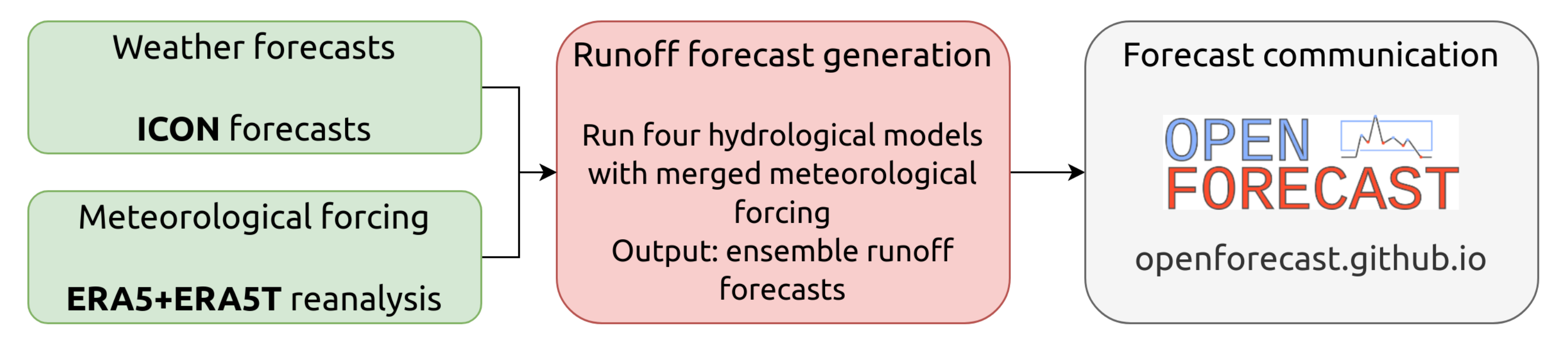
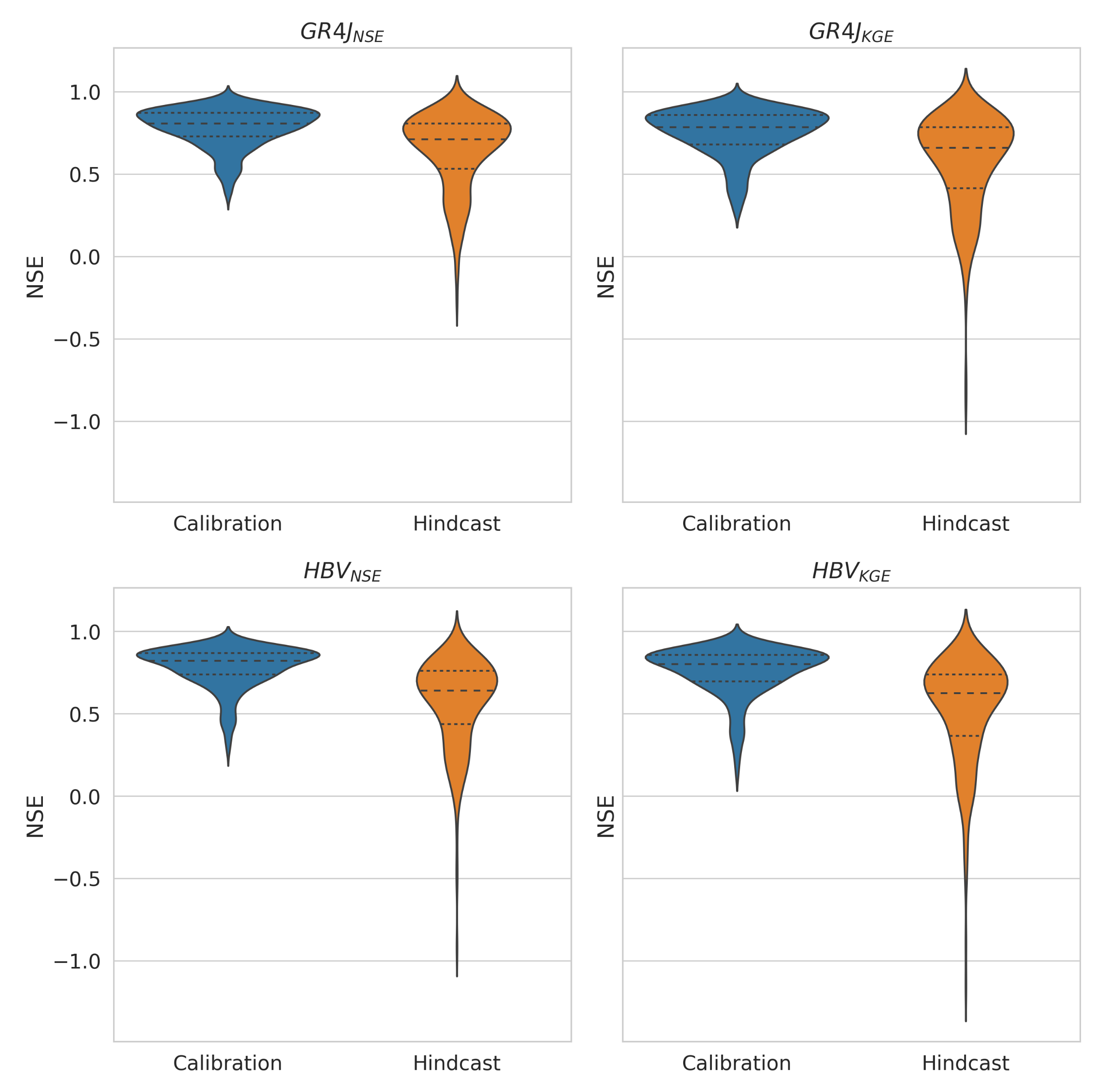
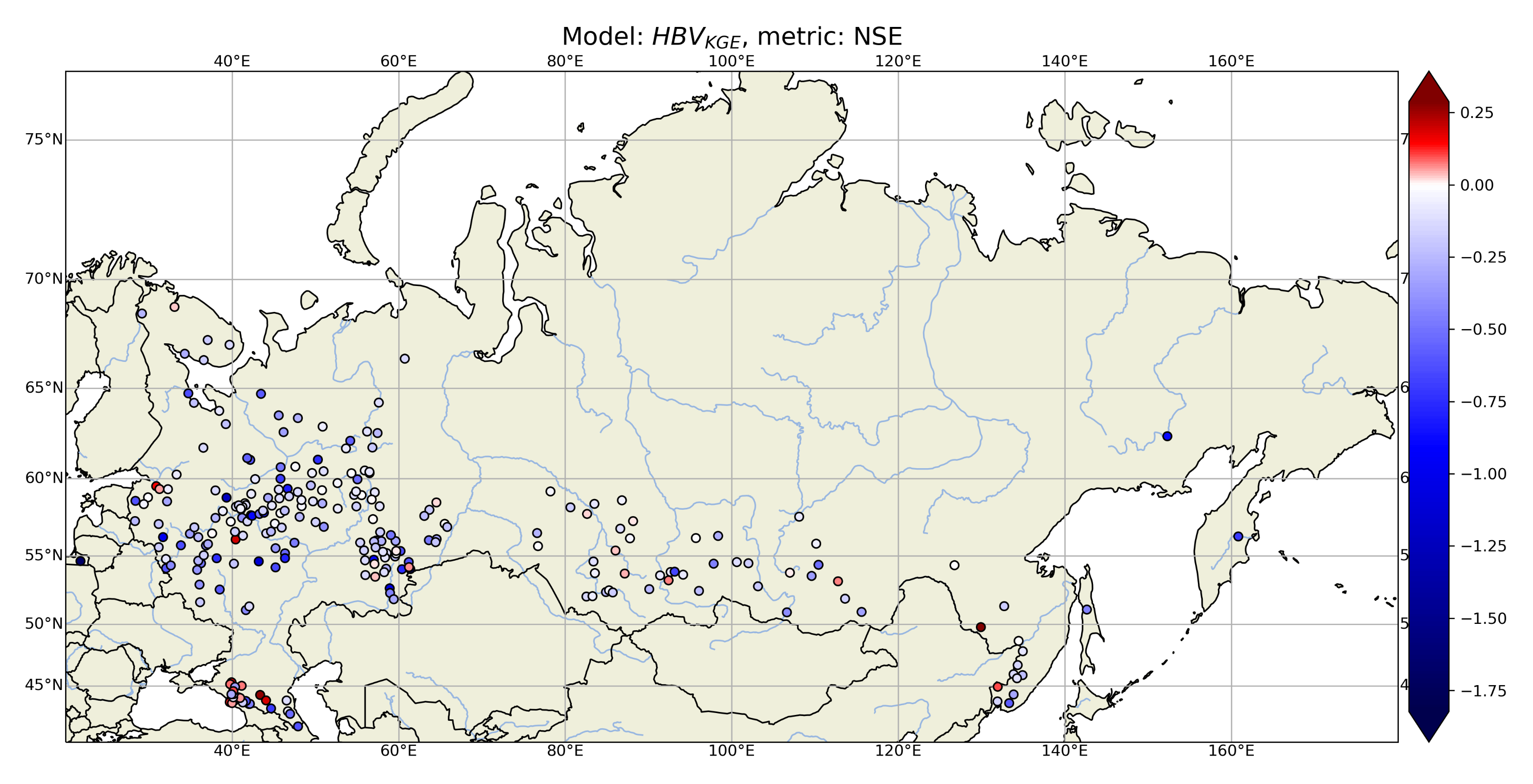
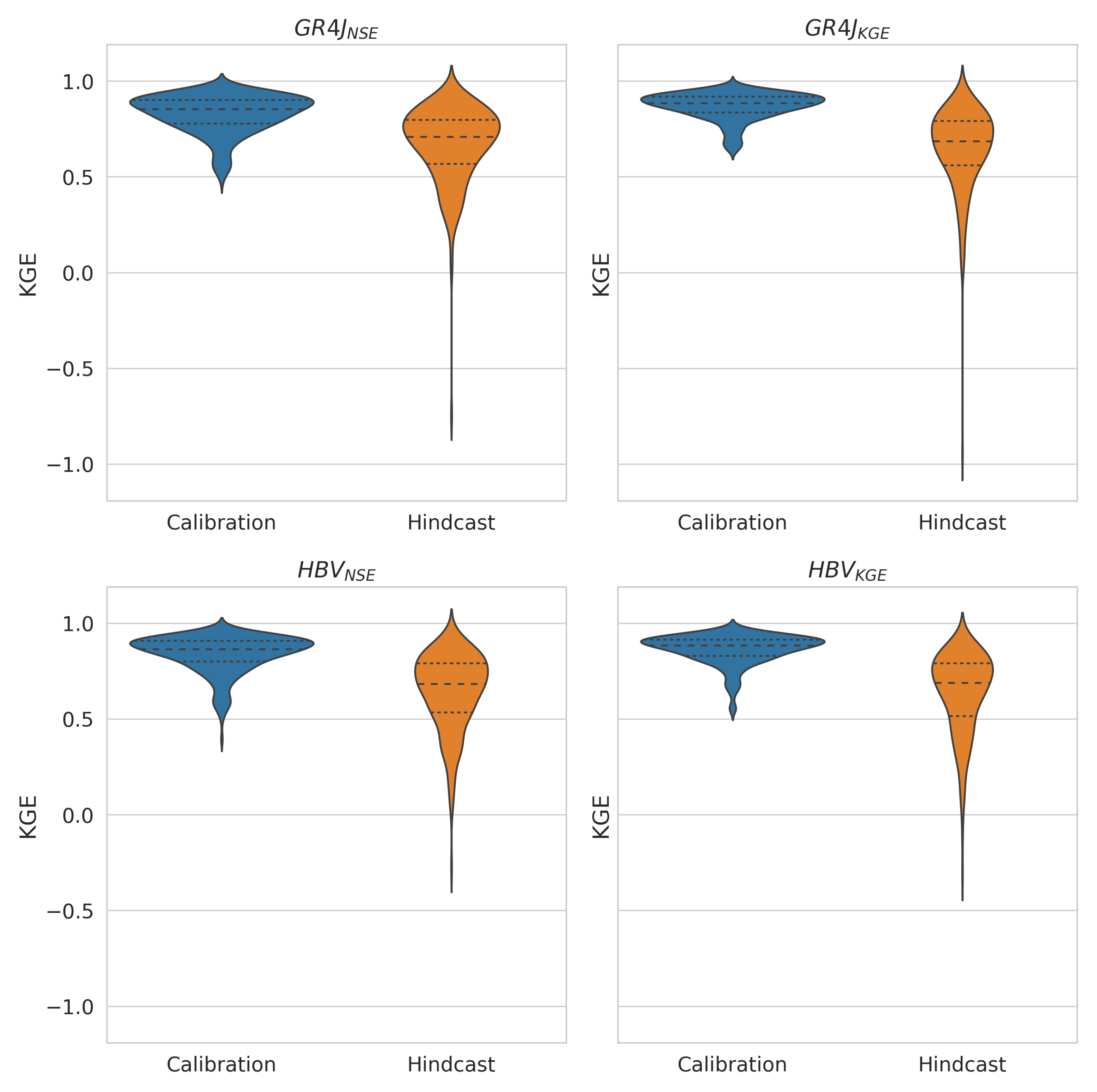
  • All hydrological models under the hood of OpenForecast computational workflow (Figure 1) demonstrate robust and reliable results of runoff prediction either on calibration or evaluation (hindcast) periods (Figure 4). We argue that the selected hydrological models form a solid basis for operational forecasting systems allowing consistent and skillful runoff predictions.
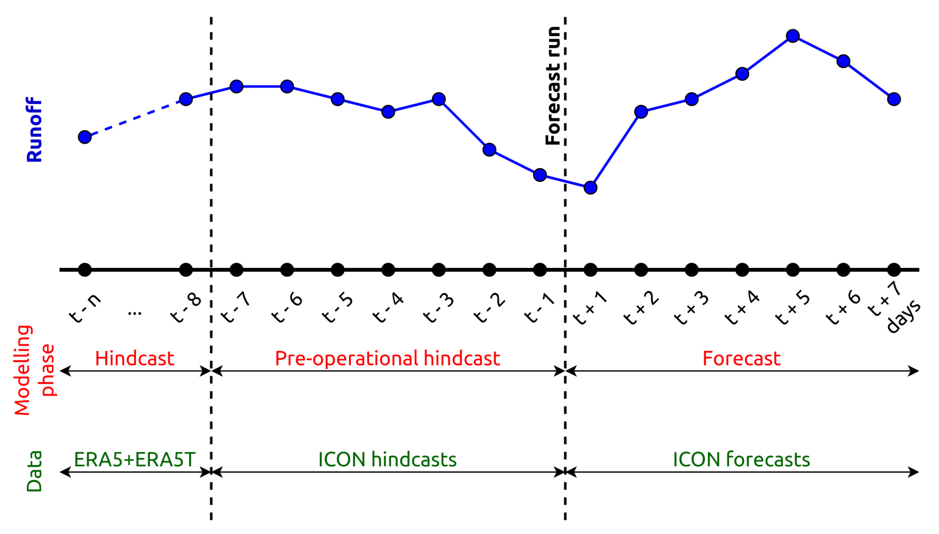
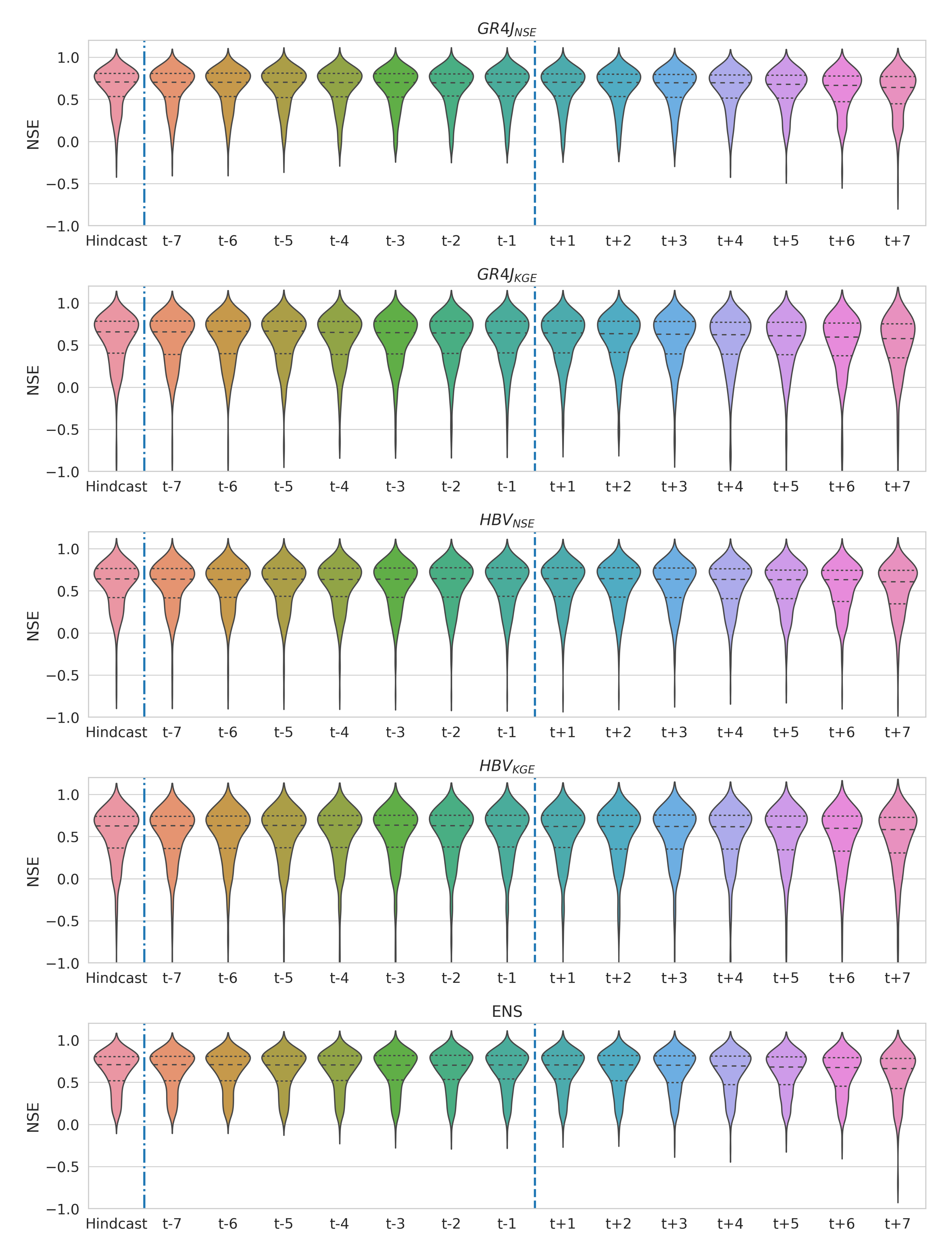
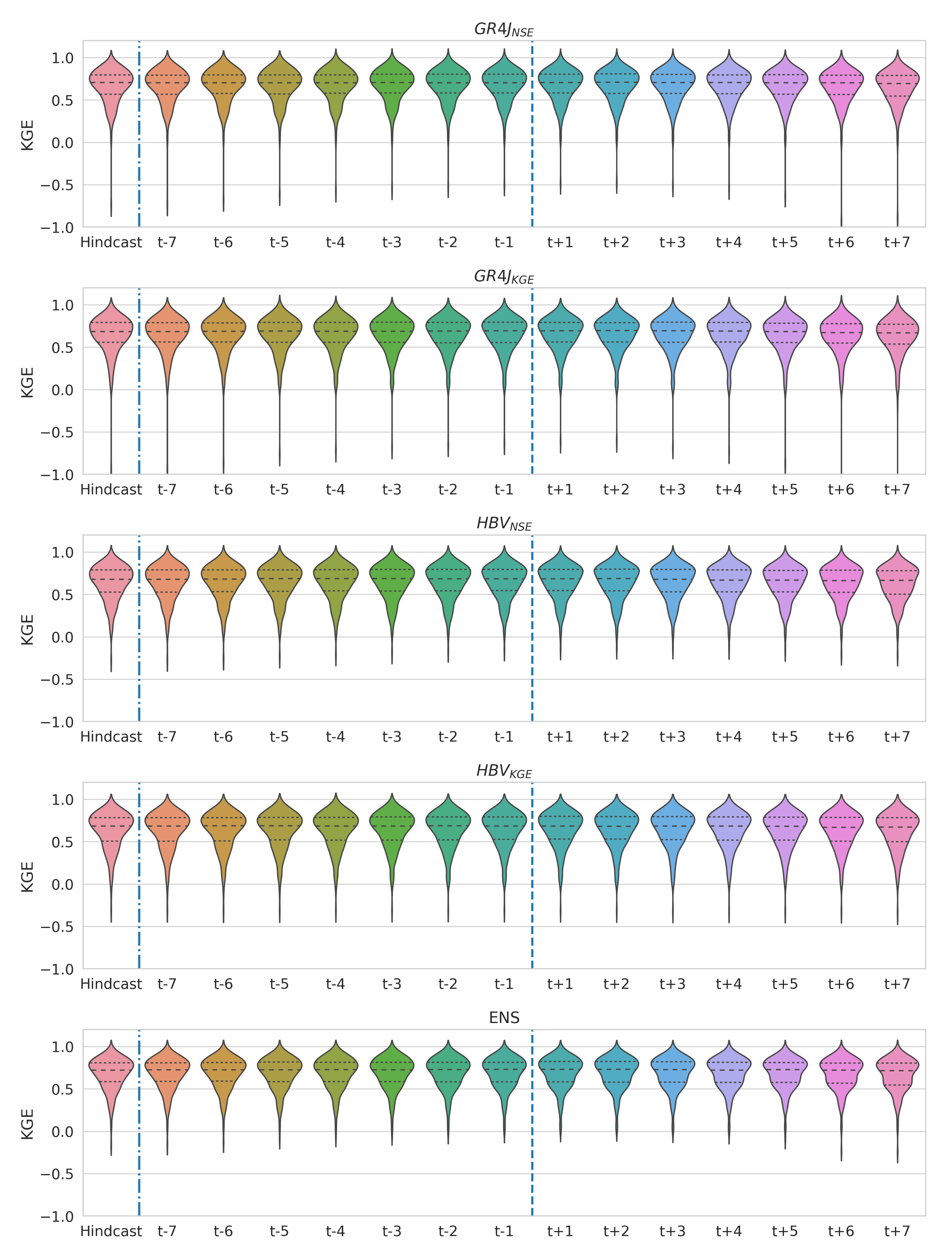
  • While the OpenForecast system utilizes different sources of meteorological data for different modeling phases (Figure 1 and Figure 2), there are no distinct gaps in model performance between them (Figure 6). The additional exciting insight obtained: simpler models have comparable or even higher reliability on the evaluation period than more complex models even while demonstrating similar results on the calibration period.
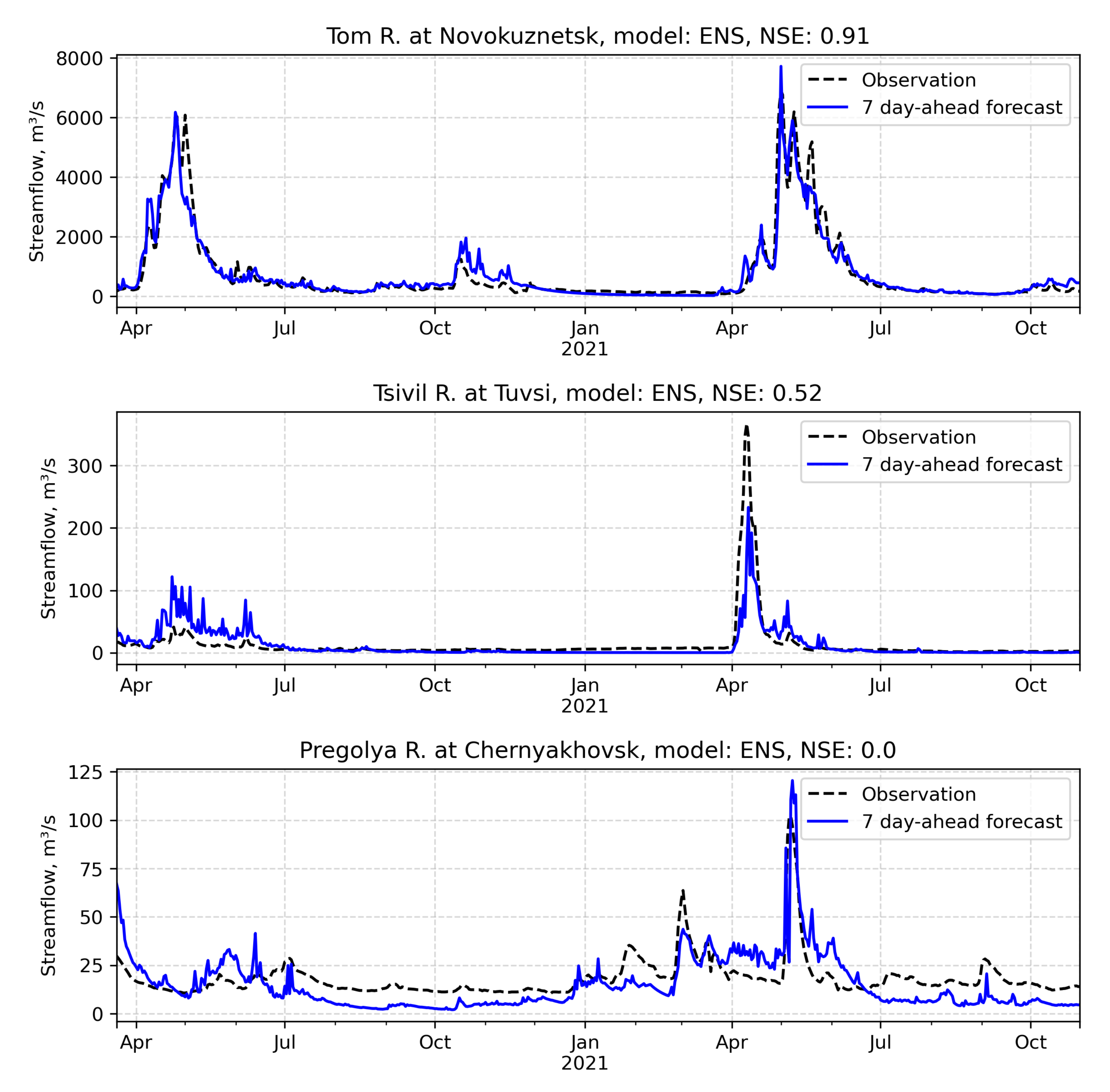
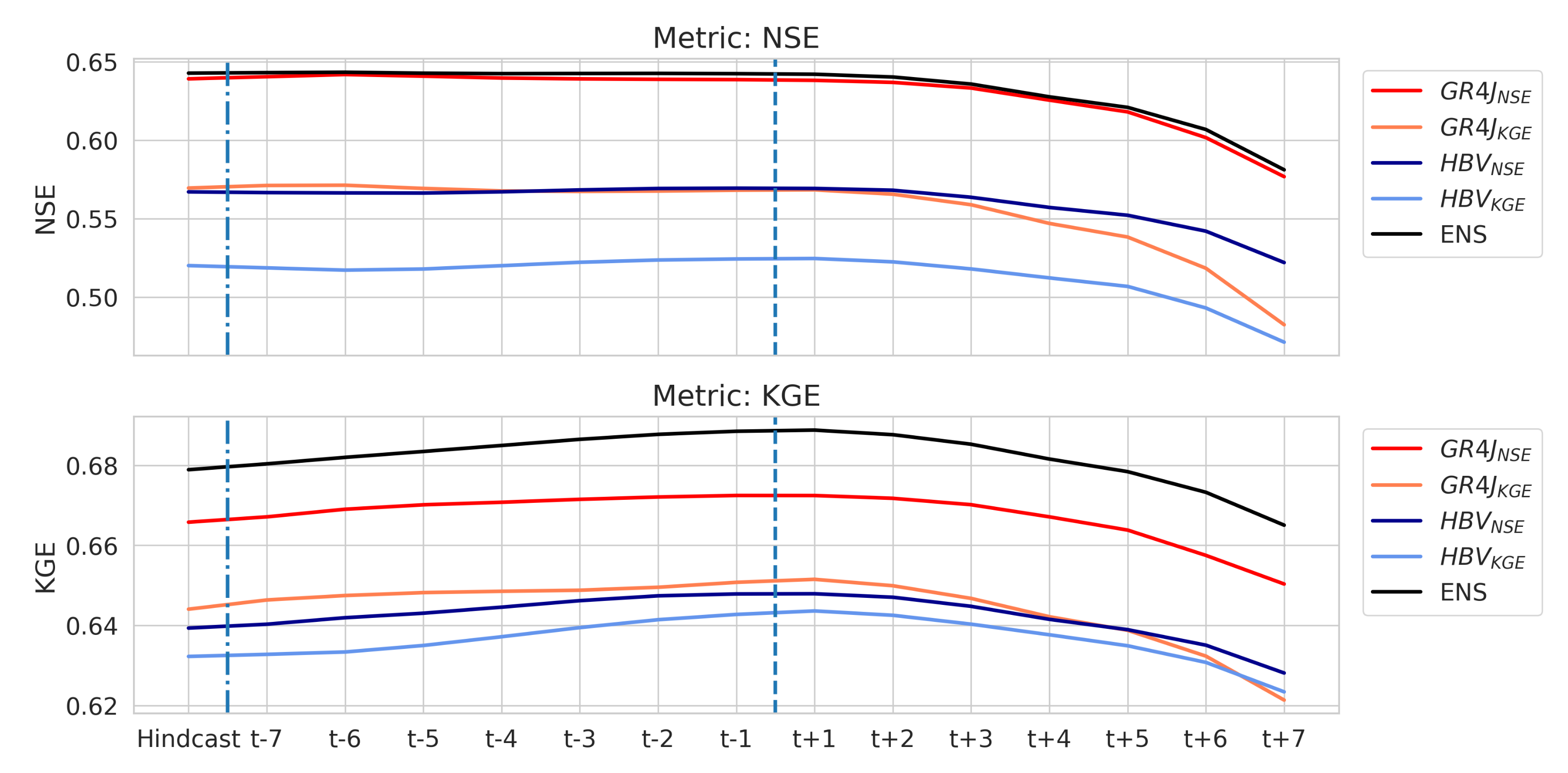
  • The ensemble mean of individual model forecast realizations outperforms each model in terms of NSE and KGE for all considered evaluation periods and lead times (Figure 8). That underlines that the communication of ensemble mean with the end-users is the best dissemination strategy so far.
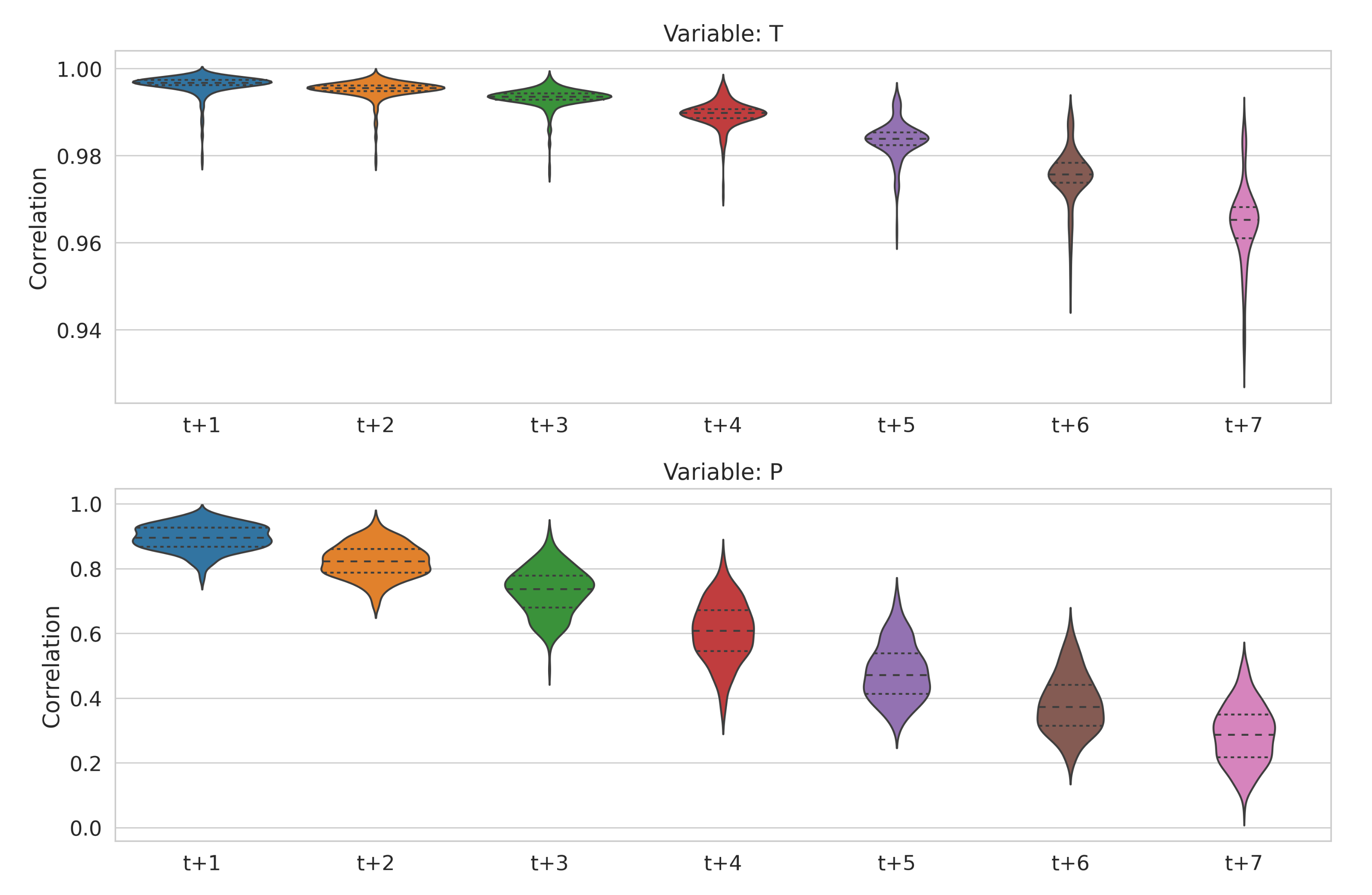
  • Despite the recent advances in numerical weather prediction, the skill of one-week-ahead precipitation forecasting remains the main (unsolved) problem in the forecasting chain (Figure 9). However, due to the comparatively high inertia of runoff formation processes on a watershed, uncertainties of precipitation forecast do not entirely transfer to the runoff predictions.
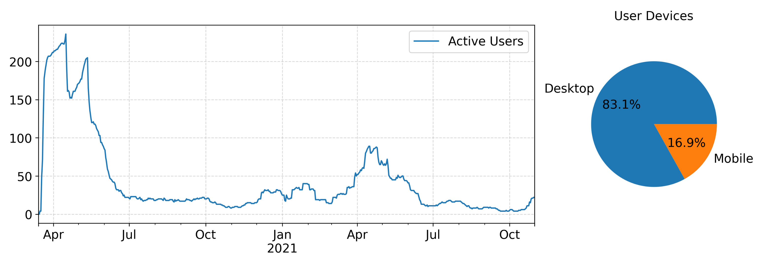
  • User engagement in accessing runoff forecasting systems is low and mostly limited to flood-rich periods (March–July) (Figure 10). That makes costs of idle systems high and requires new, mobile-first approaches to deliver runoff forecasts to the general public efficiently.
In summary, OpenForecast could be considered as a successful national-scale forecasting service that delivers timely and reliable runoff predictions for hundreds of gauges across Russia. In further studies, we will continue to capitalize on the increasing diversity of issued runoff ensembles by increasing the number of utilized hydrological models and sources of meteorological forecast data. In addition, we admit an ample potential of deep learning techniques to be utilized on different stages of the forecasting chain to increase its efficiency.

Author Contributions

Conceptualization, G.A.; methodology, G.A. and D.A.; software, G.A. and D.A.; formal analysis, G.A.; investigation, G.A.; resources, G.A.; data curation, G.A.; writing—original draft preparation, G.A.; writing—review and editing, G.A. and D.A.; visualization, G.A. and D.A.; funding acquisition, G.A. All authors have read and agreed to the published version of the manuscript.

Funding

The reported study was funded by the Russian Foundation for Basic Research (RFBR) according to the research projects Nos. 19-05-00087 and 19-35-60005.

Institutional Review Board Statement

Not applicable.

Informed Consent Statement

Not applicable.

Data Availability Statement

Data sets supporting reported results are published in an open-access research repository at https://doi.org/10.5281/zenodo.5801141 (accessed on 23 December 2021).

Conflicts of Interest

The authors declare no conflict of interest.

Appendix A

Figure A1. Differences between individual hydrological model performances in terms of KGE for calibration and hindcast (evaluation) periods. Violin plots represent the distribution of estimated values within the full range of variation. Dashed lines show the quantiles of 25, 50, and 75%, respectively.
Geosciences 12 00067 g0a1
Figure A2. Differences between performances of individual hydrological models and their ensemble mean for the hindcast, pre-operational hindcast, and forecast modeling phases in terms of KGE. Violin plots represent the distribution of estimated values within the full range of variation. Dashed lines show the quantiles of 25, 50, and 75%, respectively.
Geosciences 12 00067 g0a2

References

  1. CRED. Natural Disasters 2019. 2020. Available online: https://emdat.be/sites/default/files/adsr_2019.pdf (accessed on 10 December 2021).
  2. CRED. Cred Crunch 62 -2020 Annual Report. 2021. Available online: https://cred.be/sites/default/files/CredCrunch64.pdf (accessed on 10 December 2021).
  3. Ward, P.J.; Blauhut, V.; Bloemendaal, N.; Daniell, J.E.; de Ruiter, M.C.; Duncan, M.J.; Emberson, R.; Jenkins, S.F.; Kirschbaum, D.; Kunz, M.; et al. Review article: Natural hazard risk assessments at the global scale. Nat. Hazards Earth Syst. Sci. 2020, 20, 1069–1096. [Google Scholar] [CrossRef] [Green Version]
  4. Jonkman, S.N. Global perspectives on loss of human life caused by floods. Nat. Hazards 2005, 34, 151–175. [Google Scholar] [CrossRef]
  5. Blöschl, G.; Hall, J.; Viglione, A.; Perdigão, R.A.; Parajka, J.; Merz, B.; Lun, D.; Arheimer, B.; Aronica, G.T.; Bilibashi, A.; et al. Changing climate both increases and decreases European river floods. Nature 2019, 573, 108–111. [Google Scholar] [CrossRef] [PubMed]
  6. Blöschl, G.; Kiss, A.; Viglione, A.; Barriendos, M.; Böhm, O.; Brázdil, R.; Coeur, D.; Demarée, G.; Llasat, M.C.; Macdonald, N.; et al. Current European flood-rich period exceptional compared with past 500 years. Nature 2020, 583, 560–566. [Google Scholar] [CrossRef]
  7. IPCC. Global Warming of 1.5 °C: An IPCC Special Report on the Impacts of Global Warming of 1.5 °C above Pre-Industrial Levels and Related Global Greenhouse Gas Emission Pathways, in the Context of Strengthening the Global Response to the Threat of Climate Change, Sustainable Development, and Efforts to Eradicate Poverty; Intergovernmental Panel on Climate Change: Geneva, Switzerland, 2018. [Google Scholar]
  8. Sivapalan, M.; Savenije, H.H.; Blöschl, G. Socio-hydrology: A new science of people and water. Hydrol. Process. 2012, 26, 1270–1276. [Google Scholar] [CrossRef]
  9. Baldassarre, G.D.; Viglione, A.; Carr, G.; Kuil, L.; Salinas, J.; Blöschl, G. Socio-hydrology: Conceptualising human-flood interactions. Hydrol. Earth Syst. Sci. 2013, 17, 3295–3303. [Google Scholar] [CrossRef] [Green Version]
  10. Frolova, N.; Kireeva, M.; Magrickiy, D.; Bologov, M.; Kopylov, V.; Hall, J.; Semenov, V.; Kosolapov, A.; Dorozhkin, E.; Korobkina, E.; et al. Hydrological hazards in Russia: Origin, classification, changes and risk assessment. Nat. Hazards 2017, 88, 103–131. [Google Scholar] [CrossRef]
  11. Pappenberger, F.; Cloke, H.L.; Parker, D.J.; Wetterhall, F.; Richardson, D.S.; Thielen, J. The monetary benefit of early flood warnings in Europe. Environ. Sci. Policy 2015, 51, 278–291. [Google Scholar] [CrossRef]
  12. Pagano, T.C.; Wood, A.W.; Ramos, M.H.; Cloke, H.L.; Pappenberger, F.; Clark, M.P.; Cranston, M.; Kavetski, D.; Mathevet, T.; Sorooshian, S.; et al. Challenges of Operational River Forecasting. J. Hydrometeorol. 2014, 15, 1692–1707. [Google Scholar] [CrossRef] [Green Version]
  13. Alfieri, L.; Burek, P.; Dutra, E.; Krzeminski, B.; Muraro, D.; Thielen, J.; Pappenberger, F. GloFAS: Global ensemble streamflow forecasting and flood early warning. Hydrol. Earth Syst. Sci. 2013, 17, 1161–1175. [Google Scholar] [CrossRef] [Green Version]
  14. Emerton, R.; Zsoter, E.; Arnal, L.; Cloke, H.L.; Muraro, D.; Prudhomme, C.; Stephens, E.M.; Salamon, P.; Pappenberger, F. Developing a global operational seasonal hydro-meteorological forecasting system: GloFAS-Seasonal v1.0. Geosci. Model Dev. 2018, 11, 3327–3346. [Google Scholar] [CrossRef] [Green Version]
  15. Harrigan, S.; Zoster, E.; Cloke, H.; Salamon, P.; Prudhomme, C. Daily ensemble river discharge reforecasts and real-time forecasts from the operational Global Flood Awareness System. Hydrol. Earth Syst. Sci. Discuss. 2020, 2020, 1–22. [Google Scholar] [CrossRef]
  16. Thielen, J.; Bartholmes, J.; Ramos, M.H.; de Roo, A. The European Flood Alert System–Part 1: Concept and development. Hydrol. Earth Syst. Sci. 2009, 13, 125–140. [Google Scholar] [CrossRef] [Green Version]
  17. Bartholmes, J.C.; Thielen, J.; Ramos, M.H.; Gentilini, S. The european flood alert system EFAS–Part 2: Statistical skill assessment of probabilistic and deterministic operational forecasts. Hydrol. Earth Syst. Sci. 2009, 13, 141–153. [Google Scholar] [CrossRef] [Green Version]
  18. Robertson, D.E.; Shrestha, D.L.; Wang, Q.J. Post-processing rainfall forecasts from numerical weather prediction models for short-term streamflow forecasting. Hydrol. Earth Syst. Sci. 2013, 17, 3587–3603. [Google Scholar] [CrossRef] [Green Version]
  19. Massazza, G.; Tarchiani, V.; Andersson, J.C.M.; Ali, A.; Ibrahim, M.H.; Pezzoli, A.; de Filippis, T.; Rocchi, L.; Minoungou, B.; Gustafsson, D.; et al. Downscaling Regional Hydrological Forecast for Operational Use in Local Early Warning: HYPE Models in the Sirba River. Water 2020, 12, 3504. [Google Scholar] [CrossRef]
  20. Ayzel, G. OpenForecast v2: Development and Benchmarking of the First National-Scale Operational Runoff Forecasting System in Russia. Hydrology 2021, 8, 3. [Google Scholar] [CrossRef]
  21. McMillan, H.K.; Booker, D.J.; Cattoën, C. Validation of a national hydrological model. J. Hydrol. 2016, 541, 800–815. [Google Scholar] [CrossRef]
  22. Cohen, S.; Praskievicz, S.; Maidment, D.R. Featured Collection Introduction: National Water Model. JAWRA J. Am. Water Resour. Assoc. 2018, 54, 767–769. [Google Scholar] [CrossRef] [Green Version]
  23. Ehret, U. Evaluation of operational weather forecasts: Applicability for flood forecasting in alpine Bavaria. Meteorol. Z. 2011, 20, 373–381. [Google Scholar] [CrossRef]
  24. Ayzel, G.; Varentsova, N.; Erina, O.; Sokolov, D.; Kurochkina, L.; Moreydo, V. OpenForecast: The First Open-Source Operational Runoff Forecasting System in Russia. Water 2019, 11, 1546. [Google Scholar] [CrossRef] [Green Version]
  25. Bugaets, A.; Gartsman, B.; Gelfan, A.; Motovilov, Y.; Sokolov, O.; Gonchukov, L.; Kalugin, A.; Moreido, V.; Suchilina, Z.; Fingert, E. The Integrated System of Hydrological Forecasting in the Ussuri River Basin Based on the ECOMAG Model. Geosciences 2018, 8, 5. [Google Scholar] [CrossRef] [Green Version]
  26. Cloke, H.; Pappenberger, F. Ensemble flood forecasting: A review. J. Hydrol. 2009, 375, 613–626. [Google Scholar] [CrossRef]
  27. Emerton, R.E.; Stephens, E.M.; Pappenberger, F.; Pagano, T.C.; Weerts, A.H.; Wood, A.W.; Salamon, P.; Brown, J.D.; Hjerdt, N.; Donnelly, C.; et al. Continental and global scale flood forecasting systems. Wiley Interdiscip. Rev. Water 2016, 3, 391–418. [Google Scholar] [CrossRef] [Green Version]
  28. Wu, W.; Emerton, R.; Duan, Q.; Wood, A.W.; Wetterhall, F.; Robertson, D.E. Ensemble flood forecasting: Current status and future opportunities. WIREs Water 2020, 7, e1432. [Google Scholar] [CrossRef]
  29. Robson, A.; Moore, R.; Wells, S.; Rudd, A.; Cole, S.; Mattingley, P. Understanding the Performance of Flood Forecasting Models; Technical Report SC130006; Environment Agency: Bristol, UK, 2017. [Google Scholar]
  30. Hersbach, H.; Bell, B.; Berrisford, P.; Hirahara, S.; Horányi, A.; Muñoz-Sabater, J.; Nicolas, J.; Peubey, C.; Radu, R.; Schepers, D.; et al. The ERA5 global reanalysis. Q. J. R. Meteorol. Soc. 2020, 146, 1999–2049. [Google Scholar] [CrossRef]
  31. Reinert, D.; Prill, F.; Frank, H.; Denhard, M.; Baldauf, M.; Schraff, C.; Gebhardt, C.; Marsigli, C.; Zängl, G. DWD Database Reference for the Global and Regional ICON and ICON-EPS Forecasting System; Technical Report Version 2.1.1; Deutscher Wetterdienst (DWD): Offenbach, Germany, 2020. [Google Scholar] [CrossRef]
  32. Oudin, L.; Hervieu, F.; Michel, C.; Perrin, C.; Andréassian, V.; Anctil, F.; Loumagne, C. Which potential evapotranspiration input for a lumped rainfall–runoff model?: Part 2—Towards a simple and efficient potential evapotranspiration model for rainfall–runoff modelling. J. Hydrol. 2005, 303, 290–306. [Google Scholar] [CrossRef]
  33. Lindström, G. A simple automatic calibration routine for the HBV model. Hydrol. Res. 1997, 28, 153–168. [Google Scholar] [CrossRef] [Green Version]
  34. Perrin, C.; Michel, C.; Andréassian, V. Improvement of a parsimonious model for streamflow simulation. J. Hydrol. 2003, 279, 275–289. [Google Scholar] [CrossRef]
  35. Valéry, A.; Andréassian, V.; Perrin, C. ‘As simple as possible but not simpler’: What is useful in a temperature-based snow-accounting routine? Part 1–Comparison of six snow accounting routines on 380 catchments. J. Hydrol. 2014, 517, 1166–1175. [Google Scholar] [CrossRef]
  36. Valéry, A.; Andréassian, V.; Perrin, C. ‘As simple as possible but not simpler’: What is useful in a temperature-based snow-accounting routine? Part 2—Sensitivity analysis of the Cemaneige snow accounting routine on 380 catchments. J. Hydrol. 2014, 517, 1176–1187. [Google Scholar] [CrossRef]
  37. Nash, J.E.; Sutcliffe, J.V. River flow forecasting through conceptual models part I—A discussion of principles. J. Hydrol. 1970, 10, 282–290. [Google Scholar] [CrossRef]
  38. Gupta, H.V.; Kling, H.; Yilmaz, K.K.; Martinez, G.F. Decomposition of the mean squared error and NSE performance criteria: Implications for improving hydrological modelling. J. Hydrol. 2009, 377, 80–91. [Google Scholar] [CrossRef] [Green Version]
  39. Troin, M.; Arsenault, R.; Wood, A.W.; Brissette, F.; Martel, J.L. Generating Ensemble Streamflow Forecasts: A Review of Methods and Approaches Over the Past 40 Years. Water Resour. Res. 2021, 57, e2020WR028392. [Google Scholar] [CrossRef]
  40. Knoben, W.J.M.; Freer, J.E.; Woods, R.A. Technical note: Inherent benchmark or not? Comparing Nash–Sutcliffe and Kling–Gupta efficiency scores. Hydrol. Earth Syst. Sci. 2019, 23, 4323–4331. [Google Scholar] [CrossRef] [Green Version]
  41. Demargne, J.; Mullusky, M.; Werner, K.; Adams, T.; Lindsey, S.; Schwein, N.; Marosi, W.; Welles, E. Application of forecast verification science to operational river forecasting in the US National Weather Service. Bull. Am. Meteorol. Soc. 2009, 90, 779–784. [Google Scholar] [CrossRef] [Green Version]
  42. Santos, L.; Thirel, G.; Perrin, C. Technical note: Pitfalls in using log-transformed flows within the KGE criterion. Hydrol. Earth Syst. Sci. 2018, 22, 4583–4591. [Google Scholar] [CrossRef] [Green Version]
  43. Schaefli, B.; Gupta, H.V. Do Nash values have value? Hydrol. Process. 2007, 21, 2075–2080. [Google Scholar] [CrossRef] [Green Version]
  44. Coron, L.; Andréassian, V.; Perrin, C.; Lerat, J.; Vaze, J.; Bourqui, M.; Hendrickx, F. Crash testing hydrological models in contrasted climate conditions: An experiment on 216 Australian catchments. Water Resour. Res. 2012, 48. [Google Scholar] [CrossRef] [Green Version]
  45. Nicolle, P.; Andréassian, V.; Royer-Gaspard, P.; Perrin, C.; Thirel, G.; Coron, L.; Santos, L. Technical note: RAT–a robustness assessment test for calibrated and uncalibrated hydrological models. Hydrol. Earth Syst. Sci. 2021, 25, 5013–5027. [Google Scholar] [CrossRef]
  46. Ayzel, G. Runoff predictions in ungauged Arctic basins using conceptual models forced by reanalysis data. Water Resour. 2018, 45, 1–7. [Google Scholar] [CrossRef]
  47. Ayzel, G.; Heistermann, M. The effect of calibration data length on the performance of a conceptual hydrological model versus LSTM and GRU: A case study for six basins from the CAMELS dataset. Comput. Geosci. 2021, 149, 104708. [Google Scholar] [CrossRef]
  48. Moriasi, D.; Arnold, J.; van Liew, M.; Binger, R.; Harmel, R.; Veith, T. Model evaluation guidelines for systematic quantification of accuracy in watershed simulations. Trans. ASABE 2007, 50, 885–900. [Google Scholar] [CrossRef]
  49. Clark, M.P.; Vogel, R.M.; Lamontagne, J.R.; Mizukami, N.; Knoben, W.J.M.; Tang, G.; Gharari, S.; Freer, J.E.; Whitfield, P.H.; Shook, K.R.; et al. The Abuse of Popular Performance Metrics in Hydrologic Modeling. Water Resour. Res. 2021, 57, e2020WR029001. [Google Scholar] [CrossRef]
  50. Ayzel, G.; Sorokin, A. Development and evaluation of national-scale operational hydrological forecasting services in Russia. In Proceedings of the CEUR Workshop Proceedings, Khabarovsk, Russia, 14–16 September 2021; pp. 135–141. [Google Scholar]
  51. Pappenberger, F.; Stephens, E.; Thielen, J.; Salamon, P.; Demeritt, D.; van Andel, S.J.; Wetterhall, F.; Alfieri, L. Visualizing probabilistic flood forecast information: Expert preferences and perceptions of best practice in uncertainty communication. Hydrol. Process. 2013, 27, 132–146. [Google Scholar] [CrossRef]
  52. Kuncheva, L.I.; Whitaker, C.J. Measures of diversity in classifier ensembles and their relationship with the ensemble accuracy. Mach. Learn. 2003, 51, 181–207. [Google Scholar] [CrossRef]
  53. Zhou, Z.H. Ensemble Methods: Foundations and Algorithms; Chapman and Hall/CRC: Boca Raton, FL, USA, 2019. [Google Scholar]
  54. Zhang, C.; Ma, Y. Ensemble Machine Learning: Methods and Applications; Springer: Berlin/Heidelberg, Germany, 2012. [Google Scholar]
  55. Ganaie, M.A.; Hu, M.; Tanveer, M.; Suganthan, P.N. Ensemble deep learning: A review. arXiv 2021, arXiv:2104.02395. [Google Scholar]
  56. Knoben, W.J.M.; Freer, J.E.; Fowler, K.J.A.; Peel, M.C.; Woods, R.A. Modular Assessment of Rainfall–Runoff Models Toolbox (MARRMoT) v1.2: An open-source, extendable framework providing implementations of 46 conceptual hydrologic models as continuous state-space formulations. Geosci. Model Dev. 2019, 12, 2463–2480. [Google Scholar] [CrossRef] [Green Version]
  57. Craig, J.R.; Brown, G.; Chlumsky, R.; Jenkinson, R.W.; Jost, G.; Lee, K.; Mai, J.; Serrer, M.; Sgro, N.; Shafii, M.; et al. Flexible watershed simulation with the Raven hydrological modelling framework. Environ. Model. Softw. 2020, 129, 104728. [Google Scholar] [CrossRef]
  58. Dal Molin, M.; Kavetski, D.; Fenicia, F. SuperflexPy 1.3.0: An open-source Python framework for building, testing, and improving conceptual hydrological models. Geosci. Model Dev. 2021, 14, 7047–7072. [Google Scholar] [CrossRef]
  59. Beven, K. Towards integrated environmental models of everywhere: Uncertainty, data and modelling as a learning process. Hydrol. Earth Syst. Sci. 2007, 11, 460–467. [Google Scholar] [CrossRef]
  60. Beven, K. Facets of uncertainty: Epistemic uncertainty, non-stationarity, likelihood, hypothesis testing, and communication. Hydrol. Sci. J. 2016, 61, 1652–1665. [Google Scholar] [CrossRef] [Green Version]
  61. Bauer, P.; Thorpe, A.; Brunet, G. The quiet revolution of numerical weather prediction. Nature 2015, 525, 47–55. [Google Scholar] [CrossRef] [PubMed]
  62. Schultz, M.G.; Betancourt, C.; Gong, B.; Kleinert, F.; Langguth, M.; Leufen, L.H.; Mozaffari, A.; Stadtler, S. Can deep learning beat numerical weather prediction? Philos. Trans. R. Soc. A Math. Phys. Eng. Sci. 2021, 379, 20200097. [Google Scholar] [CrossRef] [PubMed]
  63. Ravuri, S.; Lenc, K.; Willson, M.; Kangin, D.; Lam, R.; Mirowski, P.; Fitzsimons, M.; Athanassiadou, M.; Kashem, S.; Madge, S.; et al. Skilful precipitation nowcasting using deep generative models of radar. Nature 2021, 597, 672–677. [Google Scholar] [CrossRef]
Figure 1. Illustration of the OpenForecast workflow.
Geosciences 12 00067 g001
Figure 2. Illustration of the temporal sequence of modeling phases and the corresponding input data.
Geosciences 12 00067 g002
Figure 3. The spatial location of OpenForecast gauges (n = 843) and those from the ESIMO database that were selected for the verification procedure (n = 252).
Geosciences 12 00067 g003
Figure 4. Differences between individual hydrological model performances in terms of NSE for calibration and hindcast (evaluation) periods. Violin plots represent the distribution of estimated values within the full range of variation. Dashed lines show the quantiles of 25, 50, and 75%, respectively.
Geosciences 12 00067 g004
Figure 5. Spatial distribution of differences between performances of calibration and hindcast periods for the H B V K G E model.
Geosciences 12 00067 g005
Figure 6. Differences between performances of individual hydrological models and their ensemble mean for the hindcast, pre-operational hindcast, and forecast modeling phases in terms of NSE. Violin plots represent the distribution of estimated values within the full range of variation. Dashed lines show the quantiles of 25, 50, and 75%, respectively.
Geosciences 12 00067 g006
Figure 7. Time series of observed and predicted (7-day ahead ensemble mean) streamflow for gauges with high (top panel), medium (middle panel), and low (bottom panel) NSE.
Geosciences 12 00067 g007
Figure 8. Mean values of individual model efficiencies and their ensemble mean for the evaluation period (hindcast, pre-operational hindcast, and forecast) in terms of NSE (top panel) and KGE (bottom panel) metrics.
Geosciences 12 00067 g008
Figure 9. Evaluation-period correlation coefficients between ERA5 reanalysis and ICON forecast data with increasing lead times for air temperature (P, top panel) and precipitation (T, bottom panel).
Geosciences 12 00067 g009
Figure 10. OpenForecast daily users and the distribution of their device types.
Geosciences 12 00067 g010
Table 1. Description and calibration ranges for GR4J model parameters (based on Ayzel [20]).
ParametersDescriptionCalibration Range
X1Production store capacity (mm)0–3000
X2Intercatchment exchange coefficient (mm/day)−10–10
X3Routing store capacity (mm)0–1000
X4Time constant of unit hydrograph (day)0–20
X5Dimensionless weighting coefficient of the snowpack thermal state0–1
X6Day-degree rate of melting (mm/(day*°C))0–10
Table 2. Description and calibration ranges for HBV model parameters (based on Ayzel [20]).
ParametersDescriptionCalibration Range
TTThreshold temperature when precipitation is simulated as snowfall (°C) 2.5 –2.5
SFCFSnowfall gauge undercatch correction factor1–1.5
CWHWater holding capacity of snow0–0.2
CFMAXMelt rate of the snowpack (mm/(day*°C))0.5–5
CFRRefreezing coefficient0–0.1
FCMaximum water storage in the unsaturated-zone store (mm)50–700
LPSoil moisture value above which actual evaporation reaches potential evaporation0.3–1
BETAShape coefficient of recharge function1–6
UZLThreshold parameter for extra outflow from upper zone (mm)0–100
PERCMaximum percolation to lower zone (mm/day)0–6
K0Additional recession coefficient of upper groundwater store (1/day)0.05–0.99
K1Recession coefficient of upper groundwater store (1/day)0.01–0.8
K2Recession coefficient of lower groundwater store (1/day)0.001–0.15
MAXBASLength of equilateral triangular weighting function (day)1–3
Publisher’s Note: MDPI stays neutral with regard to jurisdictional claims in published maps and institutional affiliations.

