Abstract
For the Altai Mountains’ region, especially the arid southeastern part of the Russian Altai, the data on glacier fluctuations in the Pleistocene and Holocene are still inconsistent. The study area was the Kargy River’s valley (2288–2387 m a.s.l.), a location that is not currently affected by glaciation and the glacial history of which is poorly studied. Field observations and geomorphological mapping were used to reveal the configuration of Pleistocene moraines. The relative dating method was applied to define the degree of weathering as an indicator of age. Three moraine groups of different ages (presumably MIS 6, MIS 4, and MIS 2) were identified based on a detailed investigation of their morphological features and the use of relative dating approaches. The latter were primarily based on weathering patterns. Data on the rock mineralogy, porosity, and specificity of biological colonization as an agent of weathering were obtained for the moraine debris. The studied moraines were composed of fine-grained schist, in which the specific surface area and fractality (self-similarity) were more developed in the older moraine. The growth of biota (crustose lichen and micromycetes) colonizing the rock surface led to rock disintegration and the accumulation of autochthonous fragments on the rock surface. Despite the fact that the initial stage(s) of moraine weathering affected by biota was fixed, the correlation trends of biota activity and moraine ages were not determined.
1. Introduction
The study of the Quaternary history of mountain regions around the world is impossible without the use of different numeric techniques to determine the age of sediments [1]; however, the precision and accuracy of such techniques differ and are affected by the climatic conditions of the region studied (e.g., aridity and negative annual temperatures). For the Altai Mountains, the number, timing, and extent of Pleistocene glaciations are still a matter of discussion. The number of glaciations distinguished in the Altai region has differed among studies, with either four (one in the Early Pleistocene, two in the Middle Pleistocene, and one in the Late Pleistocene) [2,3], three (one in the Early Pleistocene, one in the Middle Pleistocene, and one in the Late Pleistocene [4,5,6]; or one in the Middle Pleistocene and two in the Late Pleistocene [7]), or two (in the Middle Pleistocene and in the Late Pleistocene) [8,9,10,11,12,13,14] glaciations being described. Until now, glaciation during the Late Pleistocene has been the best documented; however, some researchers have distinguished a single glaciation [5,6,12,14,15], while some have identified two glaciations [2,3,7,16,17,18].
In addition, different time intervals have been proposed for the maximum advancement of glaciers in the Late Pleistocene by different researchers: MIS 5 [19,20], MIS 4 [21,22], MIS 3 [23], or MIS 2 [24,25,26].
Thus, there are different points of view on the chronology and scale of glacial events. This is largely due to the use of different methods for sediment dating, the results of which are often inconsistent. Each method has serious limitations in its application. For example, Agatova et. al. [27] studied the applicability of the TL method for the dating of glacial sediments in Chagan-Uzun. It was found out that the dating results of the same sample, performed in different laboratories, were very different, and both had poor agreement with the stratigraphic position of the samples in the section. The main conclusion from independent dating is that the thermoluminescence method works well for loesses, is used for proluvial, and can be applied to lacustrine deposits. However, it is not suitable for dating moraine deposits.
The radiocarbon dating method is limited by time, thus making it mostly inappropriate for the sediments older than MIS 3. Another problem that is quite common for tectonically active mountain areas is the contamination of dated substances with extraneous carbon. For example, this happens in the western and northwestern parts of the Chuya depression, where the organic-rich Middle and Upper Carboniferous, Lower Jurassic, Paleogene, and Neogene deposits are sources of such contamination [28,29]. Another problem is that, in arid areas, glacial deposits are low in organic matter and thus can rarely be used.
Nowadays, surface exposure methods [30] are widely used for the dating of glacial deposits. However, the use of these methods is fraught with problems, in some cases leading to materials being dated as older than they actually are. For others, “rejuvenation” of the dating can occur [31]. Exposure ages that are “too old” appear as a result of pre-exposure to a boulder, either in the bedrock before it falls onto the glacier or if it is reworked from older deposits. Ages that are “too young” result from weathering, instability, and erosion of the moraine surface or shielding by snow cover, soil, vegetation, or lake water and ice (which could be true for the Chuya depression, for example). Destruction of the upper layer of boulders, leading to underestimation of their age, may also be associated with the activity of biota, in particular, lichens. This assumption is based on the results of our current study. For Southeastern Altai, which is a permafrost region, another factor could cause younger ages—the upfreezing of boulders out of a moraine. As a result, the scatter among nuclide measurements from single moraines is often larger than the analytical uncertainty of the method [32,33,34]. Moreover, 10Be-dating, which is the most widely used techniques among the surface-exposure dating methods, requires the presence of a sufficient amount of quartz in the boulders being dated.
Relative dating methods are becoming important for determining the age of glacial deposits. In particular, quantitative relative dating methods are used, wherein the weathering of boulders and soils and degradation of the moraine landform are used as measures of relative moraine age. A quantitative approach to relative dating has also been used since at least the mid-20th century. Characteristics of fresh and weathered granitic clasts were given by [35], and several research studies have used the ratio of fresh-to-weathered granitic stones for this purpose [36,37,38,39].
However, in many cases, the use of granite-weathering ratios gives no result, because “the variety of granitic rock types and their range in relative frequency in drifts related to different valley systems would not permit correlation from valley to valley by this method” [40]. Nevertheless, it was revealed that the decrease in the abundance of surface boulders with age, the slope angle, the loess mantle thickness, and the soil development (the depth to which the underlying gravel has been oxidized) of terraces correlated with the moraines can be used as indicators for relative dating [40]. Devyatkin and Murzaeva developed the method used by Porter and included the several parameters, such as the relative number of shear-strained boulders and the degree of embedment into finely grained material, for the relative dating of moraines in the Mongolian Altai (upper Kobdo depression and Ikh-Turgen eastern slopes) [41]. This method allowed them to distinguish two moraine generations: slightly undulating ancient plains that were poorly developed due to erosion and young hilly depression plains with distinct arcs of several stadial and lateral moraines of different heights and abundant small lakes not deflated by erosion, as well as relic basins and large lakes. It was noted [41] that this method makes it possible to determine their relative ages. However, this principle could be the leading one for the correlation and synchronization of different moraine horizons across the entire Altai–Sayan region, the Mongolian Altai, and Khangai areas [41]. The differences in the morphology of moraines, of course, indicate a significant time interval between their formation, which may well correspond to the interglacial rank.
In the 1980s, the clast-sound velocity (CSV or P-wave velocity measurements) technique [42,43] was developed as an independent relative dating method with which to compare the results of the morphometric analysis. Another approach to measuring the grade of weathering of rocks is the Schmidt-hammer method, which can be used to measure the rebound value (R) and determine the relative surface hardness, providing information on the time of surface exposure and the degree of weathering [44].
This method has been successfully applied for the relative age dating of moraines [45,46,47]. A strong coefficient of determination was found between the Schmidt-hammer rebound number and the P-wave velocity of the tested different rocks [48]. Recently, the pebble count procedure [49] was presented as an additional relative dating technique that could be used to establish relative age relationships among moraines of the same locale [50]. The thickness of the weathering rind, a reddish outer-crust layer around individual rock components, is also used as a possible age marker for moraines and rock glaciers. The reddish rings are a result of the ready oxidation of released Fe affected by chemical weathering [51]. The intensity of chemical weathering is limited by the moisture availability [52] and depends on rock microstructural properties [53]. Rock weathering is also correlated with the pore size distribution [54] and rock fractality [55]. The use of weathering rates from rinds on several rock types for relative to absolute age dating of Quaternary deposits has been discussed [56,57,58,59,60]. In addition, biota (e.g., lichens) can influence to the occurrence of oxidation microzones under the thallus and in the pores penetrated by hyphae [61].
There has been no research on the relative dating of moraines from the arid part of Altai and the neighboring areas with similar geomorphological and climatic features, except for [41,62] and our recent article, which was dedicated to the paleoglaciation of the Mongun-Taiga massif [63]. The present research aimed to apply the relative dating method to define the Pleistocene moraine chronology and configuration based on the Kargy River’s valley located in arid Altai. The relative dating methods used are primarily based on weathering patterns; therefore, data on the rock mineralogy, porosity, and specificity of biological colonization as an agent of weathering were obtained for the moraines.
2. Study area
2.1. Geographical Features
The study area, in which the relative chronology and configuration of Pleistocene moraines were determined, was the Kargy River’s valley in the upper reaches of the river. This area is in the northeastern part of the Dzhulukulskaya depression and the upper part of the Karginskaya depression, which is situated above the present-day tree-line level. The Kargy River flows from the southern slope of the Shapshalsky ridge in the southeastern part of the Altai Mountains (Russia) into lake Ureg-Nur (inland drainless basin of Mongolia) (Figure 1). The river and its valley are adjacent to the divide between the Arctic ocean basins (Ob River and Yenisei River basins).
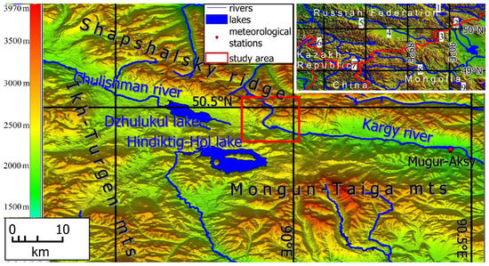
Figure 1.
Location of the study area. Inset: 1—Dzhulukulskaya depression, 2—Mongun-Taiga, 3—Ikh-Turgen, 4—Chuya depression, 5—Kuray depression, 6—Uimon Basin, 7—Kanas valley, 8—Kobdo depression, and 9—Tsambagarav. Elevation is given on the basis of semitransparent digital elevation model SRTM [64].
The height of the watershed along the periphery of the upper course of the Kargy is generally 3100–3300 m, with the highest point (Mount Kat-Taiga) having a height of 3459.4 m.
The upper reaches of the Kargy River (Figure 2) can be divided into several sections. The valley here is narrow (from 200 to 500 m) and rather steep. Initially, it has trough characteristics with a steep (75 m/km on average) bottom and is located at an altitude of 2800 to 2300 m and is directed toward the southwest. The next section, which is about 2.5 km long, is directed toward the southeast. Here, the river cuts through several moraine complexes, and the valley becomes flatter (45 m/km). Further downstream, the river channel takes an east–southeast direction. This section is about 6.6 km long and has a bottom elevation of 2200 to 2100 m. The width of the valley reaches about 4 km.
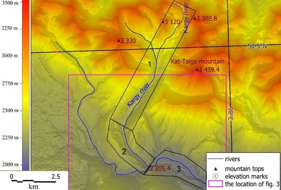
Figure 2.
The upper reaches of the Kargy River. Elevation is given on the basis of semitransparent digital elevation model SRTM [64]. The sections of the valley described in the text are shown in numbers.
Our work was carried out in the elevation range of 2288–2387 m a.s.l.
The relief in the Kargy River’s valley is closely connected with active faults. The river flows along the Dzhulukulskaya, Karginskaya, and Ureg-Nurskaya intermountain depressions (Figure 1), which smoothly replace each other and represent the tectonic Karginskaya depression (1800–2200 m) [7,15,65]. This depression was formed during the Permian–Triassic period (298–252 million years ago) [66] and is in a zone of deep faults: Shapshalsky (Karginskaya) (Figure 2) and Mugur-Aksinsky faults [67]. The Shapshalsky fault is located at the border of the Karginskaya depression with the Shapshalsky ridge. In its upper reaches, Kargy flows along the southern slope of the Shapshalsky ridge, which is composed of rocks from the upper section of the Cambrian and lower section of the Ordovician systems. The rocks are widespread on both sides of the valley and include sandstones, siltstones, schist, and gravelstones; the moraines are mostly composed of the material originating from them. At the foot of the Shapshalsky ridge, along the fault line, the Cambrian and Ordovician rocks are replaced by Jurassic rocks, represented by conglomerates, gravelstones, sandstones, schist, and brown coals. In the lowest section of the upper part of the Kargy River’s valley (No. 3, Figure 2), Miocene deposits are presented by light-gray clays, aleurolites, denes, gravel rocks, and gur coals.
Pre-Quaternary rocks are overlaid by Upper Quaternary [68] or Middle Quaternary [69] glacial deposits (moraines), represented by boulders, gravel, and sands. The outer edge of the moraine, which is a system of arcuate curved hills, is somewhat blurred. The flat depressions between the hills are composed of fluvioglacial pebbles, which occur in erosional hollows that cut through the edge of the moraine. In sections of the valley that are free from moraine, located several kilometers downstream of the river, pebbles form an inclined surface of a fluvioglacial cone, which turns into a 35–37 m high terrace that stretches down the river valley. This terrace has a number of lower terrace-like ledges. Down the valley, the terraces turn into one terrace that is about 25–30 m high [16].
The valley, which is not currently affected by glaciation, is characterized by a sharply continental climate with a low amount of precipitation that is less than the potential evapotranspiration; a large temperature range; and a negative average annual temperature. The closest meteorological station, Mugur-Aksy, which is at an elevation of 1830 m a.s.l., is located 38 km to the east of the study area. Based on data from the station, the mean annual precipitation (MAP) is 156 mm with 75% of that presented as water, and the mean annual temperature (MAT) is −2.6 °C. More than 80% of the precipitation falls in the summer, due to local cyclogenesis. In winter, the region is dominated by the Siberian anticyclone, and as a result, the snow thickness is low (average maximum is 7 cm). The annual amplitude of the mean monthly air temperature is 34.3 °C [70]. Taking into account the elevation difference between the study area and the meteorological station, the regional temperature lapse rate (0.69 °C/100 m) and the altitudinal precipitation gradient calculated for the adjacent Mongun-Taiga massif (7 mm/100 m) [70,71] can be used. The extrapolated MAT varies from −8.1 to −9.6 °C, and the MAP varies from 179 to 193 mm.
2.2. Experience with Relative Dating in Eastern Altai
Little is known about past glaciation in the Kargy River’s valley that is estimated to have occurred in the Middle Quaternary [69] or Upper Quaternary [68]. Nevertheless, only 15 km to the south is the Mongun-Taiga mountain range, and the history of glaciation there has been relatively well studied [63,72]. Four groups of moraines have been distinguished there. The youngest group of moraines (at altitudes over 2600 m a.s.l.) is represented by coarse angular stony material intersected with sand and clay deposits. The moraines are free of vegetation or slightly covered by pioneer vegetation. They have steep fronts and belong to the neoglacial epoch. There are radiocarbon dates that confirm their neoglacial ages, and the age of the most ancient stage among the moraines of this group is within the interval of 5.5–3.6 ka cal BP.
The moraines in the next group are situated within the troughs, reaching 2100–2200 m a.s.l. They are composed of a bluish-gray sandy material and have a large number of rounded boulders that are mostly granite. Their surfaces are covered with herbaceous vegetation and yerniks. The moraines of this group look like arched ramparts, damming up lakes in some valleys. The deglaciation time has been confirmed through 10Be dating as 11.229 ± 1.083 ka [63], so this moraine group is referred to as MIS 2. The warm interval between MIS 2 and the neoglacial period when forest vegetation reached positions that were about 350 higher than the present ones has been proven by several 14C dates in the interval 5.326–10.580 ka cal BP [63]. Large differences in the ages of the moraines were confirmed by the results of relative dating, and all of the parameters, which reflected different degrees of weathering of moraines, showed significant changes [63].
Another moraine group is located at the transition from U-shaped valleys into intermountain depressions, i.e., at altitudes of 1800–2200 m a.s.l. The composition of the moraines is similar to that of the previous group. Their surface is hummocky-like with many small, round thermokarst depressions and lakes, and steppe and tundra vegetation prevail. The 10Be date of deglaciation is 23.633 ± 2.306 ka [63], which could mean that the MIS 2 age is the glacial maximum to which the moraines belong, but this is in poor agreement with the sharply pronounced morphological differences to the moraines of the previous group, as well as the significantly higher degree of weathering, which has been confirmed by some of the relative dating results (increase in the shear-strained boulder percentage; increase in the embedment of the boulders into fine-grained materials). The most probable time period for the advance of this glacier is MIS 4, a suggestion that is indirectly evidenced by the time at which lacustrine transgression (between 76 ± 9 and 90 ± 10 ka BP [73]) occurred in the adjacent Great Lakes Basin (Mongolia) to which the main runoff from the glaciers of the Mongun-Taiga massif was directed. The warm intervals separating the periods of moraine formation in this and previous groups on the territory of the Mongun-Taiga massif have been confirmed by the dating of wood from the highlands (28.759–31.436, 43.688–42.567 ka cal BP, and 57.810 ± (≥1.820) 14C ka BP) [63].
The most ancient moraine has survived erosion fragmentarily and has not been reconstructed in detail. Its surface is strongly leveled and relatively weakly bouldered. No dating investigations have been conducted there. The boulder material of all moraines is mainly granite associated with Devonian intrusions (granitoids (subvolcanic bodies and hypabyssal intrusions)) in the upper part of the glacial basin [74].
At the moment, we have not obtained a sufficient amount of data by using this technique to compare moraines with homogeneous mineralogy compositions. At the same time, the presence of a good sample of observations collected over a very small area with homogenous climatic conditions and morphologically similar moraines makes it possible to check the similarities and differences in the manifestation of weathering processes and the influence of the mineralogy composition on these. In this case, we were prepared for large differences in the relative dating results. It was also interesting to test the hypothesis formed by Devyatkin and Murzaeva about the possibility of synchronizing moraines among the Altai, Sayan, and Khangai regions [41]. Investigation of this hypothesis requires the accumulation of factual material in different valleys, and this work also partly followed this goal. Thus, the variety in the mineralogy of moraines from different valleys—as it is characterized by diverse substrates due to the geological characteristics of the area—makes their comparison difficult.
3. Methods
3.1. Geomorphology Study
At the preliminary stage of the field work, the moraines were delineated in satellite imagery, and the moraines in the Kargy River’s valley were morphologically described. The interpretation of satellite images was performed by using Sentinel-2 imagery (image data 27.08.2019, spatial resolution 10 m) downloaded from the USGS EROS Data Center by [64]. Two variants of band combinations were used: the natural color band combination (B4, B3, and B2) and the B12, B11, and B2 band combination, which is often used for geological studies. We used the standard satellite imagery decoding method, which was developed for the moraine complexes of the Mongun-Taiga massif [72]. To check and refine the results of decoding satellite images, we used the 30 m SRTM 1 Arc-Second Global DEM downloaded from the USGS EROS Data Center [64]. In the process of mapping, we also used field data: ground control points and GPS-tracking results.
3.2. Moraine Relative-Dating Method
The moraine relative dating method used was based on the method proposed by Porter [40] that was developed by Devyatkin and Murzaeva [41] and later supplemented with several additional characteristics (lichen coverage, rock surface hardness (Schmidt hammer rebound value R) [63]. On a moraine polygon with an area of 100 m2, boulders with diameters over 30 cm were counted and analyzed. Then, the following features were delineated: the number of boulders with a diameter over 30 cm (N), the presence of shear-strained boulders (C, %) and flat-topped boulders (F, %), the degree of embedment into fine-grained materials (B, %), lichen coverage (L, %), and rock surface hardness (R) [63]. The rock surface hardness dimension was realized by using an N-type Schmidt hammer [75,76]. This is a portable instrument that was originally developed to test concrete quality in a nondestructive way. It can also measure the rebound value of a boulder [45,75,76]. A spring-loaded bolt on a rock surface yields a rebound (or R-value) that is proportional to the hardness (compressive strength) of the rock surface. All rebound measurements were performed with the hammer held vertically downwards and at a right angle to the horizontal rock faces. According to geomorphology, more weathered surfaces are characterized by low R-values, and less weathered surfaces correspondingly have high R-values [77]. There were 10 to 60 boulders with a diameter over 30 cm on a polygon (on average, about 30 boulders). Each boulder was measured three times with a Schmidt hammer (values were close, so we did not have to exclude outliers). Further, the average R-value was obtained by calculating the arithmetic mean of the three measurements. We did not measure the lichen-covered parts of the boulders or their cracked parts.
3.3. Mineralogy Composition of the Moraine Samples
The mineralogy compositions of the moraines (samples from polygons K1, K2, and K3) were studied in thin sections, by optical microscopy, using a Leica DM LP microscope.
3.4. Specific Surface Area of Moraine Samples and Pore Size Distribution
The specific surface area (the total surface area of a material per unit of mass) and the pore size distribution of the moraines (samples from polygons K1 and K3) were determined with the low-temperature nitrogen adsorption method, using a QuantaChrome Nova 1200e analyzer (Quantachrome Instruments, Boynton Beach, FL, USA). The samples were degassed in a drying chamber at 100 °C for 19 h; then the samples were analyzed by the multipoint Brunauer–Emmett–Teller (BET) method, using 7 points. The pore size distribution was calculated by the Barret–Joyner–Halenda (BJH) method, using the nitrogen desorption isotherm (NOVAWin™—Windows® Based Software for Operation from PC). The method can be used to investigate pores with diameters < 100 nm [78].
3.5. Mesostructure and Fractal Properties of Moraine Samples
The mesostructure (mesostructure data—structural parameters in diapason 2–100 nm) and fractal properties (fractality—self-similarity, which means that the object is exactly or almost the same as a part of itself) of the moraines (samples from the polygons K1 and K2) were investigated by the small angle neutron scattering (SANS) method. The SANS experiment was performed with the “Yellow Submarine” instrument (BBR research reactor in Budapest Neutron Center, Hungary), which operates with near point geometry. Using of neutron wavelength (λ = 0.49 nm, Δλ/λ = 18%) and two sample-to-detector distances (1.6 and 5.6 m) provides the measurements in the momentum transfer range (q) of 6.5 × 10⁻² < q < 4 nm−1 (where: q = 4πλ−1sin(θ/2), θ is the scattering angle) that correspond to the analysis of the rock structure in the range D ≈ 2π/q from 1 to 100 nm. The scattered neutrons were detected by a two-dimensional position-sensitive BF3 gas detector (64 × 64 cells of 1 cm × 1 cm).
The sample powders were placed in 1 mm thick quartz cells. The apparent density ρH of each sample was calculated as the weight of the powder divided by its volume. The raw data were corrected by using the standard procedure [79], taking into account the scattering from the setup equipment and cell. The resulting 2D isotropic spectra were averaged azimuthally and their absolute values were determined by normalizing to the incoherent scattering cross section of water and apparent density ρH for each sample. Data preprocessing was performed by using the BerSANS software [80].
3.6. Identification of Biota on the Rock Surface
The initial analysis of the moraines (samples from polygons K1, K2, and K3), oxidized ring, and lichen distribution on the rock surfaces was carried out by using a Leica M 80 stereomicroscope. Visualization of lichen colonizing the moraine samples was carried out in untreated samples using a Color 3D Laser Microscope (KEYENCE VK-9700 Laser Scanning Microscope, Japan). The morphology of micromycetes and trends in its spatial distribution on the rock surface were studied by using a light microscope (Leica DM 1000), as well as a Scanning Electron Microscope (SEM TM 3000, HITACHI, Japan).
4. Results
4.1. Geomorphology of the Studied Area
In the upper course area, from the northeast to the southwest, the valley of the Kargy River has typical trough characteristics including a U-shaped transverse profile (Figure 3), which indicates its glacial past. The occurrence of glacial processes of erosion and sedimentation is also reflected in the stepped longitudinal profiles of the valley (Figure 3). In the lower reaches of the Kargy River, moraine deposits have typical morphologies and positions for the region and are similar to the glacial deposits of the Mongun-Taiga mountain range. The lowest are the most ancient moraines (group A) which are strongly leveled (Figure 4A) with rare boulders buried in moraine material. These moraines are located in the altitude interval 2185–2500 m a.s.l. in the axial part of the valley, which is located at 2185–2275 m a.s.l. The moraine has a lobed shape (Figure 3). We conclude that the glacier arose from the valley and spread out.
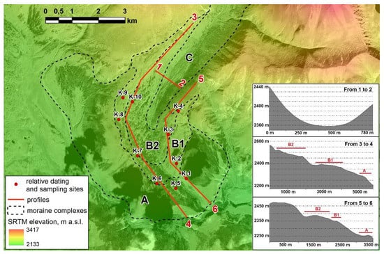
Figure 3.
Spatial distribution of moraines and profiles of the Kargy River’s valley (based on a Sentinel-2 image and semitransparent digital elevation model SRTM [64]). Profiles were created in Global Mapper. A–C represent groups of moraines.
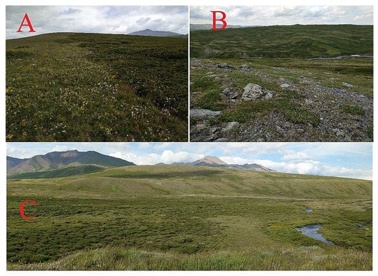
Figure 4.
(A) Moraine from group A, polygon K1, (B) moraine from B2 (polygon K3), and (C) general view of the moraines in the Kargy area from the southwest.
The younger formations (group B) embedded in the above moraine are typically knob-and-kettle moraine formations (Figure 4B). These moraines are clearly subdivided into two stages (B1 and B2). Along the valley, they reach elevations of 2250 and 2290 m a.s.l., respectively. The glacier protruded from the narrow part of the valley, turning from the southwest to the south–southeast direction, but was too short to reach the flatter part, forming only a slight expansion.
The next moraine complex (group C) is outlined by more ancient moraines from group B. These are moraines from a valley glacier. They are situated on the steep slopes of the trough and have been strongly eroded, so there is no clearly visible moraine rampart. The glacier front is located at an altitude of 2325 m a.s.l. On the northwestern side of the trough, the upper limit of the distribution of this moraine is 100 m below the upper edge of the B2 moraines, which probably reflects the difference in glacier thickness during these glacier stages. No younger moraines were found in the valley above the group C moraines. Thus, three groups of moraines of different ages were identified through our detailed investigation of morphological features.
4.2. The Results of Relative Dating
Two of the profiles sampled for moraine relative dating were located along the sides of the Kargy River. Measurements were carried out at 10 polygons (4 polygons on the left side of the valley and 6 polygons on the right side of the valley), where about 280 boulders were described and analyzed (Figure 3 and Figure 4 and Table 2). The choice of polygons used for relative dating was dictated by the distinctness of the moraines, their preservation from the point of view of erosion processes, and the presence of stable areas on the ridges of the moraines. The relative dating methods used are primarily based on weathering patterns. Therefore, we selected moraine samples from three polygons (K3, K2, and K1) to detail several parameters that can be used as indirect dating markers. In our opinion, the study of mineralogy composition and the porosity of moraine samples, as well as investigation of the specificity of biological colonization as an agent of weathering, can provide a better understanding of the significantly different rock ages that show up following weathering.
Two of the studied polygons were located in the areas of group A moraines. They had monotonic surfaces in terms of vegetation cover and boulders occurrence. The largest number of polygons (five) was selected from the surface of complex B1, the length of which was the greatest. Three polygons were identified within complex B2. No horizontal sites could be identified on erosion-resistant surfaces in the territory of complex C; therefore, no work on relative dating was carried out there.
4.3. Mineralogy Composition of Moraines
The moraine samples were composed of fine-grained schist, which is dense, weakly layered, and colored dark gray to black. Schist belongs to the group of regional metamorphism rocks from green schist facies. It is likely that the primary rock was sandstone. The main rock-forming minerals were identified as being quartz (45%), chlorite (pennine) (25%), and sericite (7%). Two generations of quartz were identified: (i) corroded and deformed due to metamorphism within larger (~0.1 mm) grains and (ii) smaller (<0.01 mm) grains. Additionally, actinolite, albite, and rare thin streaks of calcite were found. Calcite is not related to green schist facies and belongs to a younger generation (Figure 5). Iron (hydr)oxides were represented by the separate grains of magnetite and, to a lesser degree, goethite. The presence of thin and light brown films of goethite surrounding the chlorite grains can be attributed to the initial weathering stage of chlorite, which is sensitive to weathering and enriched by iron. The process of chlorite weathering has been enhanced on the rock surfaces, leading to the formation of discontinuous reddish rings.
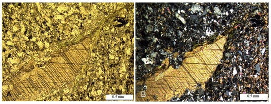
Figure 5.
Thin section of a moraine sample within a large particle of calcite: (A) parallel Nicoli and (B) crossed Nicoli.
4.4. Specific Surface Area of Moraines and Pore Size Distribution
The full nitrogen adsorption–desorption isotherms of the samples (Figure 6A) were found to be characterized by expressed capillary condensation hysteresis and refer to type IV [81], which corresponds to adsorption on mesoporous (diameter 2–100 nm) materials. The shape of the hysteresis loop allowed us to classify it as type H3 [81], a group that presents with non-rigid aggregates of plate-like particles giving rise to slit-shaped pores. The points of joining adsorption and desorption branches of full isotherms are below the values of nitrogen relative pressure P/P0 = 0.3 for all samples, indicating the presence of some micropores (diameter < 2 nm) (Figure 6B). All studied samples were characterized by a lognormal size distribution of pores in the range from 1.5 to 15 nm, with maximum dp values of 2.2 (moraine from polygon K1), 1.7 (moraine from polygon K3, internal (unweathered) part of the boulder), and 1.9 nm (moraine from polygon K3, surface (weathered) part of the boulder) (Figure 6B and Table 1). The texture characteristics of moraine samples obtained through the analysis of full nitrogen adsorption–desorption isotherms, using the BET and BJH models, are summarized in Table 1. There was a predominance of pores with maximum dp ~ 2 nm that tenaciously retain solutes and are associated with the presence of layer silicates [54], and this can be a prerequisite to rock weathering. However, the insignificant differences among the studied samples of moraines of different ages suggest a low rate of rock weathering.
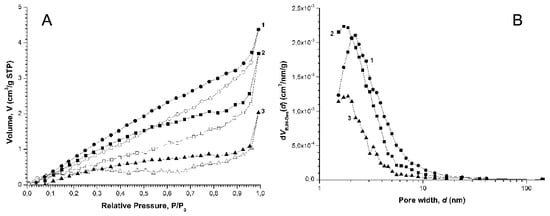
Figure 6.
Full nitrogen adsorption (white)–desorption (black) isotherms (A) and their corresponding pore size distributions dV(D); (B) obtained from the treatment of full nitrogen adsorption–desorption isotherms within the BJH model: (here and in Figure 7) moraine samples from polygons K1 (1) and K3 (2—internal, less weathered part; and 3—surface, more weathered part of the same boulder).

Table 1.
Parameters of the mesostructure of the moraine samples obtained from the analysis of SANS (DS = 6 − n) and low-temperature nitrogen absorption data (SBET, dp, and VP/P0→0.99).
4.5. Mesostructure and Fractal Properties of Moraine Samples
The experimental curves of the differential neutron cross-section dΣ(q)/dΩ versus momentum transfer q for the moraine samples (Figure 7) revealed the same overall shape for all samples, and two characteristic q-ranges were identified. In the range of q < 0.7 nm−1, the dΣ(q)/dΩ satisfies the power law q−n (Figure 7). The values of the exponent n were determined from the slopes of straight-line segments in the experimental dependences dΣ(q)/dΩ plotted on a log–log scale. Their values were found to lie in the range from 3.82 to 3.86 (Table 1). The power law exponent in the range 3 < n ≤ 4 implies that scattering occurs on the fractal surface with dimensions of 2 ≤ DS = 6 − n < 3 [82].
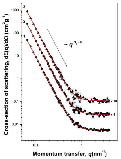
Figure 7.
SANS differential cross-section dΣ(q)/dΩ versus momentum transfer q for the moraine samples (1—from polygon K1; 2 and 3—from polygon K3). Fits of experimental data using equation (1) are shown as solid lines. For the sake of clarity, cross-section values for samples from polygon K3 were multiplied by 5 and 10 (corresponding factors are given next to the curves).
In the region q > 0.7 nm−1, dΣ(q)/dΩ does not depend on q (i.e., it becomes a constant). It is caused then by the incoherent scattering by hydrogen atoms included in the composition of the studied samples in the form of a chemical bound or sorbed water. Therefore, the analysis of the observed scattering and the estimation of the lower bound of self-similarity, r, of the surface fractal were not possible. The absence of a deviation of the dΣ(q)/dΩ curve from the power law (the onset of the Guinier regime) at small values of q means that the upper self-similarity limit ξ of the surface fractal is larger than the maximum size Rmax of the inhomogeneities (pores) that can be detected in the experiment with a given resolution: Rmax = 3.5/qmin ≈ 60 nm. Thus, the observed scattering patterns are typical for scattering from system possessing a disordered porous (solid phase–pore medium) structure with fractal phase boundaries [83,84,85] including natural systems represented by rock fragments from shallow soils [86] and soil aggregates from mature soils [87].
In view of this circumstance, we used the following expression to analyze the scattering from all samples over the entire q range:
where A(DS) is the power-law pre-factor, which depends on the fractal dimensions of the inhomogeneities (pores). The constant Iinc is independent of q and is associated with the incoherent scattering of hydrogen atoms.
Expression (1) was convolved with the instrumental resolution function. The experimental curves of dΣ(q)/dΩ versus q were processed by using the least mean squares method over the entire measured q range. The results of the analysis of the SANS (Figure 7 and Table 1) data revealed that all samples were porous systems with a fractal phase boundary. The sample from polygon K1 was characterized by a more developed fractal surface (DS = 2.18 ± 0.02) than the sample from polygon K3 in both the unweathered (internal part of the boulder) (DS = 2.15 ± 0.02) and more weathered surface parts (oxidized rind) of the boulder (DS = 2.14 ± 0.02). This is clearly consistent with the data of low-temperature nitrogen adsorption. We supposed that the smaller values (approximately two times) obtained for the specific surface area SBET (1.3 m2/g) and the specific volume VP/P0→0.99 (3.9 cm3/g) of the surface part of the sample from polygon K3 compared with its internal part (SBET = 1.3 m2/g and VP/P0→0.99 = 6.7 cm3/g) are probably due to the presence of weathered reddish film, which leads to the closure of some pores. The presence of closed pores in the surface of this sample (from polygon K3) was confirmed by the equality, within the range of experimental error, of the values of the fractal dimension DS = 2.15 ± 0.02 (internal, less weathered part of the boulder) and 2.14 ± 0.02 (surface, more weathered part of the boulder) obtained from the SANS data analysis.
Thus, fractal dimension, DS, which was correlated with a specific surface area, was more pronounced in the sample from polygon K1, indicating its higher weathering level. The differences in the oxidized and unweathered parts from the same sample from polygon K3, which were estimated via the mesostructure, including fractal properties, were insignificant.
4.6. Rock Colonization by Biota
Crustose lichen, which dominated the rock surface, was identified as Dimelaena oreina (Ach.) Norman. Its thallus grows tightly within the substrate, penetrating the rock substrate through microcracks and deepenings (Figure 8A,B). This lichen inhabits open, dry, and sunny places, mostly in the mountains [88]. A clear pattern of moraine colonization by biota from polygon to polygon was not revealed. This was not a disappointment, considering the following two statements: (i) the useful range for lichenometry is 500 years [89], so it cannot be used for moraines of pre-Holocene age; and (ii) in arid conditions, the lichen growth rate differs from that found in humid areas of Altai.
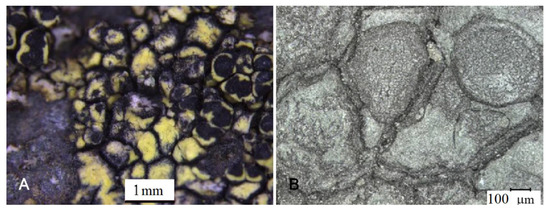
Figure 8.
Dominant crustose lichen Dimelaena oreina on the rock surface: (A) thallus with fruiting bodies (light-microscope data); (B) fruiting bodies (apothecia) embedded into the solid substrate (laser-microscope data).
Micromycetes within specific filamentous structures formed the mycelium nets composing the continuous layers. They are characterized by an irregular distribution and are found mostly on the edges of the rock fragments and the microcavities, whereas most of the rock surface remains uncovered (Figure 9). In microcavities, biota can be better protected against external impacts and can use the organic matter concentrated in the pores, which is a common trend in the northern regions [90]. Penetration of micromycetes inside the rock was shown to occur along the pores, according to a general trend of solid rock colonization [91]. Based on the studied samples, it was revealed that the growth of biota leads to initial biomass accumulation and rock disintegration, along with subsequent autochthonous rock fragment accumulation. The latter remain attached due to the release of extracellular polymeric substances by the biofilms (Figure 10A,B). Thus, the initial stage of rock disintegration is affected by biota.
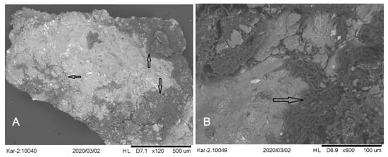
Figure 9.
Rock colonization by micromycetes (arrows) (SEM data): (A) formation of biofilm within the predominance of micromycetes on the edge areas of a stone sample; (B) boundary of the micromycetes’ net and uncovered rock surface.
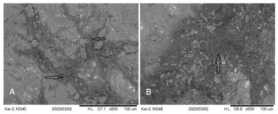
Figure 10.
Locations of micromycetes (arrows) on the disintegrated rock surface: (A) hyphae of a micromycete in fissures and deepening of the rock surface layer; (B) dense interweaving of micromycete hyphae with small fragments of rock on the fungal surface.
5. Discussion
The timing of the of the Upper-Pleistocene glacier advances and the timing of the most extensive glacier advancement in the Altai Mountains are a matter of discussion, mostly due to the differences in approaches and methods used in previous studies. For example, for the Mongolian Altai, it has been reported that major advances took place during MIS4 (74–71 ka, the maximal advance) and MIS2 (25–20 and 18–17 ka) (OSL dating) [21]. However, on the Mongolian side of the Ikh-Turgen mountains (Figure 1), 10Be dating has indicated an age of MIS 3 for the Local Last Glacial Maximum [24].
For the Kanas valley (Chinese Altai), OSL dating revealed that the MIS 3 glaciers were larger than the MIS 2 glaciers [92]. Further work revealed that the largest glacial advance occurred during MIS 6, whereas, during the last glacial cycle, advances occurred during MIS4 (around 73 ka), mid-MIS3 (52–38 ka), and MIS2 (28–16 ka). Here, the local Last Glacial Maximum also is referred to MIS 4 [22]. Subsequently, 14 electron spin resonance (ESR) ages and three optically stimulated luminescence (OSL) ages have been determined in this valley, and together with previous results, these infer that glacial advances took place during MIS 6, 5, 4, 3, and 2. The glacial advance that occurred during MIS 5 is considered the local Last Glacial Maximum, and successive advances (MIS 4-2) were characterized by smaller extents. However, in recent research, the age of the moraine complex, which is supposed to have been formed by several glacier advances (MIS 2, 3, and 3/4) [22,92] was re-evaluated by cosmogenic exposure and single-grain luminescence dating as a MIS 2 complex [26]. The idea that the last glacial cycle in Altai reached its maximum during MIS 2 is being argued by Chinese researchers [23], who stated that the maximal glacial advance in the Xiaokelanhe River (Chinese Altai) occurred in MIS 3 or earlier. Based on an analysis of new and previously published 10Be exposure ages for the Altai Mountains, they suggested that at least three glacier advances occurred during the last glacial cycle in Altai, of which the most extensive occurred before the global LGM during MIS 3 or earlier.
The Russian Altai region has the longest history of moraine dating. The most well-studied site is located in the Chagan-Uzun valley and is closely connected with the history of the ice-dammed Kuray-Chuya paleolake. A comprehensive study using thermoluminescence (TL) dating [4] served as the basis for identifying seven moraines of different ages [93] in the range from 690 to 10 ka BP. Later, the use of a TL technique based on applying naturally saturated etalons [94] showed that the formation of the entire gray-colored strata of the Chagan moraines in this section occurred in the interval from 135 ± 15 to 58 ± 7 ka BP. Later research led the authors of [27] to the conclusion that the use of modern TL technologies for dating moraines is inappropriate.
The appearance of new radiocarbon data in the last 20 years has provided additional information on the ages of interglacial sediments. Two separate units of lake sediments that overlie the glacial deposits with the TL (aged 58 ± 6.7 ka) were dated with 14C 25.3 ± 0.6 ka (MGU IOAN-65, radiocarbon, calibrated with ages 28,741–25,932 BP (1 σ range, 95.4%, OxCal 4.4 [95]) BP, and >45 ka BP (Beta 147107) [96,97]. Later, the older lake unit was additionally sampled and dated as having arisen between 32 ± 4 ka (TL) and 32.19 ± 2.6 ka cal BP (14C, Beta 137035) [96]. According to Okishev, the most extensive glacial advance of the Late Pleistocene occurred between 58 and 32 ka ago (TL) [98]. Since the first postmaximal moraine was dated earlier than 35.87 ± 0.4 14C ka BP (Beta 159972, calibrated age 39,896–38,073 (1 σ range, 95.4%, OxCal 4.4 [95])) [98], this period could be more precisely defined as being between 58 and 36 ka BP. The moraine dam itself has not been dated yet, but Panin and Baryshnikov [99] obtained an OSL age of 62.5 ± 6.8 ka for lacustrine deposits in the lower part of the Chuja River gorge near Aktash.
A recent investigation by Gribenski et al. [25], who presented 18 cosmic-ray exposure ages, led to the conclusion that the maximal glacier advances occurred during MIS 2. This idea was criticized by Herget et al. [100], who pointed out that, during the maximal glacier advance, the glacier area was more extensive and that the true maximal moraine complex situated at a lower altitude remained undated, while the real glacier maximum occurred earlier than MIS 2. Investigations in other areas of the Russian Altai have also shown different results. In the southeastern margin of the Chuya depression (western slope of Ikh-Turgen mountains), surface-exposure dating showed an obscured deglaciation signal because of a large scatter among individual boulder ages ranging from 14 to 53 ka. Based on interpretations of Quaternary sediments in the Uimon Basin, Zolnikov et al. stated that the maximum of the latest glaciation must have occurred in the cool substages of MIS 5 (90–100 ka) [20]. For the Eastern Altai region (Mongun-Taiga massif), it was suggested, based on 14C dating, geomorphological analysis, and relative dating, that the most extensive glacier advancement in the Late Pleistocene occurred in MIS 4 [63].
A morphological comparison of the moraines in the Kargy River’s valley with those in the Mongun-Taiga massif allowed us to suggest that moraines B1 and B2 correspond to MIS 4 in the Mongun-Taiga massif in terms of the presence of a knob-and-kettle relief, their characteristic position at the point where the trough emerges into the foothills, and in their lobed shape. The fact that the position of moraine group C inside the trough is higher in the valley than the positions of moraines B1 and B2 supports the assumption of its MIS 2 age. It is very difficult to determine the age of moraine A, but its highly smooth appearance indicates that it is much older than the MIS 4 moraines and possibly originated in MIS 6. However, it should be noted that the exact age of moraines can only be established through absolute dating, which, for the moraines of the Kargy River’s valley, is still impossible, due to (i) the lack of organic material for 14C dating and (ii) the absence of large boulders with sufficient quartz content, which makes 10Be dating impossible.
According to the study of moraines on the territory of the Mongun-Taiga massif, which is adjacent to the Kargy River’s valley, the indicators that most clearly reflect the ages of moraines and regularly increase are the shear-strained boulder percentage (C), the embedment into finely grained materials (B), and the proportion of flat-topped boulders (F). Other factors, such as rebound values (R) or lichen coverage (L), rapidly decrease only during the early stage of moraine evolution [63].
However, we did not observe clear trends in changes in any indicators that were related to the relative age of the moraines in the Kargy River’s valley (Table 2). In our opinion, this is the result of the fact that only ancient strongly weathered moraines are represented here, while moraines of the Late Holocene are absent. This assumption was confirmed by the large differences in the values of the studied parameters between the moraines from the Kargy River’s valley and Late Holocene moraines of the Mongun-Taiga massif. This is especially true for the parameters B, F, and L, which presented values well within the ranges for moraines MIS 2 and MIS 4. The only exception was the ratio of large and small boulders, which, on the contrary, was similar for the Kargy River and for Holocene moraines of the Mongun-Taiga massif. This is associated with the different mineralogy compositions of rocks in the Kargy River’s valley, particularly, the predominance of schist, which leads to small absolute and relative numbers of large boulders on the surface of moraines due to their faster destruction (in the Mongun-Taiga massif, granites predominate, which are more resistant to destruction). The mineralogical differences between these study areas meant that we could not clearly determine the ages of the moraines in the Kargy River’s valley by using relative dating data. Nevertheless, on the basis of the data obtained, it is possible to exclude the Holocene age for the Kargy moraines, especially since factors such as B and L depend, to a small extent, on changes in the mineral composition (appearance of oxidized rinds) and the structural parameters of moraine boulders (fractal dimension DS of the surface of the phase interface (solid phase–pore) and the specific surface area), which are higher in older moraines. In our opinion, this is due to the southern aspect of the valley. In addition, the highest part of the mountain frame of the Kargy River’s valley has a windward western aspect (Figure 2), which is also unfavorable for the development of glaciers, since snow is blown off them onto the leeward eastern slopes (where there are small present-day glaciers and Late Holocene moraines).
Table 2.
Comparison of the relative dating results for the Kargy River’s valley and the Mongun-Taiga massif.
We compared the results of relative dating not with the moraines from the Mongun-Taiga massif, but between the moraines of the Kargy River’s valley. A suggestion of stages B1 and B2 belonging to the same glaciation period (due to their similar formation times) was made on the basis of their morphological features and the close values of their N1/N2 and B parameters. On this basis, as well as based on the results for the Mongun-Taiga massif, parameter B seems to be the most indicative of the relative age of moraines. The estimations of moraine age were consistent with the parameters of the mesostructure of the studied moraine samples, which are likely to have been affected by the weathering time, due to the samples having the same mineralogy compositions.
In addition, the current state of the studied samples reflects not only weathering under the present climatic conditions but also their age and weathering in colder/warmer and dryer/moister periods. Based on the Mongun-Taiga massif study, the reconstructed range of fluctuations of the average summer temperature in the Late Pleistocene relative to the present is from −3.8 to 2.5 °C. The level of precipitation fluctuated from 43 to 210% relative to the present. In the Holocene, the corresponding ranges were from 2.5 °C and 200% in the 10580–6170 cal BP interval to −1.3 and 73% in the LIA [63].
Previous experience with using relative dating methods for the Mongun-Taiga massif showed that, when analyzing relatively young (Holocene) moraines, with increasing age, there is an increase in the percentage of lichen cover (L, %) and an increase in rebound values (R) that do not appear at later stages of evolution. Our research in the valley of the Kargy River confirms the latter, but the absence of Holocene moraines here does not make it possible to verify the first conclusion. Thus, this method could be applied for relative dating in valleys with moraine complexes of many different ages that can be traced down from the edge of modern glaciers.
6. Conclusions
The results obtained by the relative dating techniques in this study make it possible to clearly distinguish two different glaciations: moraines A (older) and B (younger). That is, the method allowed us to confirm the preliminary conclusions drawn on the basis of differences in the morphologies of these moraines regarding significant differences in their times of formation. The morphological similarities of moraine complexes from the Kargy River’s valley and the Mongun-Taiga massif make it possible to assume that, in terms of absolute age, the moraines can be categorized as MIS 6 (A), MIS 4 (B), and MIS 2. However, the relative dating results do not confirm or deny this assumption, due to the different geological features in the territories and the different time diapasones of the compared moraines.
The conducted research makes it possible to draw some conclusions about the prospects for using relative dating in the Altai territory.
The correlation of glacial stages in valleys with different moraine lithologies, using different relative dating techniques, is impossible, despite their proximity and similar glacial histories
Relative dating methodological approach can be used to determine the relative ages of moraines belonging to different glaciations (using the ratio of the number of boulders with a diameter over 30 cm to the number of smaller boulders and cobbles (H1/H2), and by examining the embedment of the boulders into finely grained materials (B) to assign moraines to different glaciations. When comparing the stages of one glaciation, the time differences between them are insufficient for regular changes in these parameters to occur, and random local physical and geographical differences (slope, nature of moisture, and openness to winds) can affect the nature of moraines more than their relative ages. At the same time, factor B is the most universal, since it also showed regular change for the Mongun-Taiga massif. This factor is integral, since it reflects both the development of fine earth as a result of the crushing of moraine material and the destruction of open sections of boulders, leading to a change in the ratio between their aboveground and underground parts.
Determination of the relative age of glacial stages is only possible for the early stages of moraine transformation (e.g., Holocene moraines), where destruction of the material proceeds most rapidly. For the latter reason, relative dating can be used for the identification of Holocene moraines and the exclusion of their pre-Holocene age, when all indicators used are applicable.
Further approbation of the methodological approach is required in territories with a large time range of moraine formation and the presence of absolute dating. It is necessary to accumulate information on valleys with different moraine mineralogy compositions.
It makes sense to supplement this methodological approach with a study of the mineralogy composition and the parameters of the mesostructure of the moraine samples provides a better understanding of the significantly different ages that show up in the weathering process. This provides information on the moraine mineralogy and indicates which minerals can be weathered to give an oxidized ring on the moraine surface.
Author Contributions
Conceptualization, D.A.G., S.N.L. and K.V.C.; methodology, D.A.G., S.N.L. and K.V.C.; geographic and climatological analysis, A.A.; investigation, D.A.G. (moraine mapping and field relative moraine dating), D.Y.V. (biota), G.P.K. and L.A. (porosity), E.G.P. (mineralogy), and E.D. (field moraine relative dating, moraine material sampling); data curation, D.A.G. and S.N.L; writing—original draft preparation, D.A.G. and S.N.L.; writing—review and editing, D.A.G. and S.N.L.; supervision, D.A.G.; project administration, D.A.G. and S.N.L.; funding acquisition, D.A.G. and S.N.L. All authors have read and agreed to the published version of the manuscript.
Funding
This research was funded by the Russian Foundation for Basic Research (RFBR), under grant numbers 20-04-00888 and 19-05-00535.
Data Availability Statement
The data presented in this study are available in the current article.
Acknowledgments
RFBR 20-04-00888 and 19-05-00535. The authors thank the Institute for Solid State Physics and Optics (Neutron Spectroscopy Department) of the Hungarian Academy of Sciences for the possibility to carry out a neutron experiment at the “Yellow submarine” facility (reactor BRR, Budapest Neutron Centre, Hungary). Laser-microscope analyses were carried out in the Soil Science Institute, Leibniz University Hannover with financial support from DAAD (research study of S. Lessovaia). The study of rock thin sections and the SEM analysis were carried out in the research park of St. Petersburg State University at the “X-ray Diffraction Centre” and the “Centre for microscopy and microanalysis”, respectively. The authors also thank M. Zelenskaya (SEM study) and E. Stepanchikova (identification of lichen) for their help.
Conflicts of Interest
The authors declare no conflict of interest.
References
- Wagner, G.A. Age Determination of Young Rocks and Artifacts; Springer: Berlin/Heidelberg, Germany, 1998. [Google Scholar]
- Speranskij, B.F. Osnovnye momenty kajnozojskoj istorii jugo-vostochnogo Altaja. ZSGT Bull. 1937, 5, 50–66. [Google Scholar]
- Shukina, E.N. Zakonomernosti razmeshhenija chetvertichnyh otlozhenij i stratigrafija ih na territorii Altaja. In Stratigraphy of Quaternary (Anthropogenic) Deposits of the Asian Part of the USSR and Their Comparison with European Ones; USSR Academy of Sciences: Moscow, Russia, 1960; pp. 127–165. [Google Scholar]
- Svitoch, A.A.; Faustov, S.S. Rezul’taty izuchenija novejshih otlozhenij nekotoryh razrezov Chujskoj vpadiny v svjazi s istoriej oledenenija Gornogo Altaja. In Sovremennoe i Drevnee Oledenenie Ravninnyh i Gornyh Rajonov SSSR (Sbornik Statej); Izdvo GO SSSR: Leningrad, Russia, 1978; pp. 114–124. [Google Scholar]
- Bogachkin, B.M. Istoriya Tektonicheskogo Razvitiya Gornogo Altaya v Kajnozoe (The History of the Cenozoic Tectonic Development of Gorny Altai); Nauka: Moscow, Russia, 1981. [Google Scholar]
- Okishev, P.A. Dynamics of Altai Glaciation in the Late Pleistocene and Holocene; Tomsk University: Tomsk, Russia, 1982. [Google Scholar]
- Devyatkin, E. Cenozoic Deposits and Neotectonics of Southeastern Altai. Proc. GIN AN SSSR 1965, 126, 244. [Google Scholar]
- Obruchev, V.A. Altai Sketches (Sketch First). Notes on the Traces of Ancient Glaciation in the Russian Altai. Altajskie Jetjudy (Jetjud Pervyj). Zametki o Sledah Drevnego Oledenenija v Russkom Altae. Zemlevedenie 1914, 4, 50–97. [Google Scholar]
- Grane, I.G. On the Importance of the Ice Age for the Morphology of the Northeastern Altai. O Znachenii Lednikovogo Perioda Dlja Morfologii Severo-Vostochnogo Altaja. Proc. West Sib. Branch Russ. Geogr. Soc. 1916, 38, 1–22. [Google Scholar]
- Nehoroshev, V.P. Past Glaciation of Altai. Drevnee Oledenenie Altaja. Proc. Comm. Study Quat. Acad. Sci. USSR 1932, 1, 23–29. [Google Scholar]
- Aksarin, A.V. O chetvertichnyh otlozhenijah Chujskoj stepi v Jugo-Vostochnom Altae. ZSGT Bull. 1937, 5, 71–81. [Google Scholar]
- Rakovec, O.A.; Shmidt, G.A. Trudy komissii po izucheniju chetvertichnogo perioda AN SSSR. O Chetvertichnyh Oledenenijah Gornogo Altaja 1963, 22, 5–31. [Google Scholar]
- Ivanovskiy, L.N. Formy Lednikovogo Rel’efa i Ih Paleogeograficheskoe Znachenie Na Altae. Forms of Glacial Relief and Their Palaeogeographic Significance in the Altai; Nauka: Leningrad, Russia, 1967. [Google Scholar]
- Butvilovskij, V.V. Paleogeografija Poslednego Oledenenija i Golocena Altaja: Sobytijno-Katastroficheskaja Model’; Tomsk University: Tomsk, Russia, 1993. [Google Scholar]
- Efimtcev, N.A. Chetvertichoe oledenenie zapadnoj Tuvy i vos tochnoj chasti Gornogo Altaja (Quaternary glaciation of western Tyva and eastern part of Gorny Altai); Academy of Science Publishe: Moscow, Russia, 1961. [Google Scholar]
- Borisov, B.A.; Minina, E.A. Plejstocenovye oledenenija Altae-Sajanskoj gornoj strany i ih korreljacija i rekonstrukcii. In Paleoklimaty i oledenenija v plejstocene; Nauka: Moscow, Russia, 1989; pp. 217–223. [Google Scholar]
- Seliverstov, Y.P. Neogen-chetvertichnye obrazovanija i nekotorye voprosy paleogeografii gor i vpadin juga Sibiri (Altaj, Sajany, Tuva). Neogene-Quaternary formations and some questions paleogeography of mountains and depressions in the south of Siberia (Altai, Sayany, Tuva). In Chetvertichnyj period Sibiri Quaternary of Siberia; Moscow, Russia, 1966; pp. 117–127. [Google Scholar]
- Grunert, J.; Lehmkuhl, F.; Walther, M. Paleoclimatic evolution of the Uvs Nuur basin and adjacent areas (Western Mongolia). Quat. Int. 2000, 65-66, 171–192. [Google Scholar] [CrossRef]
- Yang, J.; Chen, Y.; Xu, X.; Cui, Z.; Xiong, H. Quaternary glacial history of the Kanas Valley, Chinese Altai, NW China, constrained by electron spin resonance and optically stimulated luminescence datings. J. Asian Earth Sci. 2017, 147, 164–177. [Google Scholar] [CrossRef]
- Zolnikov, I.; Deev, E.; Kotler, S.; Rusanov, G.; Nazarov, D. New results of OSL dating of Quaternary sediments in the Upper Katun’ valley (Gorny Altai) and adjacent area. Russ. Geol. Geophys. 2016, 57, 933–943. [Google Scholar] [CrossRef]
- Lehmkuhl, F.; Klinge, M.; Rother, H.; Hülle, D. Distribution and timing of Holocene and late Pleistocene glacier fluctuations in western Mongolia. Ann. Glaciol. 2016, 57, 169–178. [Google Scholar] [CrossRef] [Green Version]
- Zhao, J.; Yin, X.; Harbor, J.M.; Lai, Z.; Liu, S.; Li, Z. Quaternary glacial chronology of the Kanas River valley, Altai Mountains, China. Quat. Int. 2013, 311, 44–53. [Google Scholar] [CrossRef]
- Dong, G.; Zhou, W.; Fu, Y.; Zhang, L.; Zhao, G.; Li, M. The last glaciation in the headwater area of the Xiaokelanhe River, Chinese Altai: Evidence from 10Be exposure-ages. Quat. Geochronol. 2020, 56, 101054. [Google Scholar] [CrossRef]
- Blomdin, R.; Stroeven, A.P.; Harbor, J.M.; Gribenski, N.; Caffee, M.W.; Heyman, J.; Rogozhina, I.; Ivanov, M.N.; Petrakov, D.A.; Walther, M.; et al. Timing and dynamics of glaciation in the Ikh Turgen Mountains, Altai region, High Asia. Quat. Geochronol. 2018, 47, 54–71. [Google Scholar] [CrossRef]
- Gribenski, N.; Jansson, K.N.; Lukas, S.; Stroeven, A.; Harbor, J.; Blomdin, R.; Ivanov, M.; Heyman, J.; Petrakov, D.A.; Rudoy, A.; et al. Complex patterns of glacier advances during the late glacial in the Chagan Uzun Valley, Russian Altai. Quat. Sci. Rev. 2016, 149, 288–305. [Google Scholar] [CrossRef]
- Gribenski, N.; Jansson, K.N.; Preusser, F.; Harbor, J.M.; Stroeven, A.; Trauerstein, M.; Blomdin, R.; Heyman, J.; Caffee, M.W.; Lifton, N.; et al. Re-evaluation of MIS 3 glaciation using cosmogenic radionuclide and single grain luminescence ages, Kanas Valley, Chinese Altai. J. Quat. Sci. 2018, 33, 55–67. [Google Scholar] [CrossRef]
- Agatova, A.; Nepop, R.K. Pleistocene glaciations of the SE Altai, Russia, based on geomorphological data and absolute dating of glacial deposits in Chagan reference section. Geochronometria 2017, 44, 49–65. [Google Scholar] [CrossRef] [Green Version]
- Nepop, R.; Agatova, A.; Bronnikova, M.; Zazovskaya, E.; Ovchinnikov, I.; Moska, P. Radiocarbon dating of organic-rich deposits: Difficulties of paleogeographical interpretations in highlands of Russian Altai. Geochronometria 2020, 47, 138–153. [Google Scholar] [CrossRef]
- Agatova, A.; Nepop, R.; Bronnikova, M.; Zhdanova, A.; Moska, P.; Zazovskaya, E.; Khazina, I. Problems of 14C dating in fossil soils within tectonically active highlands of Russian Altai in the chronological context of the late Pleistocene megafloods. Catena 2020, 195, 104764. [Google Scholar] [CrossRef]
- Lal, D. Cosmic ray labeling of erosion surfaces: In situ nuclide production rates and erosion models. Earth Planet. Sci. Lett. 1991, 104, 424–439. [Google Scholar] [CrossRef]
- Ivy-Ochs, S.; Kerschner, H.; Schlüchter, C. Cosmogenic nuclides and the dating of Lateglacial and Early Holocene glacier variations: The Alpine perspective. Quat. Int. 2007, 164–165, 53–63. [Google Scholar] [CrossRef]
- Putkonen, J.; Swanson, T. Accuracy of cosmogenic ages for moraines. Quat. Res. 2003, 59, 255–261. [Google Scholar] [CrossRef]
- Balco, G.; Schaefer, J. Cosmogenic-nuclide and varve chronologies for the deglaciation of southern New England. Quat. Geochronol. 2006, 1, 15–28. [Google Scholar] [CrossRef]
- Balco, G. Contributions and unrealized potential contributions of cosmogenic-nuclide exposure dating to glacier chronology, 1990–2010. Quat. Sci. Rev. 2011, 30, 3–27. [Google Scholar] [CrossRef]
- Flint, R.F.; Fidalgo, F. Glacial Geology of the East Flank of the Argentine Andes between Latitude 39° 10’S. and Latitude 41° 20’S. Geol. Soc. America Bull. 1964, 75, 335–352. [Google Scholar] [CrossRef]
- Sharp, R.P.; Birman, J.H. Additions to the Classical Sequence of Pleistocene Glaciations. Geol. Soc. Am. Bull. 1963, 74, 1079–1086. [Google Scholar] [CrossRef] [Green Version]
- Birman, J.H. Glacial Geology Across the Crest of the Sierra Nevada, California. Underst. Open-Vent Volcanism Relat. Hazards 1964, 75, 1–83. [Google Scholar] [CrossRef]
- Flint, R.F.; Fidalgo, F. Glacial Drift in the Eastern Argentine Andes between Latitude 41° 10’ S. and Latitude 43° 10’ S. Geol. Soc. America Bull. 1969, 80, 1043–1052. [Google Scholar] [CrossRef]
- Sharp, R.P. Semiquantitative Differentiation of Glacial Moraines near Convict Lake, Sierra Nevada, California. J. Geol. 1969, 77, 68–91. [Google Scholar] [CrossRef]
- Porter, S.C. Quaternary Glacial Record in Swat Kohistan, West Pakistan. GSA Bull. 1970, 81, 1421–1446. [Google Scholar] [CrossRef]
- Devyatkin, E.V.; Murzaeva, V.J. Opyt raschlenenija moren po kompleksu litologo-geomorfologicheskih priznakov. Izvestija Vsesojuznogo Geograficheskogo Obshhestva 1979, 111, 342–348. [Google Scholar]
- Crook, R.; Gillespie, A.R. Weathering rates in granitic boulders measured by p-wave speeds. In Rates of Chemical Weathering of Rocks and Minerals; Colman, S.M., Dethier, D.P., Eds.; Academic Press: Orlando, FL, USA, 1986; pp. 395–417. [Google Scholar]
- Bursik, M. Relative Dating of Moraines Based on Landform Degradation, Lee Vining Canyon, California. Quat. Res. 1991, 35, 451–455. [Google Scholar] [CrossRef]
- Schmidt, E.A. Non-Destructive Concrete Tester. Concrete 1951, 59, 34–35. [Google Scholar]
- Matthews, J.A.; Shakesby, R.A. The status of the ‘Little Ice Age’ in southern Norway: Relative-age dating of Neoglacial moraines with Schmidt hammer and lichenometry. Boreas 2008, 13, 333–346. [Google Scholar] [CrossRef]
- Winkler, S.; Shakesby, R.A. Anwendung von Lichenometrie und Schmidt-Hammer zur relativen Altersdatierung prä-frühzrezenter Moränen am Beispiel der Vorfelder von Guslar-, Mitterkar-, Rofenkar- und Vernagtferner (Ötztaler Alpen/Österreich). Petermanns Geographische Mitteilungen 1995, 139, 283–304. [Google Scholar]
- Rune Aa, A.; Sjåstad, J.A. Schmidt hammer age evaluation of the moraine sequence in front of Bøyabreen, western Norway. Nor. Geol. Tidsskr. 2000, 80, 27–32. [Google Scholar] [CrossRef]
- Sharma, P.K.; Khandelwal, M.; Singh, T.N. A correlation between Schmidt hammer rebound numbers with impact strength index, slake durability index and P-wave velocity. Acta Diabetol. 2010, 100, 189–195. [Google Scholar] [CrossRef]
- Wolman, M.G. A method of sampling coarse river-bed material. Trans. Am. Geophys. Union 1954, 35, 951–956. [Google Scholar] [CrossRef]
- Sampson, K.M.; Smith, L.C.; Angeles, L. Relative Ages of Pleistocene Moraines Discerned from Pebble Counts: Eastern Sierra Nevada, California. Phys. Geogr. 2006, 27, 223–235. [Google Scholar] [CrossRef] [Green Version]
- Alexander, E.; DuShey, J. Topographic and soil differences from peridotite to serpentinite. Geomorphology 2011, 135, 271–276. [Google Scholar] [CrossRef]
- Hall, K.; Thorn, C.E.; Matsuoka, N.; Prick, A. Weathering in cold regions: Some thoughts and perspectives. Prog. Phys. Geogr. Earth Environ. 2002, 26, 577–603. [Google Scholar] [CrossRef]
- Meunier, A.; Sardini, P.; Robinet, J.C.; Prêt, D. The petrography of weathering processes: Facts and outlooks. Clay Miner. 2007, 42, 415–435. [Google Scholar] [CrossRef]
- Simonyan, A.V.; Dultz, S.; Behrens, H. Diffusive transport of water in porous fresh to altered mid-ocean ridge basalts. Chem. Geol. 2012, 306-307, 63–77. [Google Scholar] [CrossRef]
- Lessovaia, S.N.; Dultz, S.; Plötze, M.; Andreeva, N.; Polekhovsky, Y.; Filimonov, A.; Momotova, O. Soil development on basic and ultrabasic rocks in cold environments of Russia traced by mineralogical composition and pore space characteristics. Catena 2016, 137, 596–604. [Google Scholar] [CrossRef]
- Chinn, T.J.H. Use of Rock Weathering-Rind Thickness for Holocene Absolute Age-Dating in New Zealand. Arct. Alp. Res. 1981, 13, 33. [Google Scholar] [CrossRef]
- Gellatly, A.F. The Use of Rock Weathering-Rind Thickness to Redate Moraines in Mount Cook National Park, New Zealand. Arct. Alp. Res. 1984, 16, 225. [Google Scholar] [CrossRef]
- Ricker, K.E.; Chinn, T.J.; McSaveney, M.J. A late Quaternary moraine sequence dated by rock weathering rinds, Craigieburn Range, New Zealand. Can. J. Earth Sci. 1993, 30, 1861–1869. [Google Scholar] [CrossRef]
- Oguchi, C.T. Formation of weathering rinds on andesite. Earth Surf. Process. Landforms 2001, 26, 847–858. [Google Scholar] [CrossRef]
- Haeberli, W.; Brandová, D.; Burga, C.; Egli, M.; Frauenfelder, R.; Kääb, A.; Maisch, M.; Dikau, R. Methods for Absolute and Relative Age Dating of Rock-Glacier Surfaces in Alpine Permafrost. In Proceedings of the 8th International Conference on Permafrost, Zürich, Switzerland, 21–25 July 2003; Volume 1, pp. 343–348. [Google Scholar]
- Glazovskaya, M.A. Biogeochemical Weathering of Andesitic Volcanic Rocks in Subantarctic Periglacial Conditions. Izvestiya Akademii Nauk, Seriya Geograficheskaya 2002, 3, 39–48. [Google Scholar]
- Pearson, A.; Swanson, S.; Batbold, D. Relative Age Dating of Moraines and Determination of Maximum Ice Cover in the Egin Davaa Area, Hangay Mountains, Mongolia; Curran Associates Inc.: New York, NY, USA, 2007. [Google Scholar]
- Ganyushkin, D.; Chistyakov, K.; Volkov, I.; Bantcev, D.; Kunaeva, E.; Brandová, D.; Raab, G.; Christl, M.; Egli, M. Palaeoclimate, glacier and treeline reconstruction based on geomorphic evidences in the Mongun-Taiga massif (south-eastern Russian Altai) during the Late Pleistocene and Holocene. Quat. Int. 2018, 470, 26–37. [Google Scholar] [CrossRef] [Green Version]
- Earth Resources Observation and Science (EROS) Center. Available online: https://www.usgs.gov/centers/eros (accessed on 7 June 2021).
- Ovsyuchenko, A.N.; Butanaev, Y.V.; Kuzhuget, K.S. Paleoseismological studies of a seismotectonic node in the south-west of Tuva. Vestnik Otd. Nauk Zemle Russ. Akad. Nauk 2016, 8, 1–18. [Google Scholar]
- Reisner, G.I.; Rozanov, M.V. On the question of the Mesozoic relief of Western Tuva. Geomorphologiya 1972, 2, 86–91. [Google Scholar]
- Basharina, N.P. Mesozoic Depressions of the Altai-Sayan and Kazakh Fold Regions (Geological Formations and Structure); Nauka: Novosibirsk, Russia, 1975. [Google Scholar]
- Adamenko, S.M.; Devyatkin, E.V.; Strelkov, S.A. Altai. In The History of the Development of the Relief of Siberia and the Far East (Altai-Sayan Mountainous Region); Nauka: Moscow, Russia, 1969; pp. 54–120. [Google Scholar]
- Vishnevsky, A.A.; Devyatkin, E.V.; Belyanko, L.N.; Lavrovich, N.N. State Geological Map of the USSR/Ed. Scale: 1: 200,000. Sheet M-45-XVIII. 1961. [Google Scholar]
- Chistyakov, K.V.; Ganyushkin, D.A.; Moskalenko, I.G.; Zelepukina, E.S.; Amosov, M.I.; Volkov, I.V.; Glebova, A.B.; Guzjel’, N.I.; Zhuravlev, S.A.; Prudnikova, T.N.; et al. Gornyj Massiv Mongun-Tajga; V.V.M.: Saint-Petersburg, Russia, 2012. [Google Scholar]
- Ganyushkin, D.A.; Chistyakov, K.V.; Volkov, I.V.; Bantcev, D.V.; Kunaeva, E.P.; Terekhov, A.V. Present Glaciers and Their Dynamics in the Arid Parts of the Altai Mountains. Geoscience 2017, 7, 117. [Google Scholar] [CrossRef] [Green Version]
- Ganyushkin, D.A.; Kunaeva, E.P.; Chistyakov, K.V.; Volkov, I.V. Interpretation of Glaciogenic Complexes From Satellite Images of the Mongun-Taiga Mountain Range. Geogr. Nat. Resour. 2018, 39, 63–72. [Google Scholar] [CrossRef]
- Devyatkin, E.V. Kajnozoj Vnutrennej Azii; Nauka: Moscow, Russia, 1981. [Google Scholar]
- Aleksandrov, G.P.; Gulyaev, Y.S.; Sotnikova, G.G. State Geological Map of the USSR. Ed. P. S. Matrosov. Scale: 1: 200,000. Sheet M-46-XIII. 1966. [Google Scholar]
- Goudie, A.S. The Schmidt Hammer in geomorphological research. Prog. Phys. Geogr. Earth Environ. 2006, 30, 703–718. [Google Scholar] [CrossRef]
- Shakesby, R.A.; Matthews, J.A.; Owen, G. The Schmidt hammer as a relative-age dating tool and its potential for calibrated-age dating in Holocene glaciated environments. Quat. Sci. Rev. 2006, 25, 2846–2867. [Google Scholar] [CrossRef]
- Böhlert, R.; Egli, M.; Maisch, M.; Brandová, D.; Ivy-Ochs, S.; Kubik, P.W.; Haeberli, W. Application of a combination of dating techniques to reconstruct the Lateglacial and early Holocene landscape history of the Albula region (eastern Switzerland). Geomorphology 2011, 127, 1–13. [Google Scholar] [CrossRef] [Green Version]
- Anovitz, L.M.; Cole, D.R. Characterization and Analysis of Porosity and Pore Structures. Rev. Miner. Geochem. 2015, 80, 61–164. [Google Scholar] [CrossRef] [Green Version]
- Wignall, G.; Bates, F.S. Absolute calibration of small-angle neutron scattering data. J. Appl. Crystallogr. 1987, 20, 28–40. [Google Scholar] [CrossRef]
- Keiderling, U. The new ‘BerSANS-PC’ software for reduction and treatment of small angle neutron scattering data. Appl. Phys. A 2002, 74, s1455–s1457. [Google Scholar] [CrossRef]
- IUPAC. The International Union of Pure and Applied Chemistry Classification [Electronic Resource].
- Teixeira, J. Experimental Methods for Studying Fractal Aggregates. In On Growth and Form; Springer: Dordrecht, The Netherlands, 1986; Volume 100, pp. 145–162. [Google Scholar]
- Kopitsa, G.P.; Ivanov, V.K.; Grigoriev, S.V.; Meskin, P.E.; Polezhaeva, O.S.; Garamus, V.M. Mesostructure of xerogels of hydrated zirconium dioxide. JETP Lett. 2007, 85, 122–126. [Google Scholar] [CrossRef]
- Ivanov, V.; Kopitsa, G.; Sharikov, F.Y.; Baranchikov, A.Y.; Shaporev, A.S.; Grigoriev, S.V.; Pranzas, P.K. Ultrasound-induced changes in mesostructure of amorphous iron (III) hydroxide xerogels: A small-angle neutron scattering study. Phys. Rev. B 2010, 81, 174201. [Google Scholar] [CrossRef]
- Simonenko, E.P.; Simonenko, N.P.; Kopitsa, G.P.; Mokrushin, A.S.; Khamova, T.V.; Sizova, S.V.; Khaddazh, M.; Tsvigun, N.V.; Pipich, V.; Gorshkova, Y.E.; et al. A sol-gel synthesis and gas-sensing properties of finely dispersed ZrTiO4. Mater. Chem. Phys. 2019, 225, 347–357. [Google Scholar] [CrossRef]
- Lessovaia, S.N.; Gerrits, R.; Gorbushina, A.A.; Polekhovsky, Y.S.; Dultz, S.; Kopitsa, G.G. Modeling Biogenic Weathering of Rocks from Soils of Cold Environments. In Processes and Phenomena on the Boundary Between Biogenic and Abiogenic Nature; Frank-Kamenetskaya, O.V., Vlasov, D.Y., Panova, E.G., Lessovaia, S.N., Eds.; Springer: Cham, Switzerland, 2020; ISBN 978-3-030-21614-6. [Google Scholar]
- Fedotov, G.N.; Tret’Yakov, Y.D.; Ivanov, V.K.; Kuklin, A.I.; Pakhomov, E.I.; Islamov, A.K.; Pochatkova, T.N. Fractal Colloidal Structures in Soils of Various Zonalities. Dokl. Chem. 2005, 405, 240–242. [Google Scholar] [CrossRef]
- Calatayud, V.; Rico, V.J. Chemotypes of Dimelaena oreina (Ascomycotina, Physciaceae) in the Iberian Peninsula. Bryologist 1999, 102, 39. [Google Scholar] [CrossRef]
- Innes, J. Lichenometry. Prog. Phys. Geogr. Earth Environ. 1985, 9, 187–254. [Google Scholar] [CrossRef]
- Dmitry, Y.U. Vlasov Changes of Granite Rapakivi under the Biofouling Influence. In Geochemistry; Elena, G.P., Ed.; IntechOpen: Rijeka, Croatia, 2021; ISBN 978-1-83962-851-1. [Google Scholar]
- Gorbushina, A.A. Life on the rocks. Environ. Microbiol. 2007, 9, 1613–1631. [Google Scholar] [CrossRef] [PubMed]
- Xu, X.; Yang, J.; Dong, G.; Wang, L.; Miller, L. OSL dating of glacier extent during the Last Glacial and the Kanas Lake basin formation in Kanas River valley, Altai Mountains, China. Geomorphology 2009, 112, 306–317. [Google Scholar] [CrossRef]
- Resheniya Vsesoyuznogo stratigraficheskogo soveshchaniya po dokembriyu, paleozoyu i chetvertichnoi sisteme Srednei Sibiri, Novosibirsk. In Chast’ III. Chetvertichnaja sistema. Objasnitel’nye zapiski k regional’nym stratigraficheskim shemam chetvertichnyh otlozhenij Srednej Sibirii (Resolution of the All-Union Stratigraphic Conferences on Precambrian, Paleozoic, and Quaternary of Central Siberia. Part III. Quaternary System. Explanatory Notes to Regional Stratigraphic Schemes of Quaternary Deposits. Novosibirsk, 1979); Vseross Nauchno-Issled/Geological Institute: Leningrad, Russia, 1983.
- Sheinkman, V.S. Testing the S-S Technique of TL Dating on the Dead Sea Sections, Its Use in the Altai Mountains and Palaeogeographic Interpretation of Results. Arkheologiya Etnografiya i Antropologiya Evrasii. 2002, 10, 22–37. [Google Scholar]
- Ramsey, C.B. Bayesian Analysis of Radiocarbon Dates. Radiocarbon 2009, 51, 337–360. [Google Scholar] [CrossRef] [Green Version]
- Okishev, P.A.; Borodavko, P.S. New material on Chuja-Kuray limnocomplexes. Quest. Geogr. Sib. 2001, 24, 18–28. [Google Scholar]
- Herget, J. Reconstruction of Pleistocene ice-dammed lake outburst floods in the Altai Mountains, Siberia. In Reconstruction of Pleistocene Ice-Dammed Lake Outburst Floods in the Altai Mountains, Siberia; Herget, J., Ed.; Geological Society of America: Boulder, CO, USA, 2005; Volume 386, ISBN 978-0-8137-2386-0. [Google Scholar]
- Okishev, P.A. Rel’ef i Oledenenie Russkogo Altaja; Izd. Tomsk UNTA: Tomsk, Russia, 2011. [Google Scholar]
- Panin, A.; Baryshnikov, G. The Chuya spillway upstream from the Chibit town. In Russian Altai in the Late Pleistocene and Holocene: Geomorphological Catastrophes and Landscape Rebound—Fieldtrip Guide; Publishing House of Altai State University: Barnaul, Russia, 2015; pp. 112–114. [Google Scholar]
- Herget, J.; Carling, P.; Agatova, A.; Batbaatar, J.; Borodavko, P.; Gillespie, A.; Nepop, R. Comment on Gribenski, N. Complex patterns of glacier advances during the late glacial in the Chagan Uzun Valley, Russian Altai. Quat. Sci. Rev. 2017, 149, 288–305. [Google Scholar] [CrossRef]
Publisher’s Note: MDPI stays neutral with regard to jurisdictional claims in published maps and institutional affiliations. |
© 2021 by the authors. Licensee MDPI, Basel, Switzerland. This article is an open access article distributed under the terms and conditions of the Creative Commons Attribution (CC BY) license (https://creativecommons.org/licenses/by/4.0/).