Performance Analysis of Multi-Task Deep Learning Models for Flux Regression in Discrete Fracture Networks

Abstract

In this work, we investigate the sensitivity of a family of multi-task Deep Neural Networks (DNN) trained to predict fluxes through given Discrete Fracture Networks (DFNs), stochastically varying the fracture transmissivities. In particular, detailed performance and reliability analyses of more than two hundred Neural Networks (NN) are performed, training the models on sets of an increasing number of numerical simulations made on several DFNs with two fixed geometries (158 fractures and 385 fractures) and different transmissibility configurations. A quantitative evaluation of the trained NN predictions is proposed, and rules fitting the observed behavior are provided to predict the number of training simulations that are required for a given accuracy with respect to the variability in the stochastic distribution of the fracture transmissivities. A rule for estimating the cardinality of the training dataset for different configurations is proposed. From the analysis performed, an interesting regularity of the NN behaviors is observed, despite the stochasticity that imbues the whole training process. The proposed approach can be relevant for the use of deep learning models as model reduction methods in the framework of uncertainty quantification analysis for fracture networks and can be extended to similar geological problems (for example, to the more complex discrete fracture matrix models). The results of this study have the potential to grant concrete advantages to real underground flow characterization problems, making computational costs less expensive through the use of NNs.

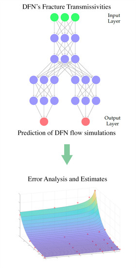
1. Introduction

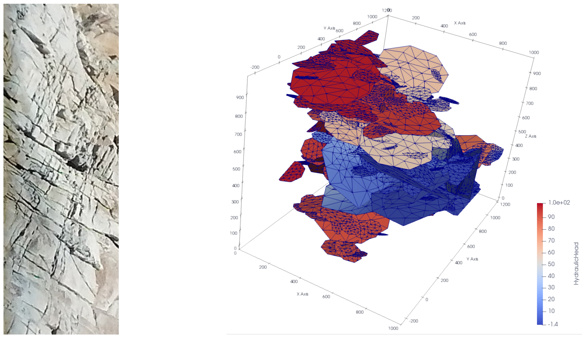
Analysis of underground flows in fractured media is relevant in several engineering fields, e.g., in oil and gas extraction, in geothermal energy production, or in the prevention of geological or water-pollution risk, to mention a few. Many possible approaches exist for modeling fractured media, and among the most used is the Discrete Fracture Network (DFN) model [1,2,3]. In this model, fractures in the rock matrix are represented as planar polygons in a three-dimensional domain that intersect each other; through the intersection segments (called “traces”), a flux exchange between fractures occurs while the 3D domain representing the surrounding rock matrix is assumed to be impermeable. On each fracture, the Darcy law is assumed to characterize the flux and head continuity and flux balance are assumed to characterize all traces.

Underground flow simulations using DFNs can be, however, a quite challenging problem in the case of realistic networks, where the computational domain is often characterized by a high geometrical complexity; in particular, fractures and traces can intersect, forming very narrow angles, or can be very close to each other. These complex geometrical characteristics make the creation of the mesh a difficult task, especially for numerical methods requiring conforming meshes. Therefore, new methods using different strategies have been proposed in the literature to avoid these meshing problems. In particular, in [4,5,6,7], the mortar method is used, eventually together with geometry modifications, while in [8,9,10], lower-dimensional problems are introduced in order to reduce the complexity. Alternatively, a new method that allowed the meshing process be considered an easy task was illustrated in [11,12,13,14,15,16,17]; in this case, the problem was reformulated as a Partial Differential Equation (PDE) constrained optimization one; thanks to this reformulation, totally non-conforming meshes are allowed on different fractures and the meshing process can be independently performed on each fracture. The simulations used in this study are performed with this approach. Other approaches can be found in [18,19,20,21].

In real-world problems, full deterministic knowledge of the hydrogeological and geometric properties of an underground network of fractures is rarely available. Therefore, these characteristics are often described through probability distributions, inferred by geological analyses of the basin [22,23,24,25]. This uncertainty about the subsurface network of fractures implies a stochastic creation of DFNs, sampling the geometric features (position, size, orientation, etc.) and hydrogeological features from the given distributions; then, the flux and transport phenomena are analyzed from a statistical point of view. For this reason, Uncertainty Quantification (UQ) analyses are required to compute the expected values and variances (i.e., the momentums) of the Quantity of Interests (QoI), e.g., the flux flowing through a section of the network. However, UQ analyses typically involve thousands of DFN simulations to obtain trustworthy values of the QoI momentums [26,27] and each simulation may have a relevant computational cost (both in terms of time and memory). Then, it is worth considering some sort of complexity reduction techniques, e.g., in order to speed up the statistical analyses, such as the multi-fidelity approach [28] or graph-based reduction techniques [29].

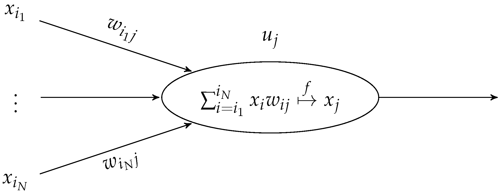
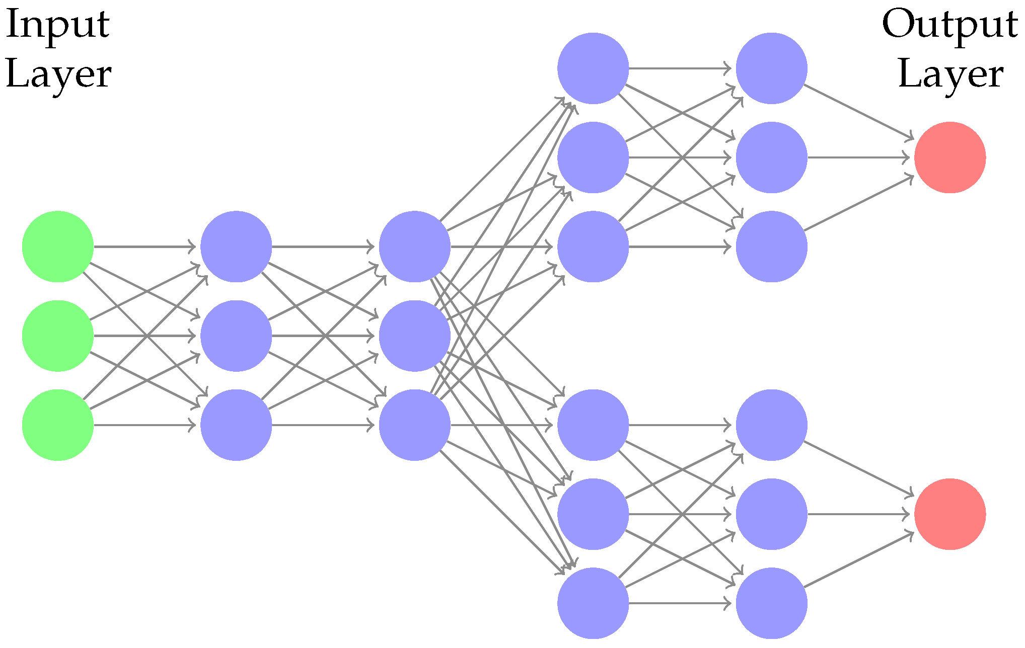
Machine Learning (ML), and in particular Neural Networks (NNs), in recent years has been proven to be a potential useful instrument for frameworks related to complexity reduction due to their negligible computational cost in making predictions. Some recent contributions involving ML and NNs applied to DFN flow simulations or UQ analysis are proposed in [30,31,32,33,34,35]. To the best of the authors’ knowledge, other than [35,36,37] there are no works in the literature that involve the use of NNs as a model reduction method for DFN simulations. In particular, in [35], multi-task deep neural networks are trained to predict the fluxes of DFNs with fixed geometry, given the fracture transmissivities. A well-trained Deep Learning (DL) model can predict the results of thousands of DFN simulations in the order of a second and, therefore, lets a user estimate the entire distribution (not only momentums) of the chosen QoI; the simulations that must be run to generate the training data are the actual computational cost. The results of [35] showed not only that NNs can be useful tools for predicting the flux values in a UQ framework but also that the quality of the flux approximation is very sensitive to some training hyperparameters. In particular, a strong dependence of the performance was observed when the training set size varied.

In this paper, we deeply investigate the dependence of the performances of a trained NN and the size of the training set required for good flux prediction on variance in the stochastic parameter of fracture transmissivities. When variability in the phenomenon increases, good training of an NN requires more and more data. If the data are generated by numerical models, a large number of simulations are necessary for the creation of the dataset involved in training the NN. Then, it can be useful to have a tool that provides an estimate of NN performances for different amounts of training data and for different values of variance in the stochastic input parameters. This issue is relevant to predict the convenience of the approach in real-world applicative situations. Indeed, we recall that the DFN simulations required to generate the training data are the only nonnegligible cost for training NNs on these problems. Therefore, it is important to provide a rule that estimates the number of simulations needed to train an NN model with good performances: if the number of simulations for NN training is less than the number required by a standard UQ analysis, it is convenient to use an NN reduced model; otherwise, other approaches can be considered.

In this work, we take into account the same flux regression problem described in [35] and we explicitly analyze the performance behavior of the NNs trained for DFN flux regression. The analysis is applied to a pair of DFN geometries and to multiple NNs with different architectures and training configurations, showing interesting behaviors that let us characterize the relationship between the number of training data, the transmissivity standard deviation, and the NN performances. From this relationship, we determine a “UQ rule” that provides an estimate of the minimum number of simulations required for training an NN with a flux approximation error less than an arbitrary $\epsilon >0$. The rule is validated on a third DFN, proving concrete efficiency and applicability to real-world problems.

The paper is organized as follows. In Section 2, we start with a brief description of the DFN numerical models and their characterization for the analyses of this work; then, we continue with a short introduction on the framework of NNs in order to better describe the concepts discussed in Section 2.2.3 that concerns the application of deep learning models for flux regression in DFNs. In Section 2.3, the performance analysis procedure used in this work is described step by step. In Section 3, we show the application of the analysis described in the previous section and the results obtained for the two test cases considered; in particular, here, we introduce interesting rules that characterize the error behaviors and that are useful for estimating the minimum number of data required for good NN training. We conclude the work with Section 4 and Section 5, where the main aspects of the obtained results are commented upon and discussed.

2. Methods

2.1. Discrete Fracture Networks

We recall here, for the reader’s convenience, the model problem of Discrete Fracture Networks (DFNs). The model is described briefly, and for full details, we point the interested reader to [3,10,11,14]. After the model description, we also introduce the main characteristics of the DFNs used for the performance analysis of Neural Networks (NNs) trained for flux regression.

2.1.1. Numerical Model and Numerical Solution

A DFN is a discrete model that describes an underground network of fractures in a rock medium. In a DFN, the network of fractures is represented as a set of intersecting two-dimensional polygons in a three-dimensional space (see Figure 1).

Each one of the polygons that stands for the network fractures was labeled with an index in a set I, and each fracture was denoted by ${\mathcal{F}}_i$, with $i\in I$; then, a DFN was given by the union ${\bigcup }_{i\in I}{\mathcal{F}}_i$ of all the fractures. The intersections between fractures of the DFN are called traces, and through them, the flow crosses the network.

The flow model we assumed in the network was a simple Darcy model, and the DFN numerical simulation consisted in finding for each $i\in I$ the hydraulic head $H_i$ of fracture ${\mathcal{F}}_i$. In our simulations, the flow was induced by a fixed pressure difference $\Delta H$ between two arbitrary surfaces of the 3D domain of the DFN. In order to solve the problem, some matching conditions were imposed at each trace of the network: we assumed the hydraulic head continuity and the flux balance. In this work, the DFN numerical simulations were computed following the approach described in [11,12], reformulating the problem as a PDE-constrained optimization one and using the finite elements as the space discretization method.

The flow simulation in a DFN was characterized by the geometry and by hydrogeological properties. In particular, for each $i\in I$, the transmissivity parameter ${\kappa }_i$ of the fracture ${\mathcal{F}}_i$ characterized the flow facilitation through the fracture. In the most general case, the fracture transmissivity ${\kappa }_i$ can be a function of the fracture points, but in this work, we considered it as a constant parameter for each fracture ${\mathcal{F}}_i$.

In this work, we trained the NN regression models to predict the fluxes exiting from the DFN given the set of transmissivities of its fractures for a fixed geometry and $\Delta H$.

2.1.2. DFN Characterization

In the problem addressed in this work, we considered two DFN geometries and the transmissivities were modelled as random variables with a known distribution.

In particular, each DFN considered in this paper was characterized by the following properties:

• A fixed geometry with $n\in \mathbb{N}$ fractures ${\mathcal{F}}_1,\dots ,{\mathcal{F}}_n$ in a cubic domain $\mathbb{D}={[0,\ell ]}^3\subset {\mathbb{R}}^3$ with edge length $\ell =1000\mathrm{m}$. The fractures were assumed to be octagons and randomly generated as in [22,23], i.e., with geometrical features such that we had the following:

  -

  The fracture radii were sampled with respect to a truncated power law distribution with exponent $\gamma =2.5$, upper cutoff $r_u=560$, and lower cutoff $r_0=50$.

  -

  The fracture orientations were sampled from a Fisher distribution with mean direction $\mathit{\mu }={[0.0065,-0.0162,0.9998]}^{\top }$ and dispersion parameter $\delta =17.8$.

  -

  The mass center of fractures were sampled with respect to a uniform distribution in $\mathbb{D}$.

• The Darcy flow model on each fracture was induced by a fixed head difference $\Delta H=10\mathrm{m}$ between the two surfaces of $\mathbb{D}$ corresponding to $x=0$ and $x=\ell$. More specifically, we imposed a Dirichlet boundary condition $H=10\mathrm{m}$ on fracture edges obtained intersecting the DFN with the plane $x=0$ and we imposed $H=0\mathrm{m}$ on the fracture edges obtained intersecting the network with the plane $x=\ell$.
• Transmissivities ${\kappa }_1,\dots ,{\kappa }_n\in \mathbb{R}$ of the n fractures were assumed to be isotropic parameters, modeled as random variables with respect to a log-normal distribution [24,25], i.e., such that

  $${log}_{10}\left({\kappa }_i\right)\sim \mathcal{N}\left(-5,\sigma \right),\mathrm{for}\mathrm{each}i=1,\dots ,n,$$

  (1)

  where $\sigma \in \mathbb{R}$ is an arbitrary parameter that characterizes the standard deviation of the transmissivity distribution.
• Due to the fixed geometry of the DFN, the fracture positions in the space did not change. Then, given the fixed pressure difference $\Delta H$, we had that the boundary fractures with flux entering and exiting the network were the ones intersecting the plane $x=0$ and the plane $x=\ell$, respectively, independently from the transmissivity values. We denoted with $m\in \mathbb{N}$ the number of boundary fractures with exiting flux.

2.2. Neural Networks

Neural Networks are powerful ML models that were first introduced more than fifty years ago (see, e.g., [38,39,40]). In the last decade, the usage of NNs has been characterized by incredible growth, thanks to new and more powerful computer hardware and the increase in available data (see Chapter 1 in [41]).

In this section, we recap briefly the main properties of NNs, and in Section 2.2.3, we describe the multi-task architecture adopted for the flux regression problem in DFNs.

2.2.1. General Concepts about Neural Networks and Learning Models

An NN, similar to most other ML models, is a parametric model ${\widehat{\mathit{F}}}_{\mathit{w}}:{\mathbb{R}}^n\to {\mathbb{R}}^m$, where the vector of parameters (also called weights) $\mathit{w}$ is adjusted through an error-minimization process in order to approximate a fixed target function $\mathit{F}:\Omega \subseteq {\mathbb{R}}^n\to {\mathbb{R}}^m$, i.e., looking for a final vector of parameters ${\mathit{w}}_{\mathit{fin}}$ such that ${\widehat{\mathit{F}}}_{{\mathit{w}}_{\mathit{fin}}}\left(\mathit{x}\right)\approx \mathit{F}\left(\mathit{x}\right)$ for each $\mathit{x}\in \Omega$. In typical ML problems, the function $\mathit{F}$ is unknown or requires high computational efforts to be executed, justifying the need to find a computationally cheap approximation of it. The parameters ${\mathit{w}}_{\mathit{fin}}$ are computed starting from a dataset of pairs:

$$\mathcal{D}=\left\{({\mathit{x}}_d,{\mathit{y}}_d=\mathit{F}\left({\mathit{x}}_d\right))\in \Omega \times {\mathbb{R}}^m|d=1,\dots ,D\right\},$$

(2)

where $D\in \mathbb{N}$ and $\mathcal{D}$ are obtained from observation of real data (when $\mathit{F}$ is unknown) or built after random sampling of D elements ${\mathit{x}}_d$ from the domain $\Omega$ and evaluating ${\mathit{y}}_d$ when $\mathit{F}$ is known but computationally expensive. The search for an optimal weight vector, such that $\mathit{F}$ is approximated by ${\widehat{\mathit{F}}}_{\mathit{w}}$, is based on a subset $\mathcal{T}\subseteq \mathcal{D}$ called the training set. The idea is to find a weight vector that minimizes an arbitrary error measure, e.g., the square of the euclidean norm $\Vert {\widehat{\mathit{F}}}_{\mathit{w}}{\left(\mathit{x}\right)-\mathit{y}\Vert }^2$ for each pair $(\mathit{x},\mathit{F}\left(\mathit{x}\right)=\mathit{y})\in \Omega \times {\mathbb{R}}^m$; to do so, in NNs typically, we solve a stochastic optimization problem of the following form:

$$\underset{\mathit{w}}{min}\left\{\mathrm{Loss}\left(\mathit{w}\right)=L({\widehat{\mathit{F}}}_{\mathit{w}},\mathcal{B})|\mathcal{B}\subseteq \mathcal{T}\right\},$$

(3)

where the subset $\mathcal{B}$, also called minibatch, is a set of $B\in \mathbb{N}$ pairs randomly sampled from $\mathcal{T}$ and $L({\widehat{\mathit{F}}}_{\mathit{w}},\mathcal{B})$ is the loss function on $\mathcal{B}$, e.g., the sum of Mean Square Errors (sMSE) over the pairs of the minibatch:

$$sMSE({\widehat{\mathit{F}}}_{\mathit{w}},\mathcal{B})=\sum _{j=1}^m\left(\frac{1}{B}\sum _{(\mathit{x},\mathit{y})\in \mathcal{B}}{\left({\widehat{y}}_j-y_j\right)}^2\right),$$

(4)

where $\widehat{\mathit{y}}:={\widehat{\mathit{F}}}_{\mathit{w}}\left(\mathit{x}\right)$ for each $\mathit{x}\in {\mathbb{R}}^n$, and ${\widehat{y}}_j$ and $y_j$ are the jth components of $\widehat{\mathit{y}}$ and $\mathit{y}$, respectively, for each $j=1,\dots ,m$ (vectors are denoted by boldface symbols).

The problem (3) is solved with arbitrary variants of the stochastic gradient descent method (see Chapter 8.3 in [41]), i.e., variants of the gradient iterative method that perform a minimization iteratively on a random minibatch $\mathcal{B}\subset \mathcal{T}$ of fixed size B at each step. In particular, the sampling of $\mathcal{B}$ at each step occurs without repetition until all the pairs $(\mathit{x},\mathit{y})\in \mathcal{T}$ have been extracted; once the pairs $(\mathit{x},\mathit{y})\in \mathcal{T}$ are finished, an epoch of the training is completed and a new one starts, until it reaches a stopping criterium. An NN model can be trained for many epochs to improve the approximation of $\mathit{F}$.

The remaining pairs of data, i.e., the pairs $(\mathit{x},\mathit{y})\in \mathcal{D}\backslash \mathcal{T}$, are used for monitoring and evaluating the quality of the NN training. Usually, the set $\mathcal{D}$ is split in three disjoint subsets:

• the training set $\mathcal{T}$ (already introduced above),
• the validation set $\mathcal{V}$, and
• the test set $\mathcal{P}$.

The validation set $\mathcal{V}$ is often the smallest of the three subsets, and it is used to measure the approximation error of ${\widehat{\mathit{F}}}_{\mathit{w}}$ at the end of each training epoch; the test set $\mathcal{P}$, on the contrary, is often bigger than $\mathcal{V}$ (and sometimes also bigger than $\mathcal{T}$), and it is used to measure the approximation quality of the trained NN on new data that the model never used during the training phase. Then, $\mathcal{P}$ is useful to understand if the NN is a good approximation of the target function for new input data, whereas $\mathcal{V}$ is useful to monitor the training activity and to define the proper stopping criteria for avoiding underfitting/overfitting problems (see Chapter 5.2 in [41]).

2.2.2. Neural Network Structure

The structure of an NN is what actually makes it different from other ML models. An NN is a learning algorithm that can be described through an oriented weighted graph $(U,A)$, where U is the set of nodes and A is the set of edges, i.e., the set of ordered pairs of nodes $a_{ij}=(u_i,u_j)\in A\subseteq U\times U$n each one endowed with a weight $w_{ij}\in \mathbb{R}$.

Each node of an NN, also called a unit or a neuron, can receive signals either from other nodes (through the edges) or from one external source; in the latter case, the unit is defined as the input unit of the NN and it returns as output the same signal received as an input. Each non-input unit $u_j\in U$ performs arbitrary fixed operations on the input signals $x_{i_1},\dots ,x_{i_N}$ (sent by units $u_{i_1},\dots ,u_{i_N}\in U$) and returns an output signal $x_j$. Typically, a unit is characterized as in Figure 2, i.e., with output signal $x_j$ such that

$$x_j=f\left(\sum _{i\in \{i_1,\dots ,i_N\}}{x}_i{w}_{ij}\right),$$

(5)

where f is an arbitrary function called the activation function.

If the output $x_j$ of $u_j$ is sent only to other units of the NN, then $u_j$ is defined as a hidden unit; otherwise, if the signal $x_j$ is sent “outside” as a general output of the NN model, then $u_j$ is defined as an output unit.

One special type of hidden unit is the bias units that are characterized by a fixed unit output. For this reason, Equation (5) is rewritten with a different notation that highlights the action of the bias unit:

$$x_j=f\left(\sum _{\begin{array}{c}i\in \{i_1,\dots ,i_N\}\\ i\ne \mathit{bias}\end{array}}{x}_i{w}_{ij}+b_j\right),$$

(6)

where $b_j$ is the weight of the edge $(u_{\mathit{bias}},u_j)$ and $u_{\mathit{bias}}\in U$ is a bias unit connected to $u_j$. Even if it is not forbidden, in practice, no more than one bias unit is connected to one hidden or output unit.

We conclude this brief description of NN structure by introducing the concept of “layers” for NNs. NN architectures organize their units in subsets that interact with each other; these subsets are called layers and can be divided in three main types (as the units): the input layers, the hidden layers, and the output layers.

The simplest type of hidden and output layers are the so-called fully connected layers. A fully connected layer L that receives signals from a layer I is characterized by the fact that each unit in L is connected to all the units in I and that all the units in L have the same activation function f; then, assuming that all the units in L are characterized by (6), the layer action of the output signals from I can be described as the function $\mathcal{L}$ such that

$${\mathit{x}}^{\left(L\right)}=\mathcal{L}\left({\mathit{x}}^{\left(I\right)}\right)=\mathit{f}\left(W^{\top }{\mathit{x}}^{\left(I\right)}+\mathit{b}\right),$$

(7)

where

• ${\mathit{x}}^{\left(L\right)}\in {\mathbb{R}}^M$ and ${\mathit{x}}^{\left(I\right)}\in {\mathbb{R}}^N$ are the vectors of the output signals of L and I, respectively;
• $\mathit{f}:{\mathbb{R}}^M\to {\mathbb{R}}^M$ is the element-wise application of the activation function f of the layer units;
• $W\in {\mathbb{R}}^{N\times M}$ is the weight matrix with entry weights $w_{ij}$, corresponding to the edge that connects unit $u_i$ of I to unit $u_j$ of L; and
• $\mathit{b}\in {\mathbb{R}}^M$ is the vector of bias weights for the M units of L.

See Figure 3 for a graphical representation of a fully connected layer.

Layer formulation in NNs is extremely useful when better describing the function ${\widehat{\mathit{F}}}_{\mathit{w}}$ as a composition of layer functions and for NN implementation in computer programs. The representation of ${\widehat{\mathit{F}}}_{\mathit{w}}$ as a composition of functions is used to build a computational graph that is extremely useful in speeding up the computation of both NN outputs and the gradient of the loss function during the training phase. For more details about these properties, see Chapter 6 in [41].

2.2.3. Deep Learning Models for Flux Regression in DFNs

Let us consider a DFN with a geometry defined as in Section 2.1.2, where n is the number of fractures and m is the number of boundary fractures with exiting flux; we recall that the case has fixed geometry and that only the fracture transmissivities change (see (1)). For each vector of transmissivity samples $\mathit{\kappa }={[{\kappa }_1,\dots ,{\kappa }_n]}^{\top }$, we can run a flow simulation for the given DFN and compute the m fluxes $\mathit{\phi }={[{\phi }_1,\dots ,{\phi }_m]}^{\top }$ of the m boundary outflowing-flux fractures. Let $\mathit{F}:{\mathbb{R}}^n\to {\mathbb{R}}^m$ be a function related to the given DFN such that

$$\mathit{F}\left(\mathit{\kappa }\right)=\mathit{\phi },$$

(8)

for each $\mathit{\kappa }\in {\mathbb{R}}^n$ sampled following (1); then, we want to define a multi-task architecture for Deep Neural Network (DNN) models able to approximate $\mathit{F}$, i.e., able to predict the corresponding fluxes $\mathit{\phi }\in {\mathbb{R}}^m$ for each transmissivity vector $\mathit{\kappa }\in {\mathbb{R}}^n$ in the input. The DFN flow simulations are performed using the GEO++ software [42], based on a PDE-constrained reformulation of the problem, using finite elements for the spatial discretization. For further details, we point the interested reader to [11,14,42].

For the DNN models of this work, we adopt a multi-task architecture (see Chapter 7.7 in [41]) of the same structure described in [35]. Given a fixed hyperparameter $\alpha \in \mathbb{N}$ and the target function $\mathit{F}$, we define the DNN multi-task architecture ${\mathcal{A}}_{\alpha }$ (see Figure 4) such that

• ${\mathcal{A}}_{\alpha }$ has one input layer $L_0$ of n units;
• the input layer $L_0$ is fully connected to the first layer $L_1$ of a sequence of $\alpha$ fully connected layers: $(L_1,\dots ,L_{\alpha })$. All the layers of the sequence have n units characterized by the softplus activation function (i.e., $f\left(x\right)=log(1+e^x)$);
• let us consider m sequences of fully connected layers $(L_{\alpha +1}^{\left(j\right)},\dots ,L_{2\alpha }^{\left(j\right)})$, for each $j=1,\dots ,m$; then, the layer $L_{\alpha }$ is fully connected to each one of the first layers $L_{\alpha +1}^{\left(j\right)}$ of these sequences. All the layers $(L_{\alpha +1}^{\left(j\right)},\dots ,L_{2\alpha }^{\left(j\right)})$, for each $j=1,\dots ,m$, have n units characterized by the softplus activation function; and
• for each $j=1,\dots ,m$, the layer $L_{2\alpha }^{\left(j\right)}$ is fully connected to an output layer $L_{2\alpha +1}^{\left(j\right)}$ made of only one linear unit.

We can easily see that the characteristic function of a DNN model with architecture ${\mathcal{A}}_{\alpha }$ accepts n inputs and returns m outputs; then, it is a function ${\widehat{\mathit{F}}}_{\mathit{w}}:{\mathbb{R}}^n\to {\mathbb{R}}^m$, and the NN can be trained for approximating the function $\mathit{F}$.

In order to evaluate the quality of the approximation, for each outflow fracture, we consider an error measure that evaluates the relative distance between the flux estimated by the NN and the real flux. Let us assume that we have a trained DNN with function ${\widehat{\mathit{F}}}_{\mathit{w}}$ approximating $\mathit{F}$; then, the chosen error measure is the following:

• relative error: for each $\mathit{\kappa }\in {\mathbb{R}}^n$, we can measure the vector of prediction errors normalized by the actual total exiting flux, i.e., the vector

  $$\mathit{e}\left(\kappa \right):=\frac{1}{{\sum }_{j=1}^m{\phi }_j}\left[\right|{\phi }_1-{\widehat{\phi }}_1|,\dots ,|{\phi }_m-{\widehat{\phi }}_m{\left|\right]}^{\top },$$

  (9)

  where $\widehat{\mathit{\phi }}:={\widehat{\mathit{F}}}_{\mathit{w}}\left(\mathit{\kappa }\right)={[{\widehat{\phi }}_1,\dots ,{\widehat{\phi }}_m]}^{\top }$ is the flux prediction for $\mathit{\kappa }$. Then, given the input $\mathit{\kappa }$, for each $j=1,\dots ,m$, the jth element of error (9) tells us how much the prediction for the jth exiting flux differs from the original value, represented as a fraction of the total flux outflowing from the DFN.

The errors introduced above, are very useful in studying the prediction ability of a flux regression NN. However, in order to directly compare the predictions of different NNs, we need to define some cumulative scalar values that summarize the approximation quality of the NN models. Then, we introduce a quantity that is obtained from the aggregation of (9) once an arbitrary test set $\mathcal{P}$ of pairs $(\mathit{\kappa },\mathit{\phi })$ is given. This quantity is

• average mean relative error:

  $$E\left(\mathcal{P}\right):=\frac{1}{\left|\mathcal{P}\right|}\sum _{(\mathit{\kappa },\mathit{\phi })\in \mathcal{P}}\frac{1}{m}\sum _{j=1}^m{e}_j\left(\mathit{\kappa }\right),$$

  (10)

  where $e_j\left(\mathit{\kappa }\right)$ is the jth element of the vector $\mathit{e}\left(\mathit{\kappa }\right)$. For simplicity, from now on, we will call the quantity $E\left(\mathcal{P}\right)$ simply average error instead of average mean relative error.

2.3. Performance Analysis of Deep Learning Models for Flux Regression

In Section 2.1 and Section 2.2, we introduced all the notions needed to analyze the performances of multi-task Deep Learning (DL) models trained to predict the fluxes exiting from a DFN. In [35], the NN sensitivity to the cardinality of the training set $\mathcal{T}$ was noticed, but in those cases, a fixed value $\sigma =1/3$ for (1) was chosen. In this work, we deeply investigate this sensitivity, quantifying it through the measurement of average errors varying the available number of training data and the sparsity of the data itself.

The analysis performed in this paper compares the average errors $E\left(\mathcal{P}\right)$ of a set of NNs with a common architecture ${\mathcal{A}}_{\alpha }$ and the same configuration of training hyperparameters and functions but trained on different training data; in particular, the differences between the training data are characterized by two hyperperparameters:

• the parameter $\sigma \in {\mathbb{R}}_{\ge 0}$, characterizing the standard deviation of the transmissivity distribution (see (1)). This parameter varies among a discrete and finite set of values $\Sigma$, arbitrarily chosen;
• the number $\vartheta \in \mathbb{N}$ of data $(\mathit{\kappa },\mathit{\phi })$ used for training the NN, i.e., the sum of the training set and validation set cardinalities:

  $$\vartheta :=\left|\mathcal{T}\right|+\left|\mathcal{V}\right|.$$

  (11)
  Similar to $\sigma$, this parameter varies among a discrete and finite set of values $\Theta$, arbitrarily chosen;

In other words, the analysis procedure consists of training $\left(\right|\Sigma |·|\Theta \left|\right)$ times a fixed untrained NN, each time with respect to a set of training data characterized by a different combination of hyperparameters $(\sigma ,\vartheta )\in \Sigma \times \Theta$ (i.e., with different size $\vartheta$ and different sparsity, dependent from $\sigma$); then, the performances (average errors) of all the new $\left(\right|\Sigma |·|\Theta \left|\right)$ trained NNs are measured on test sets of the same size and compared, searching for the behavior of average errors with respect to values of $\sigma$ and $\vartheta$.

2.3.1. Performance Analysis: Method Description

Let us consider a DFN of the type described in Section 2.1.2 and let

$$\Sigma =\{{\sigma }_1,\dots ,{\sigma }_s\}\subset {\mathbb{R}}_{\ge 0}$$

(12)

be the set of values for the distribution parameter $\sigma$ that we want to consider for the NN performance analysis; similarly, let

$$\Theta =\{{\vartheta }_1,\dots ,{\vartheta }_t\}\subset \mathbb{N}$$

(13)

be the set of values for the number of training data $\vartheta$ considered, and let $\rho \in \mathbb{N}$ be the chosen cardinality of the test set $\mathcal{P}$ used for measuring the average errors and the mean divergences.

The method that we use in this work in order to measure and compare the NN performances in flux regression problems for DFNs is characterized by the following steps:

• Select a DFN, generated as described in Section 2.1.2, with n fractures and where m of them have exiting fluxes.
• Define the arbitrary sets of values $\Sigma$ and $\Theta$ for the hyperparameters that characterize the analysis.
• Choose the cardinality $\rho =\left|\mathcal{P}\right|$ of the test set.
• For each $\sigma \in \Sigma$, generate a set of $\delta \in \mathbb{N}$ transmissivity vectors

  $$K_{\sigma }=\{{\mathit{\kappa }}_1,\dots ,{\mathit{\kappa }}_{\delta }\}\subset {\mathbb{R}}^n,$$

  (14)

  where $\delta :=(max(\Theta )+\rho )$ and, for each $\mathit{\kappa }\in K_{\sigma }$, the transmissivity vector elements have been sampled following (1).
• For each $\sigma \in \Sigma$, for each $\mathit{\kappa }\in K_{\sigma }$, compute the corresponding flux vector $\mathit{\phi }=\mathit{F}\left(\mathit{\kappa }\right)$ running a DFN flow simulation. Then, for each $\sigma \in \Sigma$, we obtain a dataset

  $${\mathcal{D}}_{\sigma }=\left\{({\mathit{\kappa }}_i,{\mathit{\phi }}_i)\in K_{\sigma }\times {\mathbb{R}}^m|{\mathit{\phi }}_i=\mathit{F}\left({\mathit{\kappa }}_i\right),\forall i=1,\dots ,\delta \right\}.$$

  (15)
• For each $\sigma \in \Sigma$, create a test set ${\mathcal{P}}_{\sigma }$ with a random sampling of $\rho$ pairs from ${\mathcal{D}}_{\sigma }$.
• Choose a value $\alpha \in \mathbb{N}$, and build a not trained NN $\mathcal{N}$ with architecture ${\mathcal{A}}_{\alpha }$.
• For each $\sigma \in \Sigma$, for each $\vartheta \in \Theta$, sample randomly a number $\vartheta$ of pairs $(\mathit{\kappa },\mathit{\phi })$ from ${\mathcal{D}}_{\sigma }\backslash {\mathcal{P}}_{\sigma }$ (i.e., the dataset without the test set). We decides to use $20\%$ of the $\vartheta$ sampled pairs as the validation set ${\mathcal{V}}_{\sigma }^{\vartheta }$ and the remaining $80\%$ as the training set ${\mathcal{T}}_{\sigma }^{\vartheta }$.
• For each pair $(\sigma ,\vartheta )\in \Sigma \times \Theta$, train the untrained NN $\mathcal{N}$ using the data of ${\mathcal{T}}_{\sigma }^{\vartheta }$ and ${\mathcal{V}}_{\sigma }^{\vartheta }$, obtaining a trained NN ${\mathcal{N}}_{\sigma }^{\vartheta }$. For all the cases, the training is characterized by the same hyperparameters and functions arbitrarily chosen.
• For each pair $(\sigma ,\vartheta )\in \Sigma \times \Theta$, measure the quantity $E_{\sigma }^{\vartheta }$ that is the average error $E\left({\mathcal{P}}_{\sigma }\right)$ computed for the NN ${\mathcal{N}}_{\sigma }^{\vartheta }$.
• Analyze the set of points

  $$\mathrm{E}:=\left\{(\sigma ,\vartheta ,E_{\sigma }^{\vartheta })\in \Sigma \times \Theta \times \mathbb{R}\right\},$$

  (16)

  and then find the best fitting function $\widehat{E}:{\mathbb{R}}^2\to \mathbb{R}$ with respect to the points in $\mathrm{E}$ such that they characterize the average error as a function of the parameters $\sigma$ and $\vartheta$.

2.3.2. Training Hyperparameters and Functions

For step 9 of the method described above, we talk about a fixed and arbitrary configuration of the hyperparameters and functions of the training phase. In particular, in this work, we perform the analysis considering two cases with two fixed configurations that are different only for the minibatch size adopted; we have that the first configuration is characterized by a minibatch size $\left|\mathcal{B}\right|=10$ while the second one has a minibatch size $\left|\mathcal{B}\right|=30$.

Let $\beta$ be a parameter denoting which training configuration we choose; then, $\beta =1$ represents the choice for the first configuration ($\left|\mathcal{B}\right|=10$) and $\beta =2$ represents the choice for the second configuration ($\left|\mathcal{B}\right|=30$). All the other properties of the training configurations are the same for both the cases $\beta =1$ and $\beta =2$ and are as follows:

• input data preprocessing: the input data are transformed applying first the function ${log}_{10}$ (element-wise) and then the z-normalization [43];
• output data preprocessing: the output data are rescaled by a factor equal to ${10}^6$;
• layer-weights initialization: Glorot uniform distribution [44];
• biases initialization: zeroes;
• maximum number of epochs: 1000;
• regularization methods: early stopping, Chapter 7.8 in [41] (patience parameter $p=150$);
• optimization algorithm: Adam [45] (learning rate $ϵ=0.001$, first moment decay parameter ${\gamma }_1=0.9$, and second moment decay parameter ${\gamma }_2=0.999$);
• loss function: sMSE (see (4)).

The shared hyperparameters and functions chosen for the configurations $\beta =1,2$ consist mainly in the default options provided by most of the frameworks for NN implementation; indeed, in this analysis, we focus our attention on the effects of the parameters $\sigma$ and $\vartheta$ on the NNs and, therefore, we choose standard training configurations that should grant a reasonable training quality.

3. Results

Here, we show the application of the performance analysis method described in Section 2.3 on two test cases. In particular, we consider two DFNs, DFN158, and DFN395, generated with respect to the characterization of Section 2.1.2; the total number of fractures n is equal to 158 and 395 for DFN158 and DFN395, respectively, and the number of outflux fracture m is equal to 7 and 13 for DFN158 and DFN395, respectively.

For each of these two DFNs, we train three different NNs with architectures ${\mathcal{A}}_{\alpha }$ (see Section 2.2.3) for each $\alpha =1,2,3$ and with respect to the two training configurations $\beta =1$ and $\beta =2$ (see Section 2.3.2); then, we have a total number of six trained NNs, one for each $(\alpha ,\beta )$ combination, for both DFN158 and DFN395. Moreover, we fixed the values $\rho =3000$ for the test set cardinality and the set $\Theta =\{500,1000,2000,4000,7000\}$ of training-validation set cardinalities $\vartheta$. For the two DFNs considered, we define the set of distribution parameters $\sigma$ such that

• DFN158:$\Sigma =\{1/5=0.20,1/4=0.25,1/3\approx 0.33,2/5=0.40,1/2=0.50,0.70\}$.
• DFN395:$\Sigma =\{1/5=0.20,1/3\approx 0.33,1/2=0.5\}.$

In total, for the following analyses, we trained 180 NNs for DFN158 (30 for each $(\alpha ,\beta )$ case) and 90 NNs for DFN395 (15 for each $(\alpha ,\beta )$ case); the reason for the smaller set $\Sigma$ and, therefore, a smaller number of trainings for DFN395 depends on the more expensive DFN simulations (with respect to the ones of DFN158) that are needed for the creation of the dataset ${\mathcal{D}}_{\sigma }$ (see step 5 of the method in Section 2.3). The results found for the two DFNs are in very good agreement.

The analysis was performed for different combinations of the parameters $\alpha$ and $\beta$ in order to show that the results found are general for the family of NNs. After these performance analyses, in Section 3.3, we describe the rules for the best choice of $\vartheta$ value given a $\sigma$ value.

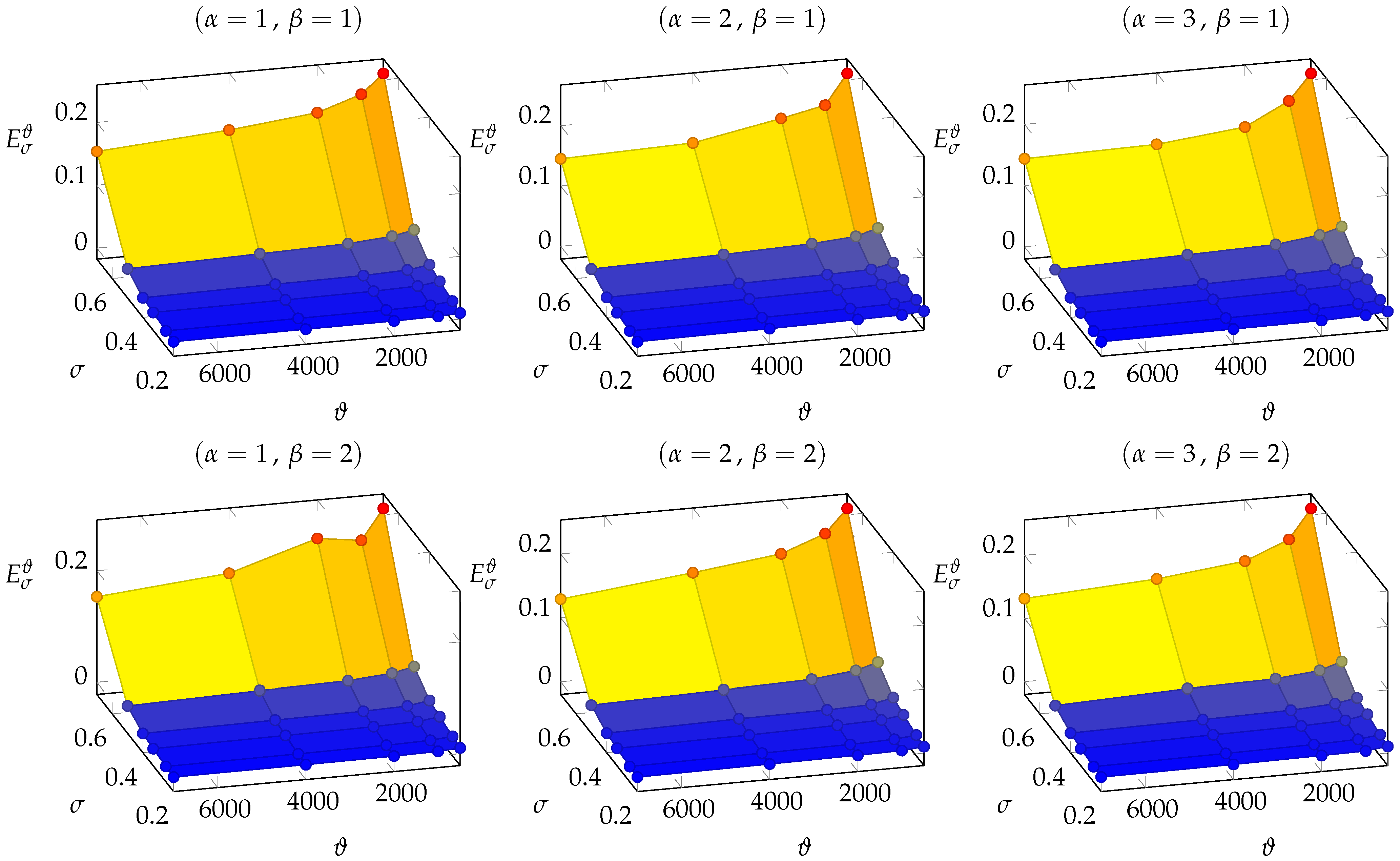
3.1. DFN158

Given the 180 trained NNs with respect to the datasets ${\mathcal{T}}_{\sigma }^{\vartheta }$ and ${\mathcal{V}}_{\sigma }^{\vartheta }$ of DFN158, we analyzed the set of points $\mathrm{E}$ (see (16)) for any fixed combination $(\alpha ,\beta )\in \{1,2,3\}\times \{1,2\}$; this set of points is described in

Table 1. DFN158. Table of the $E_{\sigma }^{\vartheta }$ values, varying $(\sigma ,\vartheta )\in \Sigma \times \Theta$, for each NN of architecture ${\mathcal{A}}_{\alpha }$ trained with configuration $\beta$, for each $\alpha =1,2,3$, and for each $\beta =1,2$.

${\mathit{E}}_{\mathit{\sigma }}^{\mathit{\vartheta }}$		$\mathit{\alpha }=1$					$\mathit{\alpha }=2$					$\mathit{\alpha }=3$
	$\mathbf{\sigma }/\mathbf{\vartheta }$	500	1000	2000	4000	7000	500	1000	2000	4000	7000	500	1000	2000	4000	7000
$\beta =1$	0.20	0.0097	0.0076	0.0066	0.0063	0.0055	0.0104	0.0074	0.0065	0.0046	0.0028	0.0106	0.0077	0.0055	0.0047	0.0036
	0.25	0.0132	0.0097	0.0086	0.0080	0.0073	0.0129	0.0099	0.0085	0.0068	0.0044	0.0134	0.0103	0.0081	0.0068	0.0051
	∼0.33	0.0190	0.0148	0.0129	0.0119	0.0109	0.0190	0.0148	0.0128	0.0109	0.0081	0.0205	0.0154	0.0130	0.0107	0.0084
	0.40	0.0248	0.0196	0.0171	0.0160	0.0136	0.0263	0.0184	0.0166	0.0150	0.0119	0.0264	0.0193	0.0166	0.0146	0.0120
	0.50	0.0494	0.0423	0.0369	0.0335	0.0288	0.0515	0.0410	0.0355	0.0308	0.0267	0.0539	0.0434	0.0345	0.0307	0.0262
	0.70	0.2366	0.2066	0.1837	0.1687	0.1538	0.2434	0.1942	0.1787	0.1515	0.1451	0.2406	0.1991	0.1629	0.1477	0.1438
$\beta =2$	0.20	0.0103	0.0077	0.0064	0.0055	0.0047	0.0103	0.0072	0.0062	0.0049	0.0033	0.0106	0.0066	0.0057	0.0042	0.0032
	0.25	0.0136	0.0102	0.0085	0.0074	0.0063	0.0131	0.0097	0.0078	0.0068	0.0047	0.0139	0.0096	0.0077	0.0063	0.0043
	∼0.33	0.0199	0.0150	0.0128	0.0115	0.0093	0.0195	0.0147	0.0126	0.0010	0.0079	0.0206	0.0140	0.0116	0.0103	0.0074
	0.40	0.0258	0.0195	0.0172	0.0157	0.0133	0.0262	0.0184	0.0162	0.0149	0.0113	0.0259	0.0199	0.0158	0.0137	0.0115
	0.50	0.0512	0.0428	0.0366	0.0336	0.0278	0.0506	0.0408	0.0334	0.0296	0.0247	0.0523	0.0412	0.0345	0.0318	0.0242
	0.70	0.2650	0.2115	0.2221	0.1740	0.1534	0.2304	0.1942	0.1689	0.1518	0.1293	0.2329	0.1871	0.1591	0.1436	0.1315

and illustrated in Figure 5.

For the average errors $E_{\sigma }^{\vartheta }$, we observed the following behavior characteristics:

• The general trend of $E_{\sigma }^{\vartheta }$ decreases with respect to $\vartheta$ and increases with respect to $\sigma$. Indeed, higher values of $\vartheta$ provide more data for better training the NN whereas higher values for $\sigma$ mean a larger variance for input data and, therefore, a more difficult target function $\mathit{F}$ to be learned.
• Keeping the value of $\sigma$ fixed, we observed that, in the logarithmic scale, the values of $E_{\sigma }^{\vartheta }$ are inversely proportional to $\vartheta$ (see Figure 6-left).
• Keeping the value of $\vartheta$ fixed, we observe that, in the logarithmic scale, the values of $E_{\sigma }^{\vartheta }$ increase with respect to $\sigma$ (see Figure 6-right), with an almost quadratic behavior with respect to $\sigma$.

The numerical results and these observations actually suggest that the performances of an NN for flux regression seem to be characterized by well-defined hidden rules. Therefore, as proposed at the end of step 11 of the method, we sought a function $\widehat{E}(\sigma ,\vartheta )$ such that

$$\widehat{E}(\sigma ,\vartheta )\approx E_{\sigma }^{\vartheta },$$

(17)

for each $(\sigma ,\vartheta )\in \Sigma \times \Theta$.

Taking into account the observations at items 2 and 3, we decided to look for $\widehat{E}(\sigma ,\vartheta )$ among the set of exponential functions characterized by exponents inversely proportional to $\vartheta$ and proportional to $\sigma$ with linear or quadratic behavior, i.e., functions with the following expressions:

$$g_1(\sigma ,\vartheta )=e^{(c_1+\frac{c_2}{\vartheta }+c_3\sigma +c_4{\sigma }^2)}\mathrm{and}{g}_2(\sigma ,\vartheta )=e^{(c_1+\frac{c_2}{\vartheta }+c_3\sigma )},$$

(18)

where $c_1,c_3\in \mathbb{R}$ and $c_2,c_4\in {\mathbb{R}}_{\ge 0}$ are parameters of the functions.

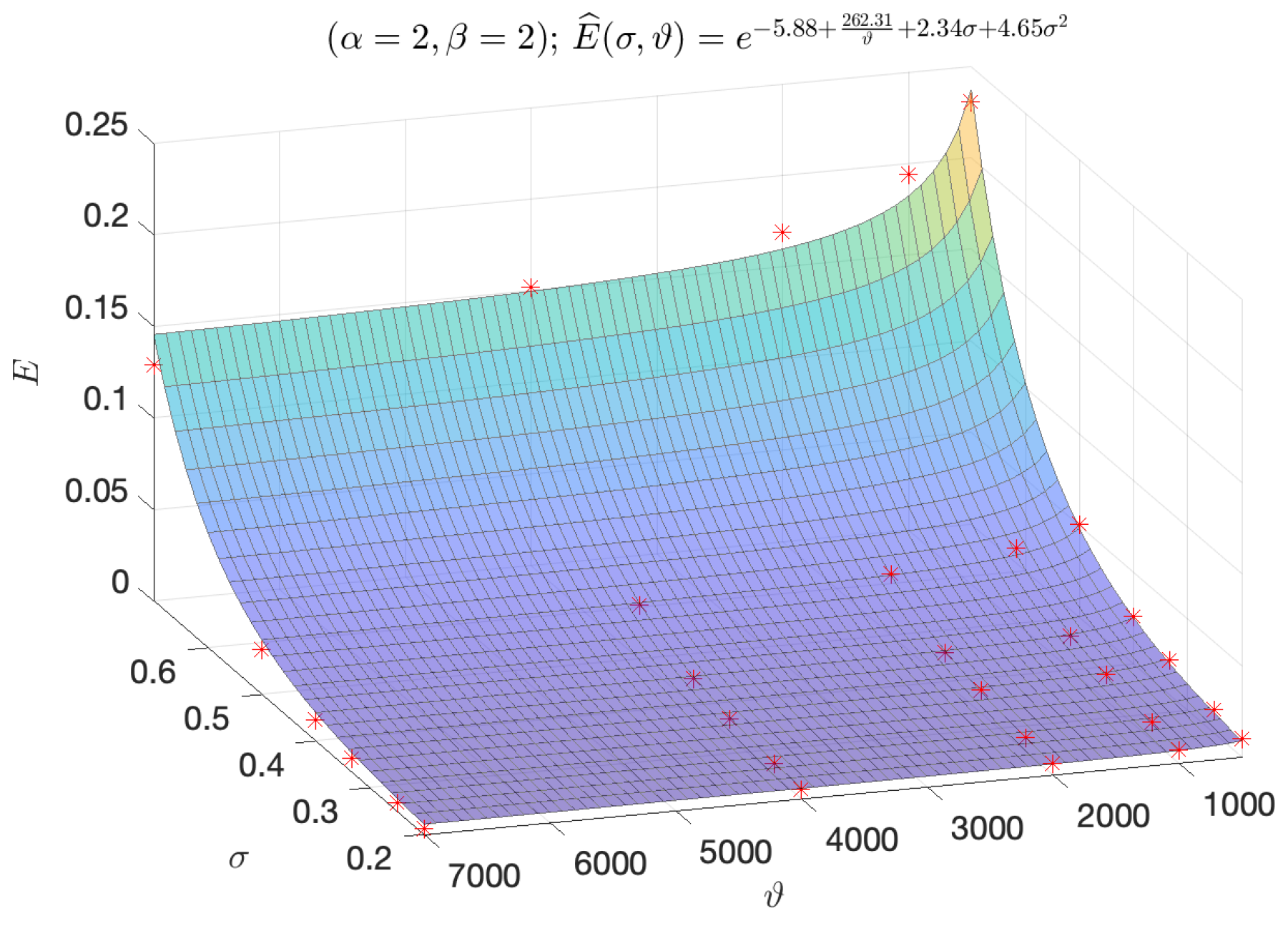
Through a least square error minimization process, we found the best-fitting coefficients for the functions (18) with respect to the data points $E_{\sigma }^{\vartheta }$ (see

Table 2. DFN158. Mean Square Error (MSE) and coefficients of the least square minimization with respect to $E_{\sigma }^{\vartheta }$.

		$\mathit{\alpha }=1$					$\mathit{\alpha }=2$					$\mathit{\alpha }=3$
	${\mathit{E}}_{\mathit{\sigma }}^{\mathit{\vartheta }}$	MSE	${\mathit{c}}_{\mathbf{1}}$	${\mathit{c}}_{\mathbf{2}}$	${\mathit{c}}_{\mathbf{3}}$	${\mathit{c}}_{\mathbf{4}}$	MSE	${\mathit{c}}_{\mathbf{1}}$	${\mathit{c}}_{\mathbf{2}}$	${\mathit{c}}_{\mathbf{3}}$	${\mathit{c}}_{\mathbf{4}}$	MSE	${\mathit{c}}_{\mathbf{1}}$	${\mathit{c}}_{\mathbf{2}}$	${\mathit{c}}_{\mathbf{3}}$	${\mathit{c}}_{\mathbf{4}}$
$\beta =1$	$g_1$	$1.848\times {10}^{-2}$	$-5.678$	$206.3$	$1.869$	$5.139$	$1.802\times {10}^{-2}$	$-5.928$	$261.0$	$2.551$	$4.535$	$1.778\times {10}^{-2}$	$-5.969$	$276.3$	$2.843$	$4.129$
	$g_2$	$2.255\times {10}^{-2}$	$-7.188$	$206.3$	$7.649$	-	$2.109\times {10}^{-2}$	$-7.262$	$260.9$	$7.628$	-	$2.054\times {10}^{-2}$	$-7.177$	$276.2$	$7.457$	-
$\beta =2$	$g_1$	$4.014\times {10}^{-2}$	$-5.652$	$233.1$	$1.515$	$5.742$	$2.521\times {10}^{-2}$	$-5.884$	$262.3$	$2.342$	$4.653$	$1.709\times {10}^{-2}$	$-6.084$	$285.8$	$3.171$	$3.785$
	$g_2$	$4.262\times {10}^{-2}$	$-7.356$	$233.0$	$7.966$	-	$2.757\times {10}^{-2}$	$-7.248$	$262.2$	$7.545$	-	$1.936\times {10}^{-2}$	$-7.190$	$285.5$	$7.399$	-

). Looking at the results, we see that the observation made at item 3 concerning the quadratic behavior of $E_{\sigma }^{\vartheta }$ with respect to $\sigma$ is confirmed; indeed, the approximation error of $g_1$ is always smaller than the one of $g_2$ (with a nonzero coefficient $c_4$). Then, we have that a good function $\widehat{E}(\sigma ,\vartheta )$ for the characterization of the average errors is

$$\widehat{E}(\sigma ,\vartheta ):=e^{({\widehat{c}}_1+\frac{{\widehat{c}}_2}{\vartheta }+{\widehat{c}}_3\sigma +{\widehat{c}}_4{\sigma }^2)},$$

(19)

where ${\widehat{c}}_1,\dots ,{\widehat{c}}_4$ are the fixed parameters obtained with the least square minimization.

We conclude this section with a visual example (Figure 7) of the fitting quality of $\widehat{E}(\sigma ,\vartheta )$ for the values $E_{\sigma }^{\vartheta }$ of the case $(\alpha =2,\beta =2)$.

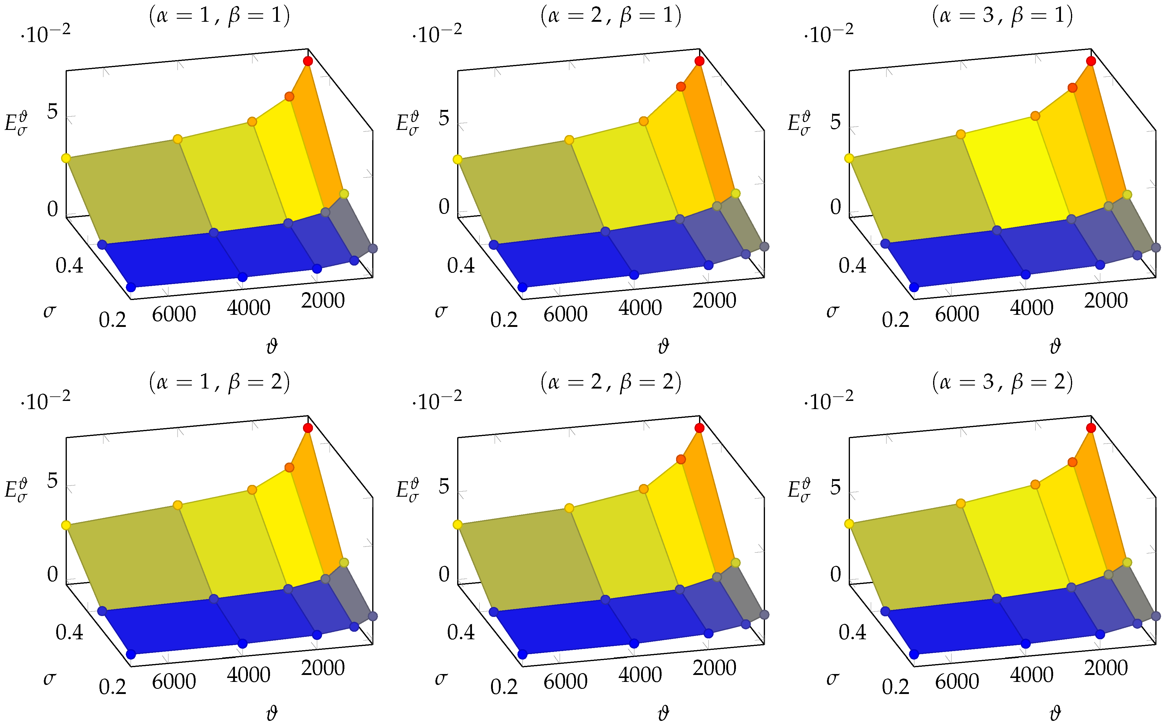
3.2. DFN395

Given the 90 trained NNs with respect to the datasets ${\mathcal{T}}_{\sigma }^{\vartheta }$ and ${\mathcal{V}}_{\sigma }^{\vartheta }$ of DFN395, we analyzed the set of points $\mathrm{E}$ for any fixed combination $(\alpha ,\beta )\in \{1,2,3\}\times \{1,2\}$. This set of points is described in

Table 3. DFN395. Table of the $E_{\sigma }^{\vartheta }$ values, varying $(\sigma ,\vartheta )\in \Sigma \times \Theta$, for each NN of architecture ${\mathcal{A}}_{\alpha }$ trained with configuration $\beta$, for each $\alpha =1,2,3$, and for each $\beta =1,2$.

${\mathit{E}}_{\mathit{\sigma }}^{\mathit{\vartheta }}$		$\mathit{\alpha }=1$					$\mathit{\alpha }=2$					$\mathit{\alpha }=3$
	$\mathbf{\sigma }/\mathbf{\vartheta }$	500	1000	2000	4000	7000	500	1000	2000	4000	7000	500	1000	2000	4000	7000
$\beta =1$	0.20	0.0132	0.0079	0.0055	0.0047	0.0046	0.0143	0.0110	0.0067	0.0050	0.0037	0.0145	0.0110	0.0073	0.0056	0.0040
	∼0.33	0.0226	0.0140	0.0102	0.0087	0.0078	0.0238	0.0176	0.0122	0.0090	0.0072	0.0243	0.0185	0.0128	0.0102	0.0083
	0.50	0.0673	0.0500	0.0389	0.0334	0.0288	0.0729	0.0594	0.0418	0.0350	0.0297	0.0761	0.0614	0.0467	0.0399	0.0318
$\beta =2$	0.20	0.0124	0.0077	0.0052	0.0041	0.0039	0.0141	0.0096	0.0063	0.0044	0.0041	0.0135	0.0102	0.0060	0.0045	0.0043
	∼0.33	0.0217	0.0139	0.0103	0.0086	0.0075	0.0230	0.0158	0.0106	0.0087	0.0075	0.0235	0.0175	0.0120	0.0094	0.0080
	0.50	0.0692	0.0490	0.0389	0.0343	0.0290	0.0738	0.0569	0.0419	0.0349	0.0312	0.0744	0.0558	0.0449	0.0379	0.0320

and illustrated in Figure 8.

Looking at the results in

Table 4. DFN395. MSE and coefficients of the least square minimization with respect to $E_{\sigma }^{\vartheta }$.

		$\mathit{\alpha }=1$					$\mathit{\alpha }=2$					$\mathit{\alpha }=3$
	${\mathit{E}}_{\mathit{\sigma }}^{\mathit{\vartheta }}$	MSE	${\mathit{c}}_{\mathbf{1}}$	${\mathit{c}}_{\mathbf{2}}$	${\mathit{c}}_{\mathbf{3}}$	${\mathit{c}}_{\mathbf{4}}$	MSE	${\mathit{c}}_{\mathbf{1}}$	${\mathit{c}}_{\mathbf{2}}$	${\mathit{c}}_{\mathbf{3}}$	${\mathit{c}}_{\mathbf{4}}$	MSE	${\mathit{c}}_{\mathbf{1}}$	${\mathit{c}}_{\mathbf{2}}$	${\mathit{c}}_{\mathbf{3}}$	${\mathit{c}}_{\mathbf{4}}$
$\beta =1$	$g_1$	$7.057\times {10}^{-3}$	$-5.638$	$417.8$	$0.0002$	$8.544$	$1.289\times {10}^{-2}$	$-5.531$	$422.0$	$0.0001$	$8.459$	$1.236\times {10}^{-2}$	$-5.465$	$391.0$	$\sim {10}^{-5}$	$8.596$
	$g_2$	$8.431\times {10}^{-3}$	$-6.839$	$417.9$	$6.665$	-	$1.402\times {10}^{-2}$	$-6.718$	$422.0$	$6.596$	-	$1.358\times {10}^{-2}$	$-6.675$	$390.9$	$6.711$	-
$\beta =2$	$g_1$	$5.874\times {10}^{-3}$	$-5.719$	$426.4$	$0.0006$	$8.872$	$9.826\times {10}^{-3}$	$-5.624$	$425.1$	$\sim {10}^{-5}$	$8.817$	$8.934\times {10}^{-3}$	$-5.548$	$400.6$	$0.0002$	$8.716$
	$g_2$	$7.283\times {10}^{-3}$	$-6.974$	$426.3$	$6.941$	-	$1.137\times {10}^{-2}$	$-6.875$	$425.0$	$6.903$	-	$1.015\times {10}^{-2}$	$-6.777$	$400.5$	$6.808$	-

, it is very interesting to observe that the average errors $E_{\sigma }^{\vartheta }$ are characterized by the same behaviors observed for DFN158 and, therefore, they can be described by a functions $\widehat{E}(\sigma ,\vartheta )$ with the same expressions deduced for DFN158.

We remark that the values of $E_{\sigma }^{\vartheta }$ increase faster with respect to $\sigma$ than in Section 3.1.

3.3. Error Characterization with Training Data

In Proposition 1 of this section, assuming that the average error of an untrained NN is characterized by the function $\widehat{E}(\sigma ,\vartheta )$ described in (19), we can identify the minimum value of $\vartheta$ (i.e., the minimum number of training data) required to obtain an average error smaller than an arbitrary quantity $\epsilon >0$ for each fixed $\sigma \in {\mathbb{R}}_{\ge 0}$; in brief, for each fixed $\sigma \in \mathbb{R}$, the proposition tells which is the minimum $\vartheta \in \mathbb{N}$ such that $\widehat{E}(\sigma ,\vartheta )\le \epsilon$.

We conclude this introduction to Proposition 1 by making a few remarks to its assumption on the coefficients ${\widehat{c}}_1,\dots ,{\widehat{c}}_4$. By construction, it holds that ${\widehat{c}}_2,{\widehat{c}}_4\in {\mathbb{R}}_{\ge 0}$ and ${\widehat{c}}_1,{\widehat{c}}_3\in \mathbb{R}$ but, looking at the coefficients in Table 2 and Table 4, we observe that ${\widehat{c}}_1$ is always negative, ${\widehat{c}}_2$ is always positive, and ${\widehat{c}}_3$ is always nonnegative; then, in the proposition, we assume ${\widehat{c}}_1<0$, ${\widehat{c}}_2>0$ and ${\widehat{c}}_3\ge 0$.

Proposition 1.

Let $\widehat{E}(\sigma ,\vartheta )$ be a function defined as in (19), such that ${\widehat{c}}_1<0$, ${\widehat{c}}_2>0$ and ${\widehat{c}}_3,{\widehat{c}}_4\ge 0$. Then, for each $\epsilon >0$ and $\sigma \in {\mathbb{R}}_{\ge 0}$, the set of natural solutions ${\Theta }^{*}\subset \mathbb{N}$ of the inequality

$$\widehat{E}(\sigma ,\vartheta )\le \epsilon$$

(20)

is characterized by the following:

1. 

any $\vartheta \in \mathbb{N}$ such that

$$\vartheta \ge {\vartheta }_{\epsilon }:=-\frac{{\widehat{c}}_2}{(C_{\sigma }-log\epsilon )},$$

(21)

if $\epsilon >{\epsilon }_{\sigma }:=e^{C_{\sigma }}$, where $C_{\sigma }:={\widehat{c}}_1+{\widehat{c}}_3\sigma +{\widehat{c}}_4{\sigma }^2$;

2. 

no $\vartheta \in \mathbb{N}$ (i.e., ${\Theta }^{*}=\varnothing$), if $\epsilon \le {\epsilon }_{\sigma }$.

Proof. 

Inequality (20) has the same solutions as inequality

$$\frac{{\widehat{c}}_2}{\vartheta }+C_{\sigma }\le log\epsilon ,$$

(22)

that can be rewritten as $\vartheta (C_{\sigma }-log\epsilon )\le -{\widehat{c}}_2$. Therefore, (22) has no solutions if $(C_{\sigma }-log\epsilon )\ge 0$ and solution $\vartheta \ge {\vartheta }_{\epsilon }$ if $(C_{\sigma }-log\epsilon )<0$; then, both the assertions of Proposition 1 are proven. □

The threshold value ${\epsilon }_{\sigma }=e^{C_{\sigma }}$ of Proposition 1 is actually the infimum of $\widehat{E}(\sigma ,\vartheta )$, assuming a fixed $\sigma$:

$$\underset{\vartheta \in \mathbb{N}}{inf}\widehat{E}(\sigma ,\vartheta )=\underset{\vartheta \to +\infty }{lim}{e}^{\frac{{\widehat{c}}_2}{\vartheta }+C_{\sigma }}=e^{C_{\sigma }}.$$

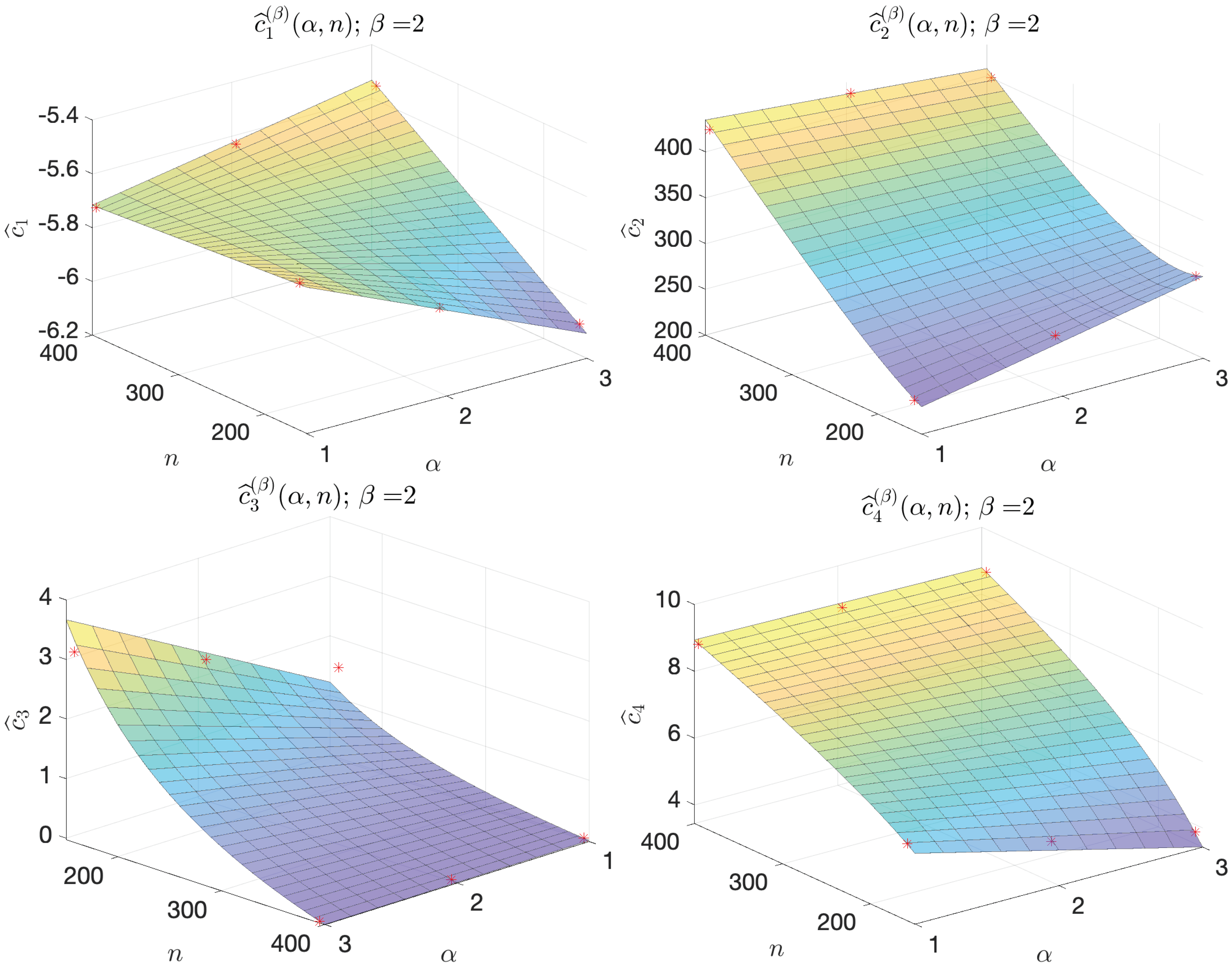
Thanks to Proposition 1, we can define a rule-of-thumb “UQ rule” for users who need to perform UQ on a DFN, with a number of fractures n in the order of magnitude around 158–395 generated by similar laws (Section 2.1.2) and who want to understand whether it is convenient to train an NN as a reduced model. This rule is based on the regular behavior characterizing the coefficients ${\widehat{c}}_1,\dots ,{\widehat{c}}_4$ of $\widehat{E}(\sigma ,\vartheta )$, varying the hyperparamenters $\alpha$ and n for each fixed $\beta$. Indeed, for each fixed $\beta$ and $i=1,\dots ,4$, we observe that the values of the coefficient ${\widehat{c}}_i$ with respect to $(\alpha ,n)$ are well-approximated by the function ${\widehat{c}}_i^{\left(\beta \right)}(\alpha ,n)$ defined in

Table 5. Parametric expressions of the functions ${\widehat{c}}_i^{\left(\beta \right)}(\alpha ,n)$ fitting the coefficients ${\widehat{c}}_1,\dots ,{\widehat{c}}_4$.

i	Function ${\widehat{\mathit{c}}}_{\mathit{i}}^{\left(\mathit{\beta }\right)}(\mathit{\alpha },\mathit{n})$
1	${\widehat{c}}_1=(d_1+d_{2}n)\alpha +(d_3+d_4\alpha )n+d_5$
2	${\widehat{c}}_2=(d_1+d_2/n)\alpha +d_{3}n+d_4$
3	${\widehat{c}}_3=(d_1+d_2/n)\alpha$
4	${\widehat{c}}_4=(d_1+d_2/n)\alpha +d_{3}n+d_4$

and

Table 6. Coefficient values for parametric expressions of the functions ${\widehat{c}}_i^{\left(\beta \right)}(\alpha ,n)$ fitting the coefficients ${\widehat{c}}_1,\dots ,{\widehat{c}}_4$.

i	$\mathit{\beta }$	${\mathit{d}}_1$	${\mathit{d}}_2$	${\mathit{d}}_3$	${\mathit{d}}_4$	${\mathit{d}}_5$
1	1	$-0.3002$	0.1372	$-0.0006$	$-0.1362$	$-5.467$
	2	$-0.417$	$-0.3173$	$-0.0015$	0.3185	$-5.201$
2	1	$-45.67$	$12750$	1.094	5.067	-
	2	$-39.07$	$10340$	0.9935	50.72
3	1	$-0.738$	291.5	-	-	-
	2	$-0.748$	295.5	-	-	-
4	1	0.38	$-139.8$	0.0121	3.698	-
	2	0.52	$-237.1$	0.0096	5.168	-

and illustrated in Figure 9 and Figure 10. The expression of the function ${\widehat{c}}_i^{\left(\beta \right)}$ was chosen by looking at the positions of the points $(\alpha ,n,{\widehat{c}}_i)$ in the space ${\mathbb{R}}^3$, for each $i=1,\dots ,4$ and each $\beta =1,2$; future analyses, involving more DFNs (i.e., more cases for n), may surely help find better-fitting functions to describe the behavior of the coefficients ${\widehat{c}}_i$.

Given the functions ${\widehat{c}}_1^{\left(\beta \right)}(\alpha ,n),\dots ,{\widehat{c}}_4^{\left(\beta \right)}(\alpha ,n)$, for each fixed $\beta =1,2$, we can define a function

$${\widehat{E}}_{\beta }(\sigma ,\vartheta ,\alpha ,n)=e^{\left({\widehat{c}}_1^{\left(\beta \right)}(\alpha ,n)+\frac{{\widehat{c}}_2^{\left(\beta \right)}(\alpha ,n)}{\vartheta }+{\widehat{c}}_3^{\left(\beta \right)}(\alpha ,n)\sigma +{\widehat{c}}_4^{\left(\beta \right)}(\alpha ,n){\sigma }^2\right)}$$

(23)

that returns estimates of the average errors $E_{\sigma }^{\vartheta }$ for any NN with architecture ${\mathcal{A}}_{\alpha }$ trained with respect to a number $\vartheta$ of simulations (and configuration $\beta$) to approximate the fluxes of a DFN with n fractures (see Section 2.1.2) and transmissivity variation characterized by $\sigma$. Then, the UQ rule exploits (23) and Proposition 1, and it is outlined by the following steps:

• Let $n\in \{159,\dots ,394\}\subseteq \mathbb{N}$ be the number of fractures of a given DFN with fixed geometry generated with respect to the characterization of Section 2.1.2, and let $\sigma$ be the parameter characterizing the standard deviation of the transmissivity distribution (see (1));
• For each $(\alpha ,\beta )\in \{1,2,3\}\times \{1,2\}$ and each arbitrary $\epsilon \in (e^{C_{\sigma }^{\left(\beta \right)}(\alpha ,n)},1)\subset \mathbb{R}$, following the results of Proposition 1, compute the values

  $${\vartheta }_{\epsilon }^{(\alpha ,\beta )}=-\frac{{\widehat{c}}_2^{\left(\beta \right)}}{(C_{\sigma }^{\left(\beta \right)}(\alpha ,n)-log\epsilon )},$$

  (24)

  where $C_{\sigma }^{\left(\beta \right)}(\alpha ,n):={\widehat{c}}_1^{\left(\beta \right)}(\alpha ,n)+{\widehat{c}}_3^{\left(\beta \right)}(\alpha ,n)\sigma +{\widehat{c}}_4^{\left(\beta \right)}(\alpha ,n)+{\sigma }^2$. Then, the values ${\vartheta }_{\epsilon }^{(\alpha ,\beta )}$ represent the estimates of the minimum number of simulations required by the NNs ${\mathcal{A}}_{\alpha }$, trained with respect to configuration $\beta$, in order to return an average error $E_{\sigma }^{\vartheta }$ less than or equal to $\epsilon$.

The reliability of the values ${\vartheta }_{\epsilon }^{(\alpha ,\beta )}$ depends strictly on the reliability of $\widehat{E}(\sigma ,\vartheta )$ representing the values $E_{\sigma }^{\vartheta }$ and on the reliability of the functions ${\widehat{c}}_i^{\left(\beta \right)}(\alpha ,n)$ representing the coefficients ${\widehat{c}}_i$. Therefore, we conclude this section by testing the efficiency of the UQ rule and, consequently, the reliability of the expressions chosen in this work for the functions $\widehat{E}(\sigma ,\vartheta ),{\widehat{c}}_1^{\left(\beta \right)}(\alpha ,n),\dots ,{\widehat{c}}_4^{\left(\beta \right)}(\alpha ,n)$.

We validate and test the UQ rule with respect to DFN202, a DFN with $n=202$ fracture ($m=14$ outflow fractures) and transmissivity distribution characterized by $\sigma =1/3$. We train an NN ${\mathcal{A}}_{\alpha }$ with configuration $\beta \in \{1,2\}$ on a number of simulations ${\vartheta }_{\mathrm{act}}$ equal to (24) rounded up to the nearest multiple of five for each $\epsilon \in \{0.01,0.02,0.03\}$ and each $\alpha \in \{1,2,3\}$. For the case $(\alpha ,\beta )=(3,1)$, we do not use a value $\epsilon =0.01$ but a value $\epsilon =0.011$ because $0.01$ is too close to the infimum error value $e^{C_{\sigma }^{\left(\beta \right)}(\alpha ,n)}=0.0099$ and, indeed, in this case, ${\vartheta }_{\epsilon }^{(\alpha ,\beta )}$ is approximately equal to $20,000$; since we do not have enough simulations available to test $\epsilon =0.01$, we adopt $\epsilon =0.011$.

The average errors obtained for the test on DFN202 are reported in

Table 7. Values returned by validation of the Uncertainty Quantification (UQ) rule on DFN202 ($n=202$, $\sigma =1/3$).

	$\mathit{\beta }=1$					$\mathit{\beta }=2$
$\mathit{\alpha }$	${\mathit{e}}^{{\mathit{C}}_{\mathit{\sigma }}^{\left(\mathit{\beta }\right)}(\mathit{\alpha },\mathit{n})}$	$\mathit{\epsilon }$	${\mathit{\vartheta }}_{\mathit{\epsilon }}^{(\mathit{\alpha },\mathit{\beta })}$	${\mathit{\vartheta }}_{\mathrm{act}}$	${\mathit{E}}_{\mathit{\sigma }}^{\mathit{\vartheta }}$	${\mathit{e}}^{{\mathit{C}}_{\mathit{\sigma }}^{\left(\mathit{\beta }\right)}(\mathit{\alpha },\mathit{n})}$	$\mathit{\epsilon }$	${\mathit{\vartheta }}_{\mathit{\epsilon }}^{(\mathit{\alpha },\mathit{\beta })}$	${\mathit{\vartheta }}_{\mathrm{act}}$	${\mathit{E}}_{\mathit{\sigma }}^{\mathit{\vartheta }}$
1	0.0081	0.01	1162.2	1165	0.0097	0.0090	0.01	2449.3	2450	0.0080
		0.02	269.68	270	0.0221		0.02	329.09	330	0.0208
		0.03	186.09	190	0.0250		0.03	218.47	220	0.0323
2	0.0089	0.01	2339.1	2340	0.0085	0.0090	0.01	2709.7	2710	0.0071
		0.02	324.17	325	0.0226		0.02	346.75	350	0.0215
		0.03	215.55	220	0.0249		0.03	229.62	230	0.0254
3	0.0099	0.011	2555.8	2560	0.0086	0.0091	0.01	3001.9	3005	0.0079
		0.02	393.75	395	0.0195		0.02	364.66	365	0.0197
		0.03	250.20	255	0.0250		0.03	240.88	245	0.0253

. For each $(\alpha ,\beta )$, we report the minimum error value $e^{C_{\sigma }^{\left(\beta \right)}(\alpha ,n)}$, the chosen target error $\epsilon >e^{C_{\sigma }^{\left(\beta \right)}(\alpha ,n)}$, the estimated minimum number of simulations ${\vartheta }_{\epsilon }^{(\alpha ,\beta )}$, the number of simulations ${\vartheta }_{\mathrm{act}}\sim {\vartheta }_{\epsilon }^{(\alpha ,\beta )}$ performed for the training of the NN, and the final average error $E_{\sigma }^{\vartheta }$ returned by the trained NN on a test set ${\mathcal{P}}_{\sigma }$ (with $|{\mathcal{P}}_{\sigma }|=3000$). In all the cases, with ${\vartheta }_{\mathrm{act}}\sim {\vartheta }_{\epsilon }^{(\alpha ,\beta )}$, the error $E_{\sigma }^{\vartheta }$ is very close to the target error $\epsilon$.

4. Discussion

Some examples concerning the use of deep learning models to speed up UQ analysis can be found in [33,34]. The use of DNNs as surrogate models for UQ is still a novel approach that requires deep investigations but is very promising. To the best of the authors’ knowledge, other than [35,36,37], there are no works in the literature that train DNNs to perform flux regression tasks on DFNs and, in particular, that use these NNs in the context of UQ as in [35]. While the results illustrated in [35] are very promising, the ones presented in Section 3 of this work concerns the use of NN reduced models as a practical possibility in the UQ framework for flow analyses of a subsurface network of fractures.

Let us assume that we deal with a natural fractured basin that can be described by a number of principal fractures in the order of $\{158,\dots ,395\}$ and probability distributions for fractures and hydrogeological properties as in Section 2.1.2, with a fixed value $\sigma \in [0.2,0.7]\subset \mathbb{R}$. The stochastic flow analysis can be very relevant for geothermal energy exploitation and for enhanced oil and gas exploitation. Flux investigations can also be relevant in risk assessment for geological storage of nuclear waste. The approach could be extended to different situations, for example, to provide a statistical analysis of the effects of different fracturing approaches [46,47,48].

Uncertainty in fractures and hydrogeological properties requires the generation of an ensemble of DFNs describing the principal flow properties of the basin, and consequently, a UQ analysis of the flow properties is required. The results presented in Section 3.3 can be useful for deciding if the training of a DNN is convenient with respect to a Monte Carlo approach or the use of a different surrogate flow model. Thanks to the results in Section 3.3, we have the possibility to fix an approximation tolerance $\epsilon >0$ such that an NN trained on $\sim {\vartheta }_{\epsilon }$ simulations fits the target tolerance.

Let us provide an example with DFN202, the validation DFN of Section 3.3 ($\sigma =1/3$). During a UQ analysis for this DFN, a standard approach may need thousands of simulations to obtain good estimations of the mean value and the standard deviation of the flux exiting from the DFN. Nevertheless, the UQ rule tells us that we can train an NN with approximately $2\%$ or $1\%$ average error with less than 300 simulations or approximately 1000 simulations, respectively (see Table 7, $(\alpha ,\beta )=(1,1)$ case). Then, once that has been trained, a NN can return virtually infinite reliable predictions (i.e., approximations) of the DFN exiting fluxes, varying the fracture transmissivities, in the order of seconds; therefore, we can estimate the exiting flux’s momentum using the NN predictions with a total cost of only the $\sim {\vartheta }_{\epsilon }$ DFN simulations used to train the NN. If we repeat the procedure for each geometry of DFN generated for the study, the advantages are significant.

A possible drawback of our method is that a UQ rule must be defined for the family of problems and NN architectures considered. Indeed, the UQ rule defined in Section 3.3 is tailored on the multi-task architecture described in Section 2.2.3, applied to the family of DFNs defined by the probability distributions in Section 2.1.2. Moreover, the UQ rule of this work can be considered reliable at most for DFNs with few hundreds of fractures. The analysis performed here can be extended to larger DFNs and can provide useful information to wider applications.

The approach presented here is not immediately extensible to the case of DFNs with a stochastic geometry (see [49]) due to the continuous change in inflow and outflow fractures. Nevertheless, a similar approach could be extended to the case of analysis of flows through the DFN that occurs between a fixed set of wells. In that case, the NN can provide flow through fixed wells varying the DFN geometry and the hydraulic properties of the fractures. In that case, we expect that the number of training simulations increases but the proposed approach could provide information correlating the target error tolerance with the variance in the stochastic distributions and the number of fractures.

5. Conclusions

With this work, we proposed an analysis for the characterization of a family of DNNs with multi-task architecture ${\mathcal{A}}_{\alpha }$ trained to predict the exiting fluxes of a DFN given the fracture transmissivities. The novelty of this analysis consists in characterizing these NNs, searching for rules that describe the performances, varying the available training data ($\vartheta$) and the standard deviation of the inputs ($\sigma$). The results of our study show interesting common behaviors for all the trained NNs, providing characterization of the average error with the functions $\widehat{E}(\sigma ,\vartheta )$ and ${\widehat{E}}_{\beta }(\sigma ,\vartheta ,\alpha ,n)$ (see (19) and (23)). This result is interesting, since it shows that common characterizing formulas for NN performances exist, despite the stochastic nature of the NN training processes; thanks to these regularities, we are able to define a “UQ rule” that returns an estimate of the minimum number of simulations required for training an NN with an average error less than or equal to an arbitrary value $\epsilon >e^{C_{\sigma }}$.

This estimate can be fruitfully exploited in real-world problems. Indeed, in the framework of UQ, it suggests whether it is convenient to train an NN as a reduced model and that a user can choose the best strategy between the use of an NN or direct simulations. In particular, the estimate returned by the UQ rule can be exploited in all “real-world” applications in which flow through a DFN with stochastic trasmissivities is recommended. The fields of interest could be oil and gas extraction, where flows through a fractured medium that occur between a fixed set of wells need to be analyzed and the possible effects of phenomena that can impact the fracture transmissivities (for example clogging) should be foreseen. Similar needs could occur in designing geothermal sites for which the performances strongly depend on the flow properties. Other application examples could be flow analysis for geological risk assessments of geological carbon dioxide or nuclear waste storage or water prevention close to other pollutant storage sites. The usage of NNs as reduced models for DFN flow simulations, optimizing the number of required numerical simulations for training through the UQ rule, can save precious time when computing an estimate of the risks and, therefore, deciding how to intervene when preventing or managing a calamity.

In general, we believe that many approaches for underground flow analysis through DFNs can be endowed with a tailored version of the method proposed in this paper; then, the method can speed up the simulation process, which is often slow and expensive, granting considerable advantages in many real-world geophysical applications.