Abstract
The objective of this study is to provide a comprehensive review and characterization of selected climate variability indices. While we discuss many major climate variability mechanisms, we focus on four principal modes of climate variability related to the dynamics of Earth’s oceans and their interactions with the atmosphere: the El Niño–Southern Oscillation (ENSO), North Atlantic Oscillation (NAO), Pacific Decadal Oscillation (PDO), and Atlantic Multi-decadal Oscillation (AMO). All these oscillation modes are of broad interest and considerable relevance, also in climate impact studies related to teleconnections, i.e., relationships between climate variations at distant locations. We try to decipher temporal patterns present in time series of different oscillation modes in the ocean–atmosphere system using exploratory analysis of the raw data, their structure, and properties, as well as illustrating the quasi-periodic behavior via wavelet analysis. With this contribution, we hope to help researchers in identifying and selecting data sources and climate variability indices that match their needs.
1. Introduction
Trend detection in time series illustrating climate change is a very common research topic. However, there are strong deviations of a climate-related variable from a gradual, long-term trend that can likely be explained by natural, internal climate variability. The availability of time series of indices representing different climate variability patterns makes it possible to undertake impact studies at various scales, from local to regional to continental to global.
The term climate variability generally describes variations in the climatic system. A part of the climate variability is strictly periodic. Another part is quasi-periodic and occurs in the form of distinct modes of climate patterns, but not in regular time intervals. Yet another part of variability does not appear to occur regularly, but rather at random times. The only climate driver with an annual global mean value gradually increasing over many decades is the atmospheric concentration of greenhouse gases, such as carbon dioxide (also methane and nitrous oxide). The uninterrupted series of the annual mean CO2 concentration at the Mauna Loa station (Hawaii, USA) is increasing regularly since records began in March 1958, while the seasonal variability within one year reflects the vegetation cycle in the Northern Hemisphere.
The objective of this study is to provide a guided tour of climate variability indices. The number of relevant contemporary data sources is substantial and keeps growing, so it becomes increasingly difficult to navigate in that realm. In this contribution, we provide a review of indices and their characterization, intending to help researchers in keeping pace with developments, in particular to ease the process of locating data sources and selecting variables that match their needs.
While we discuss many major climate variability mechanisms, we focus on four principal modes of climate variability, all of them related to the dynamics of the planet’s oceans and their interactions with the atmosphere: the El Niño–Southern Oscillation (ENSO), North Atlantic Oscillation (NAO), Pacific Decadal Oscillation (PDO), and Atlantic Multi-decadal Oscillation (AMO). All these modes are of considerable and broad interest, also in climate impact studies related to teleconnections, i.e., relationships between climate variations in places located far away from each other. For example, Kundzewicz et al. [1,2] analyzed links of indices of oscillation in the ocean–atmosphere system with abundance of water (intense precipitation, high river discharge, floods), while Kundzewicz et al. [3] studied links with global annual temperature and Norel et al. [4] examined relationships with river runoff using machine learning.
There is a superposition of periodic forcings of Earth’s climate, ranging from very high frequency to very low frequency. The obvious components are related to the eastward rotation of Planet Earth, with the period of 24 h, and to orbiting the sun, with the period of 365.256 days. Earth’s orbit is approximately an ellipse, whose center is close to the center of the sun. However, orbital parameters of Earth’s revolution, which can be regarded as Earth’s climate drivers, cyclically change with multi-millennial periodicity. Milanković [5] considered three cycles in orbital parameters of Earth’s revolution movement: orbital eccentricity with a period of 100,000 years, obliquity (axial tilt) with a period of 41,000 years, and precession with a period of 23,000 years. Changes in the geometry of the orbit of Planet Earth influence the amount of insolation. They have been found responsible for changes in the incoming solar energy received by the surface of the planet and allow us to interpret, among others, ice ages. However, due to co-occurrence of multiple interacting drivers, a periodicity of a climate driver may or may not show up as a cyclicity, or a quasi-cyclicity, in Earth’s climate.
The random components of the climate variability of Planet Earth are related to irregular, non-periodic climate drivers, such as volcanic eruptions or collisions with large extraterrestrial objects. A large asteroid, 10–15 km wide, is believed to have caused the extinction of dinosaurs 66M years ago [6]. This ancient collision may have produced a long winter due to global dispersal of dust and sulfates, blocking sunlight and resulting in a large temperature drop, leading to a multi-year halt of photosynthesis and breaking the food chain. Extinction of phytoplankton and plants led to dying out of all dependent organisms. The discovery of the Chicxulub Crater in the Yucatán Peninsula (Mexico) of 180 km diameter supports the Alvarez theory [7].
Volcanic eruptions are also climate drivers. The world’s most recent gigantic volcanic eruption, when the volcanic eruptivity index (VEI) [8] attained the value of eight and the volume of deposited volcanic material exceeded 1000 km3, was the so-called Oruanui eruption of the Taupo Volcano in New Zealand, some 26,500 years ago. Even stronger was the eruption of the Toba Supervolcano some 70,000 years ago. In historic times, eruption of the Tambora Volcano in April 1815 caused a year without summer, observed in much of the Northern Hemisphere in 1816 [9]. Three VEI-6 eruptions have been recorded since 1900: Santa Maria (1902), Novarupta (1912), and Mount Pinatubo (1991). The latter eruption was the largest stratospheric disturbance since the Krakatoa eruption in 1883 that clearly influenced the global climate, as did also the El Chichón eruption (VEI-5) in 1982, during which 7 million tons of sulfur dioxide were emitted to the stratosphere.
The present paper deals with selected quasi-periodic oscillations in Earth’s climate that can be seen as a combination of patterns. Among quasi-periodic modes of variability of climate or climate forcings are (i) quasi-periodic changes in solar activity (sunspot numbers) and (ii) oscillations in the ocean–atmosphere system. They are not perfectly periodic and have no sharp Fourier spectrum. Solar irradiance, illustrated by sunspot numbers whose principal periodicity is about 11 years (the so-called Schwabe cycle [10]), is a likely driver of climate variability.
In this study, we focus on ocean–atmosphere oscillations, which are a primary manifestation of Earth’s climate variability, driving climate impact variability. They consist of alternating occurrences of positive and negative anomalies of differences between values of meteorological variables, such as temperature or air pressure, in two specific reference locations. These spatially defined oscillations in the ocean–atmosphere system, related to heat and mass exchange between Earth’s atmosphere and the oceans, were found to affect the weather and climate and various climate impact variables on many spatial and temporal scales.
Many indices of climate variability modes have been introduced in the scientific literature in order to quantify oscillations in the atmosphere–ocean system. Among them are the El Niño–Southern Oscillation (ENSO); the Indian Ocean Dipole (IOD); a group of Northern Hemispheric teleconnection indices, such as the North Atlantic Oscillation (NAO), the Arctic Oscillation (AO), the North Pacific Oscillation (NPO)/North Pacific Index (NPI), the Northern Annular Mode (NAM), the Polar/Eurasia Pattern, the Siberian High-Intensity, the Scandinavia Pattern, the East Atlantic/Western Russia Pattern, the Pacific North American Pattern, and the Northern Hemispheric Circum-global Teleconnection; the Atlantic Multi-decadal Oscillation (AMO); the Pacific Decadal Oscillation (PDO) and the Pacific Interdecadal Oscillation (PIO); the Southern Annular Mode (SAM) and the Antarctic Oscillation (AAO); as well as monsoon indices (such as the Webster–Yang Monsoon Index, the South Asian Monsoon Index, and the East Asian–Western North Pacific Monsoon Index [11]). The present paper deals with a subset of the above oscillation modes. We discuss indices of ENSO, the NAO, the PDO, and the AMO that have been found important in studies of links between abundance of water (intense precipitation and floods) and climate variability as well as global annual temperature [1,3].
Some climate variability indices can be interrelated, i.e., one climate variability may force other modes of climate variability and modulate their properties. For instance, the PDO can modulate ENSO, possibly through atmospheric bridges and/or internal oceanic wave propagation (see the discussion in Kaplan [12]).
2. Materials and Methods
Studying properties and relations of indices of inter-annual and inter-decadal climate variability modes is contemporarily facilitated by the availability of long time series of records of climate oscillations available in the public domain. Table 1 contains the meta-data about the prominent large-scale climate variability modes considered in this paper (ENSO, NAO, PDO, AMO) and various indices used to define them. The list includes the modes and indices that have been defined relatively simply from raw or processed observations of a single surface climate variable and used by many authors. A well-designed climate index should simultaneously meet somewhat conflicting criteria of simplicity, relevance, and completeness, and it is these criteria that we followed in our selection of indices.

Table 1.
Information (meta-data) about the ocean–atmosphere oscillation indices considered in this paper. There are no missing values in datasets. All data are given as monthly values, except for the Oceanic Niño Index (ONI) NOAA (National Oceanic and Atmospheric Administration), where record values are 3-month running means. In contrast to other indices, with constant reference periods (mostly 1981–2010), the reference period for ONI NOAA is a centered 30-year base period updated every 5 years. Data used for analysis were retrieved on 7 July 2020.
Indices of climate variability are often defined as linear combinations of seasonally averaged anomalies of variables at meteorological stations chosen in the proximity of maximum and minimum values of the target pattern [12]. Changes in these indices are associated with large-scale changes in spatio-temporal climate fields. Since gridded fields of climate variables are available now, appropriate regional averages can be determined and used instead of station data.
We try to decipher temporal patterns present in time series of indices of climate variability using exploratory analysis of the raw data, their structure, and properties (dynamics, range, rate of change, temporal autocorrelation). To provide insight into temporal characteristics of the indices, in the sections that follow, we scrutinize them using autocorrelation and wavelet analysis. Wavelet analysis has become a useful tool for studying of non-stationary time series and modes of variability, with applications in Earth system science. Torrence and Compo [13] were pioneers in using wavelet analysis for an example of time series of the Niño 3 index of ENSO. They tackled the choice of a wavelet basis function, discussed edge effects due to finite-length time series, and demonstrated the relationship between the wavelet scale and the classical Fourier wavelength. In this paper, wavelet analysis was carried out using tools available in Python language libraries, following https://github.com/regeirk/pycwt, with brief documentation available at https://pycwt.readthedocs.io/en/latest/#. This also holds for wavelet-related illustrations presented in this paper and in the Supplementary Material. The Morlet wavelet basis was used in all analyses.
3. Indices of Inter-Annual and Inter-Decadal Climate Variability
3.1. El Niño–Southern Oscillation (ENSO)
3.1.1. Origins and characterization
The El Niño–Southern Oscillation (ENSO) mode of climate variability, associated with irregular, quasi-periodic variation of sea surface temperature (SST) and air pressure (AP) over the tropical Pacific Ocean, is likely the dominant, most powerful, demonstrably coupled inter-annual climate signal and the most important phenomenon in the interaction of the dynamics of the atmosphere and the ocean worldwide.
The phenomenon of ENSO has been known for more than a hundred years. Sir Gilbert Walker, a British mathematician who served in the British Colonial Service as Director General of the Meteorological Observatory in India, was a pioneer in postulating a connection between AP variability and Indian monsoon failure (see [14]). Nearly half a century later, Bjerknes [15] demonstrated a link between the AP oscillation (Southern Oscillation (SO)) and the SST oscillation. Major features of the combined ENSO phenomenon depend on large-scale spatial distributions of the oceanic component—SST and the accompanying atmospheric component, AP. There is a large-scale see-sawing pattern of SST change coupled with the mean sea level AP between the eastern and western sides of the tropical Pacific.
The so-called Walker circulation system results from a difference in the AP and SST over the western and eastern tropical Pacific Ocean. In a positive SO phase, there is a low-pressure system over the tropical western Pacific (e.g., Indonesia), being warm and wet, while a high-pressure system over the eastern Pacific brings cool and dry conditions. This creates a pressure gradient from east to west that causes surface air to move in that direction, while west-to-east winds higher in the atmosphere complete the Walker circulation. A Strong Walker circulation during a pronounced positive SO phase, so-called La Niña (alternative name El Viejo), causes upwelling of deep and cold seawater in the eastern Pacific, markedly cooling the sea surface. When the Walker circulation reverses (negative SO phase called El Niño), there is high air surface pressure in the tropical western Pacific and amplified seasonal ocean surface warming in the eastern equatorial Pacific and the Peruvian coast because of the absence of cold upwelling. Between the so-called warm phase, El Niño, and the cold phase, La Niña, there is a neutral phase.
ENSO has been shown to affect the global atmospheric circulation and mean global temperature, as well as, via teleconnections, weather extremes (droughts, heat waves, wildfires, tropical cyclones, wet spells, and floods) that exert impacts on agriculture, food security, and ecosystems in much of the world. In brief, ENSO has considerable socioeconomic impacts worldwide. As postulated by McPhaden et al. [16], ENSO is indeed “an integrating concept in Earth Science.” Occurrence of El Niño can result in precipitation anomalies, affecting agricultural production in many of the world’s regions. In some regions, occurrence of drier-than-average conditions (with higher drought risk) is likely, while in other regions, occurrence of wetter-than-average conditions (with higher flood risk) is likely (Figure 1).
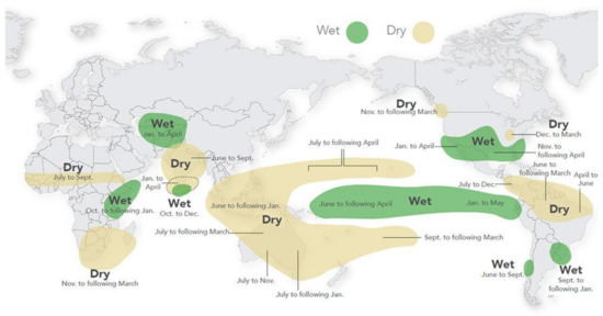
Figure 1.
Impacts of El Niño on rainfall. Source: http://www.fao.org/emergencies/crisis/elnino-lanina/en/ (accessed on 9 March 2021).
3.1.2. Indices
The ENSO mode has been characterized with several indices (cf. Table 1), introduced by various scientists and practitioners in order to meet their demands of illustrating specific aspects. One of most commonly used indices is the Niño 3.4 index [17], determined as SST anomalies averaged over the Niño 3.4 region, i.e., the area stretching from the 120° W to 170° W meridians astride the equator, 5° of latitude on either side (i.e., 5° N–5° S). The SST determination methodology is described in Huang et al. [18].
The Oceanic Niño Index (ONI) is a three-month running mean of SST anomalies in the Niño 3.4 region. According to the NOAA (National Oceanic and Atmospheric Administration) operational definitions, El Niño is characterized by a positive ONI of ≥+0.5 °C, while La Niña is characterized by a negative ONI of ≤−0.5 °C. To be classified as a full-blown El Niño or La Niña episode, these thresholds must be exceeded for a period of at least five consecutive overlapping three-month seasons. Figure 2 depicts a time series of El Niño and La Niña episodes, as defined above, for 1870–2019. For the source of the data, see Table 1. It is often claimed that occurrence of El Niño and La Niña episodes, as defined above and illustrated in Figure 2, affects the climate of large areas of the tropics and subtropics, changing the probability of occurrence of various climate anomalies in many regions of the world, via teleconnections. Therefore, we take a closer look into each of such episodes (Tables S1 and S2). There have been, respectively, 34 and 30 full-blown El Niño (Table S1) and La Niña (Table S2) episodes in 1870–2019.
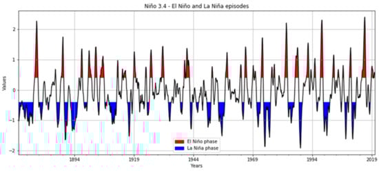
Figure 2.
Time series of El Niño and La Niña episodes, with at least five consecutive overlapping three-month seasons with Oceanic Niño Index (ONI) ≥ + 0.5 °C or ONI ≤ −0.5 °C, respectively. The basic time series corresponds to the Niño 3.4 record.
Tables S1 and S2 make it possible to evaluate the quasi-periodic properties of time series of El Niño and La Niña episodes. The value of average periods between the consecutive maxima of El Niño and between the consecutive minima of La Niña is equal to 53 and 61 months, respectively.
Huang et al. [19] discussed the ranking of the strongest El Niño and La Niña events while incorporating SST uncertainty. The strongest El Niño events were noted in 1982–1983, 1997–1998, and 2015–2016, while the strongest La Niña events were noted in 1955–1956, 1973–1974, and 1975–1976.
Figure 3 depicts the tendency of the quasi-periodicity of the Niño 3.4 index to decrease (i.e., this stage of the ENSO cycle becomes, on average, more frequent). In contrast, Figure 4 shows that the quasi-periodicity of La Niña has been increasing (i.e., this stage of the ENSO cycle becomes, on average, less frequent).
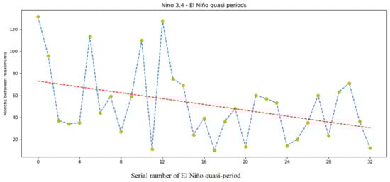
Figure 3.
Illustration of quasi-periodicity (time between consecutive maxima of El Niño episodes), based on Table S1. Numbers of episodes follow from this table. In this and following plots of quasi-periodicity, a regression line is added in red.
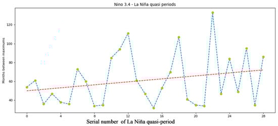
Figure 4.
Illustration of quasi-periodicity (time between consecutive minima of La Niña episodes), based on Table S2. Numbers of episodes follow from this table.
Novel insight into the quasi-periodic behavior of the Niño 3.4 index can be gained by wavelet analysis (Figure 5). Figure 5a presents a wavelet power spectrum of this time series. Periods (corresponding to frequencies) occupy the vertical axis, while time is presented horizontally. Bright colors indicate the strong response of the wavelet transform for a particular time point and a particular frequency. Darker colors mean low contribution of a frequency at a given time point. The red contour shows the areas of the spectrum with statistically significant peaks (with a 95% confidence level) when compared to the background, defined as a red noise process, as in Torrence and Compo [13]. The red noise is modeled as a Markov process in which every observation depends on its predecessor and some noise. In our analysis, the parameter that defines the strength of this dependency is set to lag-1 autocorrelation coefficient for the normalized time series. The cross-hatched area marks the invalid region where edge effects influence the results from wavelet transform, resulting from the fact that the time series is padded with zeros on both ends (beyond the time range shown in the figure). This region is wider for longer periods, because low frequencies require wider wavelets and thus longer padding sequences. The valid area of the spectrum is called the cone of influence, even though it might not look like a cone; however, note the logarithmic scale of the vertical axis.
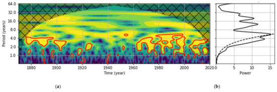
Figure 5.
Results of wavelet analysis of the Niño 3.4 index, illustrating the quasi-periodic behavior: (a) wavelet power spectrum and (b) global wavelet spectrum.
Figure 5b presents the global wavelet spectrum (averaged over time). The dotted line shows the 95% confidence level. The global wavelet spectrum is similar to the Fourier spectrum and is characterized by a strong response for the frequencies from 2.5 to 7 years. The maximum of the global wavelet spectrum corresponds to a period of slightly over 5 years. We can observe greater periodicity since 1960, and this characteristic seems to be present nowadays.
Figure 6 illustrates the autocorrelogram of the Niño 3.4 index. The graph corroborates observations of wavelet analysis, suggesting quite clearly that this index is not strictly periodic: correlation coefficients become quickly insignificant with the growing shift (lag).
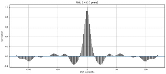
Figure 6.
The autocorrelogram of the Niño 3.4 index.
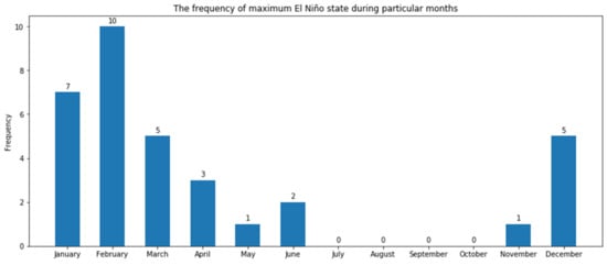
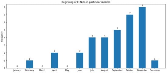
The name El Niño (boy child in Spanish) originates from the fact that Peruvian fishermen noted that in some years, the water of the tropical Pacific and Ecuadorian coast of South America is warmer than normal, adversely affecting fish catch. This behavior was often observed around Christmas, so the Catholic population associated the phenomenon with the new born Christ-child. In Figure 7 and Figure 8, we examine how the name fares with respect to reality, for Niño 3.4. Indeed, the maximum value of an anomaly during an El Niño episode often occurs in December (Figure 7). However, the beginning of El Niño can occur in many different months (Figure 8).
Once a month, NOAA provides updates on the ENSO evolution status (using ONI) https://www.cpc.ncep.noaa.gov/products/analysis_monitoring/lanina/enso_evolution-status-fcsts-web.pdf.
Among other indices related to ENSO are SST anomalies averaged over different areas, such as Niño 1 + 2 (0–10° S, 80° W–90° W), Niño 3 (5° N–5° S, 90° W–150° W), and Niño 4 (5° N–5° S, 150° E–160° W); see [17,20]. The Trans-Niño Index (TNI), which is defined as the difference in normalized SST anomalies between the Niño 1+2 and Niño 4 regions, is classified as Central Pacific El Niño or El Niño Modoki [21].
Figure S1 illustrates the values attained by various Niño indices: Niño 3.4, Niño 4, Niño 1 + 2, Niño 3, ONI, the El Niño Modoki index (EMI), and Equatorial SOI Indonesia.
There is a range of ENSO indices based on the differences in standard mean sea level pressure (MSLP) anomalies. The Southern Oscillation Index (SOI) and Troup SOI express fluctuations in air pressure between the western and eastern tropical Pacific, calculated based on the differences in air pressure anomalies between Tahiti and Darwin, Australia. Equatorial SOI expresses the difference of MSLP anomalies for the eastern Pacific (80° W–130° W) minus the western Pacific (90° E–140° E) in the equatorial zone (5° N–5° S).
Figure S2 illustrates the values of various SOI indices, except for Equatorial SOI Indonesia.
It should be noted that Equatorial SOI Indonesia is presented in Figure S1, together with Niño indices, rather than in Figure S2, where a group of SOI indices is presented. The reason is that the series of Equatorial SOI Indonesia better fits Niño indices than SOI indices.
It can be seen that Niño indices (Figure S1) are basically in counter-phase with SOI indices (Figure S2), i.e., the positive episodes of Niño indices correspond to negative episodes of SOI indices, and the other way round.
While we consider the maximum of the Niño 3.4 index, being commonly applied now as a measure of ENSO maturity (Figure 2, Figure 7, and Figure 8), we are aware that some authors [22] select the minimum of SOI that lends itself well to such studies. Pinault [22] filtered the SOI signal and selected 36 most significant events in 1867–2013, finding the average period of about four years. The Fourier spectrum had a peak centered at about 4 years and a broad peak extending beyond 6.5 years. A diagram of return period vs. amplitude [22] showed that the large 1982/1983 event (amplitude of 3.81) had a return interval of 148 years. Pinault [22] interpreted the dynamics of the tropical Pacific by invoking coupled oscillators and studied ENSO events [23] in the context of quadrennial quasi-stationary waves, examining their time lag, defined relative to the central value of successive intervals of a four-year length.
In the Supplementary Material, we provide complementary graphic material related to time series and quasi-periodic behavior (via wavelet analysis) of ENSO indices (Niño and SOI type) that are not included in the main text. Figures S3–S5 present time series of Niño indices; Figures S6–S11 present time series of SOI indices; Figure S12, the EMI; and Figure S13, the ONI. Figures S14–S16, analogously to Figures S3–S5, illustrate the quasi-periodic behavior of Niño indices via wavelet analysis, while Figures S17–S22, complementary to Figures S6–S11, illustrate the quasi-periodic behavior of SOI indices via wavelet analysis. Figure S23 presents the quasi-periodic behavior of the EMI and Figure S24 of the ONI.
Figure 9 illustrates the location of areas for which different ENSO indices are defined. Figure 10 shows the scale-averaged wavelet powers of the indices in the ENSO group, where each data point is the average, over all periods, of the wavelet spectrum at a given time point. The calculated value can be interpreted as a simple measure of periodicity. The year 1997 has the strongest observed response. However, it is not the case for all indices. For the EMI, it was the year 2009, and for the SOI from CRU, it was 1877. These two are the indices that feature the most and the least recent peak in periodicity. On the other hand, 1920–1960 is the range of low periodicity. However, that does not mean that the indices themselves had low amplitude in that period of time; rather than that, they were less periodic and more volatile.
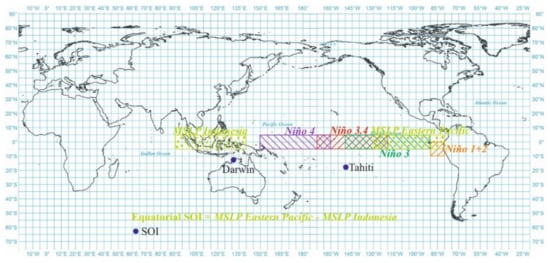
Figure 9.
Location of areas for which different ENSO indices are defined.
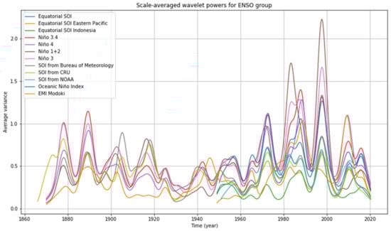
Figure 10.
Scale-averaged wavelet powers of indices in ENSO-related indices. Note various intervals of data availability as per Table 1.
3.2. North Atlantic Oscillation (NAO)
It was also Sir Gilbert Walker [14] who noticed quasi-periodic climate variability in the North Atlantic, later baptized as the North Atlantic Oscillation (NAO). The teleconnection pattern known as the NAO is characterized by a dipole in the sea level pressure field with one anomaly center over the Arctic and another anomaly center, of opposite sign, across the mid-latitude sector of the North Atlantic Ocean.
The term NAO is operationalized as cyclic air pressure changes in the Icelandic Low and Azores High as well as cyclic displacements of the center of the Azores High. If the (seasonal or monthly) value of the NAO index is positive, then there is a stronger contrast in air pressure between the Icelandic Low and the Azores High, i.e., the pressure value in the Azores Region is higher than the long-term average, while the pressure in the Icelandic Region is lower than the long-term average. Several experts have proposed indices to measure the strength of the NAO, related to air pressure at various observation stations, where long-term air pressure records are available. Three notable examples are the Hurrell index, the difference of air pressure between Lisbon (Portugal) and Stykkishólmur (Iceland); the Rogers index, between Ponta Delgada (Azores) and Akureyri (Iceland); and the Jones index, between Gibraltar and Stykkishólmur. Figure 11 illustrates the location of stations for which different NAO indices are defined.
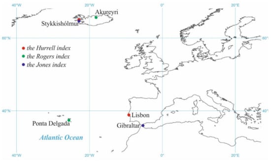
Figure 11.
Location of stations for which different NAO indices are defined.
More detailed information on the concept and studies of the NAO can be found in Wanner et al. [24].
The NAO mode of natural variability influences the continents adjacent to North Atlantic–Europe and North America. During a positive phase of the NAO index, the Atlantic storm track strengthens and moves northward. European winters are warm and wet then, while in Greenland and northeastern Canada, winters are cold and dry. During a negative phase of the NAO index, the storm track is weaker and more eastward in direction, resulting in wetter winters in southern Europe and the Mediterranean and a colder northern Europe [12].
In terms of sensible climate, the NAO is associated with a pattern in temperature and precipitation between northern Europe and Greenland. Jones et al. [25] compared various instrumental NAO indices and assessed the strengths and variability of their relationships with wintertime temperature and precipitation patterns over Europe. They showed that the influence of the NAO has varied over the past 150–200 years, being strongest recently and during the late 19th and early 20th centuries and weaker at other times.
Feldstein [26] studied the dynamics of the growth and decay of the NAO teleconnection pattern. He found the positive NAO phase to develop after anomalous wavetrain propagation across the North Pacific to the east coast of North America, while the negative NAO phase appeared to develop in situ.
There are attempts to extend the NAO record by using proxy-based reconstruction of the local NAO impact and external forcings, such as volcanic eruptions and solar activity, affecting NAO variability (e.g. [27]). Luterbacher et al. [28] used instrumental station pressure, temperature, and precipitation measurements and proxy data to statistically reconstruct monthly time series of the NAO and Eurasian circulation indices back to 1675. Figure 12 depicts an ensemble of time series of NAO indices (NAO from CRU, NAO Hurrell index, NAO PC-based Hurrell index, NAO index, and NAO from NOAA) in 1950–2019. Figures S25–S28 in the Supplementary Material present individual time series of NAO indices, while Figures S29–S31, analogously to Figures S25–S28, illustrate quasi-periodic behavior of various NAO indices via wavelet analysis.
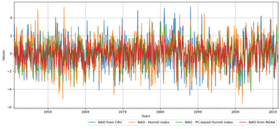
Figure 12.
Time series of NAO indices (NAO from CRU, NAO Hurrell index, NAO PC-based Hurrell index, and NAO from NOAA) in 1950–2019.
In Section 3.1.2, Figure 2 that illustrates the time series of full-blown El Niño and La Niña episodes, was used to aid the interpretation of Figure 3 and Figure 4. Now, we use a similar approach to mark the episodes of strong positive and strong negative phases in the NAO. To do so, we experimented with the parametrization of the definitions of strong positive/negative phases, i.e., the threshold (0.3, 0.4), the size of the moving window of consecutive months (3, 4, or 5 months), and the duration of excursion (threshold crossing), being 4, 5, or 6 months. Figure 13 illustrates the identification of strong positive and strong negative phases of the NAO, analogous to full-blown El Niño and La Niña episodes, for the following selection of parameters: threshold = 0.3; window size (running mean) = 5 months; and duration of excursion = 5 months.
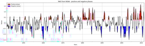
Figure 13.
Time series of episodes of strong positive and strong negative phases of the NAO.
Figure 14 and Figure 15 depict the tendency of the quasi-periodicity of both positive and negative phases of the NAO (see Figure 13 and Tables S3 and S4) to decrease.
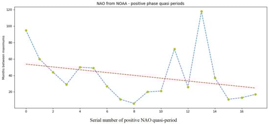
Figure 14.
Illustration of quasi-periodicity (time between consecutive maxima of NAO episodes), based on Table S3. Numbers of episodes follow from this table.
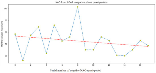
Figure 15.
Illustration of quasi-periodicity (time between consecutive minima of NAO episodes), based on Table S4. Numbers of episodes follow from this table.
Additional insights into the quasi-periodic behavior of the NAO index can be gained by wavelet analysis (Figure 16). The whole NAO family is quite volatile, which should not come as a surprise as the NAO is derived from sea level pressure, which is changing much faster than the sea level temperature. This is the main cause for why many methods struggle with these indices. Still, wavelet analysis can provide some useful information. For instance, in Figure 16, around the years 1970 and 2011, one can observe regions in the joint time–frequency space that are characterized with activity greater than the baseline noise. In other words, wavelet analysis managed to identify a structure around those time periods, which invites further investigation.
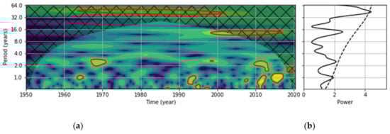
Figure 16.
Results of wavelet analysis of the NAO index, illustrating the quasi-periodic behavior: (a) wavelet power spectrum and (b) global wavelet spectrum.
Cohen and Barlow [29] examined relations between NAO, the closely related hemispheric-wide pattern of variability referred to as the Arctic Oscillation (AO) or annular mode, and the global warming. The NAO is regarded as a regional manifestation of the AO. The AO index is typically determined in a different way than the NAO index, which was derived from station data. Thompson and Wallace [30] used the principal component of the time series and spatial loading pattern associated with the first empirical orthogonal function (EOF) of the NH (Northern Hemisphere) sea level pressure, poleward of 20°N. They showed that the temperature pattern associated with the AO closely resembles that associated with the NAO. Since the NAO and AO were in a positive trend for much of the 1970s and 1980s, with historic high values in the early 1990s, they may have contributed significantly to the warming signal in the Northern Hemisphere and globally. Possibly, also such factors as North Atlantic SSTs, Indo–Pacific warm pool SSTs, stratospheric circulation, and the Eurasian snow cover are related to the NAO and AO. It has been argued that the observed positive trend in the AO index over the past three decades of the 20th century could significantly contribute to the observed warming trend over Eurasia and North America.
Ambaum and Hoskins [31] examined relationships between surface pressure variations associated with the NAO, tropopause height, and the strength of the stratospheric vortex. They found that an increase in the NAO index leads to a stronger stratospheric vortex as a result of increased equatorward refraction of upward-propagating Rossby waves. At the tropopause level, the effects of the enhanced NAO index and stratospheric polar vortex are opposite, resulting in a lower tropopause over Iceland and a higher tropopause over the Arctic. Ambaum and Hoskins [31] quantified the connection between stratospheric potential vorticity anomalies and the troposphere. Anomalies in the stratospheric vortex strength are associated with anomalies in the Atlantic region that are very similar to the signatures of the NAO. Hence, the stratosphere can be regarded as an integrator of the NAO index.
3.3. Pacific Decadal Oscillation (PDO)
The Pacific (inter) Decadal Oscillation (PDO) is another manifestation of the variability in the ocean–atmosphere system. It is a decadal-scale temperature oscillation pattern of the surface waters of the Pacific Ocean, occasionally referred to, rather colloquially, as a long-lived ENSO-like Pacific climate oscillation pattern. The PDO is a leading mode of multi-decadal variability in SSTs in the extratropical North Pacific. It is centered over the Pacific Ocean and North America, where PDO variations are most energetic in the boreal winter and spring. Tracking PDO variations is typically done with the help of indices constructed from observed Pacific SST and sea level pressure (SLP) patterns. The principal PDO index is defined as the leading empirical orthogonal function (EOF) of the North Pacific (above 20° N) SST anomalies [32].
The causes of decadal variability of SST in the North Pacific have long been a subject of intense debate. Schneider and Cornuelle [33] stipulated that the PDO pattern is qualitatively consistent with the atmospheric forcing associated with fluctuations of the position and strength of the Aleutian Low. They suggested that in the central North Pacific, a deepened Aleutian Low decreases the SST “by advection of cool and dry air from the north, by increases of westerly winds and ocean-to-atmosphere turbulent heat fluxes, and by strengthened equatorward advection of temperature,” while in the eastern regions, a deepened Aleutian Low “enhances poleward winds and leads to warm anomalies of surface temperature.” There is a horseshoe-like spatial pattern of the PDO, with SST anomalies in the central North Pacific surrounded by anomalies of the opposite sign in the Alaska gyre, off California, and toward the Tropics [33].
During the warm (positive) phase of the PDO, the SSTs are low in the central North Pacific, while there are anomalously high SSTs in the Eastern Pacific along the west coast of the Americas [32]. During the cool (negative) phase of the PDO, the opposite pattern prevails. Temperature anomalies (departures from average) in the Eastern Pacific (off the west coast of North America) have an opposite sign to those in the Western Pacific; therefore, from the global viewpoint, there could be some compensation effect, and the impact of the PDO on the global temperature is probably relatively small [34]. PDO anomalies extend through the depth of the troposphere and are well expressed as persistence in the Pacific North America (PNA) teleconnection pattern.
The PDO may be interpreted as a blend of two largely independent modes having distinct spatial and temporal characteristics of the North Pacific SST variability [35]. A notable feature of the indices is their tendency for year-to year persistence. The warm (positive) or cool (negative) index values tend to prevail for 20–30-year periods. Mantua [32] noted that PDO fluctuations were most energetic in two general quasi-periodicities, one from 15 to 25 years and the other from 50 to 70 years. D’Orgeville and Peltier [36] identified the 20-year quasi-periodic oscillation as a phase-locked signal at the eastern boundary of the Pacific basin, which could be interpreted as the signature of an ocean basin mode.
Figure 17 illustrates the time series of the PDO index. There were two full PDO quasi-cycles in the 20th century. Figure 18 presents the results of its wavelet analysis, which provides (arguably limited) evidence for its quasi-periodic behavior.
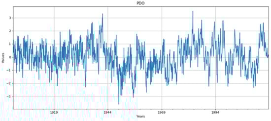
Figure 17.
Time series of the PDO index.
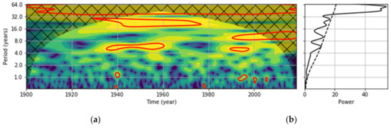
Figure 18.
Results of wavelet analysis of the PDO index, illustrating the quasi-periodic behavior: (a) wavelet power spectrum and (b) global wavelet spectrum.
There are considerable climatic and environmental impacts of PDO phases in the Pacific and over North America that have attracted considerable attention. Actually, the very term Pacific Decadal Oscillation (PDO) was proposed by an impact (fisheries) scientist, Steven Hare, who studied connections between Alaska salmon production cycles and Pacific climate [37]. Links were found between Northeast Pacific marine ecosystems and the PDO. Warm PDO episodes have favored high salmon production in Alaska and low salmon production off the west coast of California, Oregon, and Washington states, while cool PDO eras have favored low salmon production in Alaska and relatively high salmon production in California, Oregon, and Washington [35,37]. The warm and cool PDO episodes were found to be related to the Pacific and North American anomalies of ocean and temperatures, precipitation, snow pack, and streamflow [32]. For instance, for a warm phase of the PDO, October–March precipitation in the southern U.S. and northern Mexico is above average, while it is below average in northwestern North America and the Great Lakes. In a cool phase of the PDO, it is the other way round. In western North America, positive phases of the PDO are associated with climatic conditions somewhat similar to El Niño, although weaker in expression. Kim et al. [38] showed how the PDO drives the characteristics of sea ice extent in the Pacific Arctic sector.
The PDO notion is similar to the Interdecadal Pacific Oscillation (IPO). There are several indices expressing the IPO. Recently, the IPO Tripole Index (TPI), associated with a distinct tripole pattern of SST anomalies, based on the difference between the SST anomalies averaged over the Central Equatorial Pacific, the Northwest Pacific, and the Southwest Pacific, is commonly used [39].
3.4. Atlantic Meridional Oscillation, a.k.a. Atlantic Multi-Decadal Oscillation (AMO)
Meridional circulation of the Atlantic Ocean (the Atlantic Meridional Oscillation, a.k.a. the Atlantic Multi-decadal Oscillation (AMO)) can be described as a coherent pattern of oscillatory changes in the North Atlantic SST with a period of about 60–90 years, marking internal climatic variability. It is indexed by the average SST with the long-term trend removed [40,41]. Mann et al. [42] examined five AMO-related indices. Traditionally, indices of the AMO have been based on average annual SST anomalies in the North Atlantic. For example, the AMO index may be defined as the first empirical orthogonal function (EOF) of SST anomalies in the North Atlantic region, extending between 20° N–65° N and 100° W–0° E. Temperature anomalies in the North Atlantic have an opposite sign to those in the South Atlantic. The nature and origin of the AMO is uncertain, and it remains unknown whether it represents a persistent, quasi-periodic driver in the climate system, or merely a transient feature. A deterministic mechanism relying on the atmosphere–ocean–sea ice interactions for the AMO was proposed by Dima and Lohmann [43].
Figure 19 presents time series of the AMO index (raw values and 15-year moving average), comprising more than two periods of oscillation, while Figure 20 shows the Fourier spectrum of the AMO index, and Figure 21 illustrates results of the wavelet analysis of the AMO index. The AMO has strong low-frequency oscillations. For higher frequencies, there are hardly any regions in the spectrogram that stand out significantly from the background noise, so there is little or no evidence of a periodic or quasi-periodic behavior at a shorter timescale.
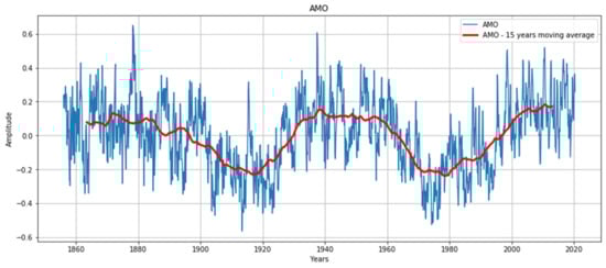
Figure 19.
Time series of the AMO index (raw values and 15-year moving average).
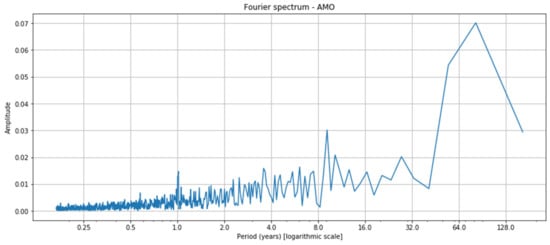
Figure 20.
Fourier spectrum of the AMO index.
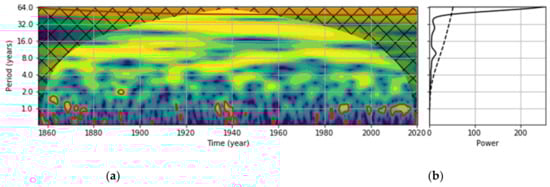
Figure 21.
Results of wavelet analysis of the AMO index, illustrating the quasi-periodic behavior: (a) wavelet power spectrum and (b) global wavelet spectrum.
Pinault [44] hypothesized that the AMO may be related to the resonance of the 64-year average period gyral Rossby waves (GRWs). He also noted that the AMO is almost in phase with the sunspot numbers.
Another notion of internal Atlantic circulation is the Atlantic Meridional Overturning Circulation (AMOC), referring to coupled ocean–atmosphere processes [42,45]. It is also referred to as thermohaline circulation, that is, ocean circulation driven by temperature and salinity changes. The AMOC is the ocean current consisting of a warmer northward flow near the surface of the Atlantic Ocean and a colder deep southward return flow. The physical mechanism of the overturning circulation is that heat loss to the atmosphere at high latitudes in the North Atlantic renders the northward-flowing surface waters denser and causes them to sink to considerable depths, where they constitute the deep southward return flow of the overturning circulation. In their review paper on the Atlantic Meridional Overturning Circulation (AMOC), Srokosz et al. [45] discuss the links between the AMO and the AMOC. Such links of changes in the AMO to decadal variability in atmospheric blocking in winter, with possible feedback to the AMOC, could be used to forecast the future behavior of the AMOC.
A weakening of the AMOCwould have huge impacts, cooling the North Atlantic and adjacent land regions, e.g., Scandinavia, or reducing the rate of temperature increase associated with global warming. A weakened AMOC is typically accompanied by a slight warming of the Southern Hemisphere.
The AMOC is a great ocean conveyor belt that—as the history of Earth’s climate demonstrates—can be deconstructed [46]. Rahmstorf [47] identified warm, off, and cold modes of AMOC operation. The first corresponds to the current AMOC configuration, the second to no northward warm water flow at the surface, and the third to the situation in which the AMOC exists but the surface warm waters do not reach as far north as the Nordic Seas and rather sink and form a shallower return flow south of Iceland. A harbinger of possible future (melt of Greenland ice and massive freshwater inflow to the northern ocean) was the so-called 8.2-kyr event, when large outbursts of fresh water, from ice-dammed lakes in North America, entered the North Atlantic and disrupted the AMOC, causing its shutdown [48].
Future changes in the AMOC could therefore have significant climatic impacts, possibly affecting the North Atlantic sink for CO2, the position of the intertropical convergence zone, the Atlantic storm track, rainfall, and marine ecosystems.
3.5. Links between Various Modes
In addition to discussing individual modes and indices in separation, it is worth looking for links between them in the hope to capture higher-level dependencies and dynamics and so arrive at better explanations of the global climate system.
Various indices of ENSO are clearly similar, as illustrated in Supplementary Materials. There exists a phenomenon on the Indian Ocean, bearing some analogy and links to ENSO. It is the Indian Ocean Dipole (IOD), being an irregular oscillation of the SST, in which the western part of the ocean becomes alternately warmer or cooler than the eastern part. During the positive stage of the dipole, warming is observed in the western part, inducing a likely increase in East African rainfall and a higher-than-normal Indian monsoon, and cooling in the eastern part, inducing likely drought in Australia and Indonesia. When the dipole is negative, conditions are reversed, with warm water and an increase in precipitation in the eastern Indian Ocean and cooler and drier conditions in the western Indian Ocean. As hypothesized by Pinault [49], the resonant forcing of long ocean waves in the tropical Indian Ocean lends itself well to explain the IOD. There are possible links with the far western Pacific, belonging to the ENSO domain.
Since the PDO is colloquially called a long-lived ENSO-like Pacific climate oscillation pattern, it is interesting to examine links between the PDO and ENSO. Mantua [32] noted three main aspects distinguishing the PDO from ENSO:
- (i)
- The timescale: During the 20th century, PDO events persisted for 20–30 years, while typical ENSO events persisted for only 6–18 months.
- (ii)
- The essential climatic fingerprints of the PDO were most visible in the North Pacific/North American sector and secondary signatures existed in the tropics, while for ENSO, the opposite is true.
- (iii)
- Causes for the PDO are not well understood, while mechanisms driving ENSO are relatively well known.
Gershunov and Barnett [50] demonstrated that the PDO modulates climatic teleconnections between North American climate and the equatorial Pacific during the warm and the cool ENSO (respectively, El Niño and La Niña) phase episodes.
Mac Donald and Case [51] noted that in western North America, positive phases of the PDO are associated with climatic conditions similar to El Niño, although weaker in expression. These conditions include decreased winter precipitation, snowpack and streamflow in the northwest, and higher precipitation in the southwest. Conditions reverse during negative PDO phases.
Schneider and Cornuelle [33] demonstrated that the PDO index can be reconstructed as a response to changes in the North Pacific atmosphere (the Aleutian Low) resulting from its intrinsic variability, remote forcing by ENSO and other processes, and ocean wave processes in the so-called Kuroshio–Oyashio Extension, associated with the adjustment of the North Pacific Ocean by Rossby waves. The relative importance of these forcing processes for the PDO is frequency dependent, and the relative roles of forcing are likely to be site dependent. Noting that correlation is not causation, and statistical relations can only be disproved, and not proved, Schneider and Cornuelle [33] presented physical arguments for the hypothesized influences.
Newman et al. [52] found that variability of the PDO, on both inter-annual and decadal timescales, can be mimicked by modeling them as the sum of direct forcing by ENSO, the re-emergence of North Pacific SST anomalies in subsequent winters, and white-noise atmospheric forcing. They postulated that weak simultaneous correlation between ENSO and the PDO may be misleading, because anomalous tropical convection induced by ENSO influences global atmospheric circulation and hence alters surface fluxes over the North Pacific, forcing SST anomalies that peak a few months after the ENSO maximum in tropical east Pacific SSTs, in the form of atmospheric bridge. Newman et al. [52] argue that the PDO is dependent upon ENSO on all timescales, and they offer extensive discussion of seasonal behavior mechanisms.
Mantua [32] noted that combining PDO and ENSO information may enhance the quality of empirical North American climate forecasts. This is so because empirical studies suggest that ENSO’s influences on North American climate are strongly dependent on the phase of the PDO, and the canonical patterns of North American climate anomalies are most likely to occur if ENSO and PDO anomalies are in phase, that is, the warm PDO coincides with the warm ENSO phase (El Niño) and the cool PDO coincides with the cool ENSO phase (La Niña).
Under such circumstances, a cross-correlation analysis lends itself as a potentially promising tool, allowing us to obtain significant results for the PDO and ENSO. Figure 22 presents the cross-correlation between the PDO and Niño 3.4. We can state that these series have partly related characteristics: they rise and fall synchronously, as evidenced by the relatively high correlation coefficient of roughly 0.41 for the time shift of 2–3 months. Overall, the cross-correlation of these two time series achieves statistically significant values for lags close to zero. While both indices follow a similar shape, the PDO seems to involve an additional periodic component.
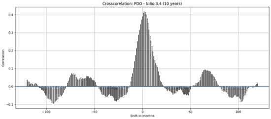
Figure 22.
Cross-correlation between the PDO and Niño 3.4.
There exist large-scale oceanic patterns of SST variability with multi-decadal timescales in both Northern Hemisphere oceans—the Pacific and the Atlantic. These patterns involve coupled ocean–atmosphere oscillation mechanisms. In Section 3.3 of this paper, we review the Pacific Decadal Oscillation, and in Section 3.4, we review the Atlantic Multi-decadal Oscillation. Here, we present the findings on relationships between the PDO and the AMO, drawing from d’Orgeville and Peltier [36] as well as Wu et al. [53].
D’Orgeville and Peltier [36] noted that because of the shortness of the observed SST reconstructions (130 years) compared to the multi-decadal timescale of 60 years, from a statistical point of view, there is a clear need for simulations that are able to reproduce the multi-decadal variability. Preliminary results obtained via statistical equilibrium simulations with the help of Atmosphere-Ocean Global Circulation Models (AOGCMs) demonstrate that a common multi-decadal mode of variability between the Pacific and Atlantic basins does indeed exist.
Wu et al. [53] studied the relationship between the dominant patterns of SST variability in the North Pacific and the North Atlantic. They hypothesized that the atmospheric anomalies over the North Pacific can propagate across North America in the form of stationary Rossby wavetrains and finally trigger atmospheric variation over the North Atlantic, possibly affecting the North Atlantic Oscillation. Hence, the North Pacific SST anomalies may lead to the North Atlantic SST anomalies through their modulation of the atmospheric circulation. Likewise, the North Atlantic SST anomalies can also affect the North Pacific SST through their modulation of mid-latitude storm tracks. Hence, the slowing down of the AMOC can affect the North Pacific SST through the Arctic Ocean and tropical oceans.
Wu et al. [53] stipulated that the AMO can exert a profound impact on the Northern Hemisphere, while the possible physical processes involved in the impact of the AMO on the PDO can be through three possible paths: the mid-latitude atmosphere, the Arctic Ocean, and tropical oceans.
Both d’Orgeville and Peltier [36] as well as Wu et al. [53] reported a significant lagged correlation between the PDO and the AMO, albeit their results are different. D’Orgeville and Peltier [36] demonstrated that the 60-year component of the PDO is strongly time-lag-correlated with the AMO. They showed the AMO to lead the PDO by about 13 years or to lag the PDO by 17 years, suggesting that the AMO and the 60-year component of the PDO can be signatures of the same oscillation cycle. In contrast, Wu et al. [53] found significant lagged correlation when the PDO leads the AMO by 1 year and the AMO leads the PDO by 11–12 years. Their analysis suggests that the correlation may arise from the ENSO forcing and the interaction between the Atlantic and Pacific Oceans through the overlying atmosphere. Although the correlation between the PDO and the AMO is modest, the correlation coefficient has increased in the last 30 years.
4. Discussion and Concluding Remarks
There are many data sources of considerably long, up-to-date time series of climate variability indices. It becomes increasingly difficult to find one´s way in the plethora of time series and the jungle of options. This contribution took the reader on a guided tour, offering a review and characterization of many climate variability indices of use in climate and impact studies.
While we discuss major climate variability mechanisms, we focus on four principal modes of climate variability, all of them related to the dynamics of the planet’s oceans and their interactions with the atmosphere. Two indices deal with the Pacific Ocean (ENSO and PDO) and two with the Atlantic Ocean (NAO and AMO). All these modes are of considerable, and broad, interest and relevance, also in climate impact studies related to relationships between climate variations at distant geographical locations.
It is easy to notice that ENSO took more space in our study than other oscillation modes. This should not come as a surprise, though, as ENSO (in different variants) is the most commonly used climate variability index and its relevance is significant worldwide.
We tried to identify and characterize the temporal patterns present in time series of indices of climate variability using exploratory analysis of the data, their structure, and properties (dynamics, range, rate of change, temporal autocorrelation). We illustrated quasi-periodicity, for example, time intervals between consecutive maxima of El Niño and minima of La Niña episodes, and details on the maximum value of anomalies during El Niño episodes and the starting month of El Niño episodes. We proposed a measure of the strength of the NAO index similar to the concept of the ONI from the ENSO realm.
Autocorrelations reach statistically insignificant values for a substantial share of indices and lags. Cross-correlation between groups returns a useful result only for the PDO and ENSO. We can only state that the series of these groups have partly similar characteristics, rising and falling in synchrony. Similarly, cross-correlation within the ENSO group allows one to estimate how similar the indices are.
One of our conclusions is that ENSO is the only phenomenon for which the methods used in this article produce overwhelmingly significant results. For other oscillations, a more advanced analytical (e.g., strongly non-linear) apparatus could perhaps hold promise. We postulate that this may be necessary as our entire planet is a complex system of many oscillators that possibly resonate with each other in a complicated way, and those intricate interactions cannot be well modeled with a largely linear mathematical apparatus. On the other hand, one should keep in mind an essential distinction: while climate models are meant to simulate those complex processes in a possibly faithful way, that is not necessarily true for climatic indices of the type studied in this paper. To a great extent, indices are designed to capture some aspects of climate dynamics and inform researchers about them. To that aim, they should be preferably simple, like the temperature or pressure differences used for the indices presented in previous sections. One must admit that more sophisticated non-linear indices may lack these advantages.
The indices analyzed in this paper have been proposed in the past by scientists who detected some interesting regularities of the global system and decided to define, to some extent arbitrary, windows in oceans to calculate the differences in pressure or temperature between them. Finding the optimal placement of those windows was a result of a kind of detectivistic work, driven primarily by theory and qualitative empirical observations, like the stories of the Peruvian fishermen about the regularities of El Niño and La Niña. However, a more general question can be posed, whether it is not the time to construct indices in a more data-driven way, i.e., through search for patterns in global data. In fact, some researchers have already conducted such studies. Braganza et al. [54] examined simple temperature-based indices (the global mean, the land–ocean contrast, the meridional gradient, the inter-hemispheric contrast, and the magnitude of the annual cycle) to describe global climate variability in observational data and climate model simulations. They suggested that the changes in the correlation structure between these indices can be used as indicators of climate change. The authors of this paper are convinced that the data-driven approach can help improve characterization and understanding of the global climate system. In particular, there is already significant evidence that data-driven techniques can be useful not only for building high-fidelity models (e.g., using machine learning approaches like deep learning) but also for helping design interpretable expressions (see, e.g. [4,55]).
However, delving deeper into new physical concepts and theoretical advances is essential to improve the understanding of the mechanisms of climate variability and the dynamics of processes. Among the novel approaches, Pinault [44] proposed the concept of multi-frequency gyral Rossby waves (GRWs) winding around the subtropical gyres in order to explain SST anomalies at mid latitudes in all three oceans. He examined the idea of the modulated response of subtropical gyres to solar and orbital forcing, noting that a positive feedback loop amplifies the effects of the insolation gradient on the climate system and a resonance phenomenon occurs, filtering out some frequencies in favor of others. In another study, Pinault [56] demonstrated that the climate system in the Atlantic responds resonantly to solar and orbital forcing in several subharmonic modes. He advocated hypotheses on the evolution of the past climate, implicating the deviation between forcing periods and natural periods, according to the subharmonic modes and multi-frequency GRWs, including low frequencies.
Supplementary Materials
The following are available online at https://www.mdpi.com/2076-3263/11/3/128/s1: Figure S1: Time series of values attained by various Niño indices in 1950–2019: Niño 3.4, Niño 4, Niño 1 + 2, Niño 3, ONI, EMI, and Equatorial SOI Indonesia. Data sources are listed in Table 1; Figure S2: Time series of values attained by various SOI indices: equatorial SOI, equatorial SOI Eastern Pacific, SOI from CRU, and SOI from NOAA. Data sources are listed in Table 1; Figure S3: Time series of the Niño 1+2 index, 1870–2019; Figure S4: Time series of the Niño 3 index, 1870–2019; Figure S5: Time series of the Niño 4 index, 1870–2019; Figure S6: Time series of the Equatorial SOI Eastern Pacific index, 1949–2019; Figure S7: Time series of the Equatorial SOI Indonesia index, 1949–2019; Figure S8: Time series of the Equatorial SOI index, 1949–2019; Figure S9: Time series of the SOI index from NOAA, 1951–2019; Figure S10: Time series of the SOI index from CRU, 1860–2019; Figure S11: Time series of the SOI index from the Bureau of Meteorology, 1876–2019; Figure S12: Time series of the EMI, 1870–2018; Figure S13: Time series of the ONI, 1950–2019; Figure S14: Results of wavelet analysis of the Niño 1 + 2 index, illustrating the quasi-periodic behavior; Figure S15: Results of wavelet analysis of the Niño 3 index, illustrating the quasi-periodic behavior; Figure S16: Results of wavelet analysis of the Niño 4 index, illustrating the quasi-periodic behavior; Figure S17: Results of wavelet analysis of the Equatorial SOI Eastern Pacific index, illustrating the quasi-periodic behavior; Figure S18: Results of wavelet analysis of the Equatorial SOI Indonesia index, illustrating the quasi-periodic behavior; Figure S19: Results of wavelet analysis of the Equatorial SOI index, illustrating the quasi-periodic behavior; Figure S20: Results of wavelet analysis of the SOI index from NOAA, illustrating the quasi-periodic behavior; Figure S21: Results of wavelet analysis of the SOI index from CRU, illustrating the quasi-periodic behavior; Figure S22: Results of wavelet analysis of the SOI index from the Bureau of Meteorology, illustrating the quasi-periodic behavior; Figure S23: Results of wavelet analysis of the EMI, illustrating the quasi-periodic behavior; Figure S24: Results of wavelet analysis of the ONI, illustrating the quasi-periodic behavior; Figure S25: Time series of the NAO Hurrell index, 1865–2019; Figure S26: Time series of the NAO PC-based Hurell index, 1880–2019; Figure S27: Time series of the NAO index from CRU, 1865–2019; Figure S28: Time series of the NAO index from NOAA, 1950-2019; Figure S29: Results of wavelet analysis of the NAO Hurrell index, illustrating the quasi-periodic behavior; Figure S30: Results of wavelet analysis of the NAO PC-based Hurrell index, illustrating the quasi-periodic behavior; Figure S31: Results of wavelet analysis of the NAO index from CRU, illustrating the quasi-periodic behavior; Table S1: Characterization of full-blown El Niño episodes in 1870–2019, based on data illustrated in Figure 2; Table S2: Characterization of full-blown La Niña episodes in 1870–2019, based on data illustrated in Figure 2; Table S3: Characterization of NAO positive episodes in 1950–2019, based on data illustrated in Figure 13; Table S4: Characterization of NAO negative episodes in 1950–2019, based on data illustrated in Figure 13.
Author Contributions
Conceptualization, Z.W.K.; software M.N. and M.K.; writing—original draft preparation, Z.W.K.; writing—review and editing, Z.W.K., M.N., M.K., K.K. and I.P.; visualization, M.N. and M.K. All authors have read and agreed to the published version of the manuscript.
Funding
We wish to acknowledge financial support from the project Interpretation of Change in Flood-Related Indices Based on Climate Variability (FloVar) funded by the National Science Centre of Poland (project number 2017/27/B/ST10/00924) to M.N., M.K., I.P., and Z.W.K. This research was also partially supported by TAILOR, a project funded by EU Horizon 2020 research and innovation program under GA No. 952215 (K.K.), and by the statutory funds of Poznan University of Technology.
Institutional Review Board Statement
Not applicable.
Informed Consent Statement
Not applicable.
Data Availability Statement
Data on climate oscillation indices, available in open access sources, were retrieved from sources listed in Table 1. The code and the data used for the work reported in this article are available in the repository https://github.com/mattnorel/Climate-variability-indices---a-guided-tour.git.
Acknowledgments
We thank the associated editor and two anonymous reviewers for their constructive comments that helped us enrich our paper.
Conflicts of Interest
The authors declare no conflict of interest.
References
- Kundzewicz, Z.W.; Szwed, M.; Pińskwar, I. Climate Variability and Floods—A global Review. Water 2019, 11, 1399. [Google Scholar] [CrossRef]
- Kundzewicz, Z.; Huang, J.; Pinskwar, I.; Su, B.; Szwed, M.; Jiang, T. Climate variability and floods in China—A review. Earth-Sci. Rev. 2020, 211, 103434. [Google Scholar] [CrossRef]
- Kundzewicz, Z.W.; Pińskwar, I.; Koutsoyiannis, D. Variability of global mean annual temperature is significantly influenced by the rhythm of ocean-atmosphere oscillations. Sci. Total. Environ. 2020, 747, 141256. [Google Scholar] [CrossRef]
- Norel, M.; Krawiec, K.; Kundzewicz, Z.W. Machine-learning modeling of climate variability impact on river runoff. Water 2021. submitted. [Google Scholar]
- Milanković, M. Kanon der Erdbestrahlung und seine Anwendung auf das Eiszeitenproblem; Königlich Serbische Akademie: Belgrade, Serbia, 1941; Volume 132, p. 633. [Google Scholar]
- Alvarez, L.W.; Alvarez, W.; Asaro, F.; Michel, H.V. Extraterrestrial cause for the Cretaceous-Tertiary Extinction. Science 1980, 208, 1095–1108. [Google Scholar] [CrossRef] [PubMed]
- Schulte, P.; Alegret, L.; Arenillas, I.; Arz, J.A.; Barton, P.J.; Bown, P.R.; Bralower, T.J.; Christeson, G.L.; Claeys, P.; Cockell, C.S.; et al. The Chicxulub asteroid impact and mass extinction at the Cretaceous-Paleogene Boundary. Science 2010, 327, 1214–1218. [Google Scholar] [CrossRef] [PubMed]
- Newhall, C.G.; Self, S. The volcanic explosivity index (VEI) an estimate of explosive magnitude for historical volcanism. J. Geophys. Res. 1982, 87, 1231–1238. [Google Scholar] [CrossRef]
- Mason, B.G.; Pyle, D.M.; Oppenheimer, C. The size and frequency of the largest explosive eruptions on Earth. Bull. Volcanol. 2004, 66, 735–748. [Google Scholar] [CrossRef]
- Schwabe, S.H. Sonnenbeobachtungen im Jahre 1843 [Observations of the Sun in the year 1843]. Astron. Nachr. (Astron. News) 1843, 21, 233–236. (In German) [Google Scholar]
- Hartmann, H.; Snow, J.A.; Stein, S.; Su, B.; Zhai, J.; Jiang, T.; Krysanova, V.; Kundzewicz, Z.W. Predictors of precipitation for improved water resources management in the Tarim River basin: Creating a seasonal forecast model. J. Arid. Environ. 2016, 125, 31–42. [Google Scholar] [CrossRef]
- Kaplan, A. Patterns and indices of climate variability. Bull. Amer. Meteor. Soc. 2011, 92, S20–S26. [Google Scholar]
- Torrence, C.; Compo, G.P. A practical guide to wavelet analysis. Bull. Amer. Meteor. Soc. 1998, 79, 61–78. [Google Scholar] [CrossRef]
- Walker, G.T. Correlation in seasonal variations of weather, IX. A further study of world weather. Mem. India Meteoro-Log. Dep. 1924, 24, 275–333. [Google Scholar]
- Bjerknes, J. Atmospheric teleconnections from Equatorial Pacific. Mon. Weather Rev. 1969, 97, 163–172. [Google Scholar] [CrossRef]
- McPhaden, M.J.; Zebiak, S.E.; Glantz, M.H. ENSO as an Integrating Concept in Earth Science. Science 2006, 314, 1740–1745. [Google Scholar] [CrossRef]
- Trenberth, K.E. The definition of El Niño. Bull. Amer. Meteor. Soc. 1997, 78, 2771–2778. [Google Scholar] [CrossRef]
- Huang, B.; Thorne, P.W.; Banzon, V.F.; Boyer, T.; Chepurin, G.; Lawrimore, J.H.; Menne, M.J.; Smith, T.M.; Vose, R.S.; Zhang, H.-M. Extended Reconstructed Sea Surface Temperature, Version 5 (ERSSTv5): Upgrades, Validations, and Intercomparisons. J. Clim. 2017, 30, 8179–8205. [Google Scholar] [CrossRef]
- Huang, B.; L’Heureux, M.; Hu, Z.-Z.; Zhang, H.-M. Ranking the strongest ENSO events while incorporating SST uncertainty. Geophys. Res. Lett. 2016, 43, 9165–9172. [Google Scholar] [CrossRef]
- Trenberth, K.E.; Stepaniak, D.P. Indices of El Niño evolution. J. Clim. 2001, 14, 1697–1701. [Google Scholar] [CrossRef]
- Yeh, S.W.; Kug, J.S.; Dewitte, B.; Kwon, M.H.; Kirtman, B.P.; Jin, F.F. El Niño in a changing climate. Nature 2009, 461, 511–514. [Google Scholar] [CrossRef]
- Pinault, J.-L. Long wave resonance in tropical oceans and implications on climate: The Pacific Ocean. Pure Appl. Geophys. 2015, 173, 2119–2145. [Google Scholar] [CrossRef]
- Pinault, J.-L. Anticipation of ENSO: What teach us the resonantly forced baroclinic waves. Geophys. Astrophys. Fluid Dyn. 2016, 110, 518–528. [Google Scholar] [CrossRef]
- Wanner, H.; Brönnimann, S.; Casty, C.; Gyalistras, D.; Luterbacher, J.; Schmutz, C.; Stephenson, D.B.; Xoplaki, E. North Atlantic Oscillation–concepts and studies. Surv. Geophys. 2001, 22, 321–382. [Google Scholar] [CrossRef]
- Jones, P.D.; Osborn, T.J.; Briffa, K.R.; Hurrell, J.W.; Kushnir, Y.; Ottersen, G.; Visbeck, M. Pressure-based measures of the North Atlantic Oscillation (NAO): A comparison and an assessment of changes in the strength of the NAO and in its influence on surface climate parameters. Sea Ice 2003, 134, 51–62. [Google Scholar] [CrossRef]
- Feldstein, S.B. The dynamics of NAO teleconnection pattern growth and decay. Q. J. R. Meteorol. Soc. 2003, 129, 901–924. [Google Scholar] [CrossRef]
- Hernández, A.; Sánchez-López, G.; Pla-Rabes, S.; Comas-Bru, L.; Parnell, A.; Cahill, N.; Geyer, A.; Trigo, R.M.; Giralt, S. A 2000-year Bayesian NAO reconstruction from the Iberian Peninsula. Sci. Rep. 2020, 10, 1–15. [Google Scholar] [CrossRef]
- Luterbacher, J.; Schmutz, C.; Gyalistras, D.; Xoplaki, E.; Wanner, H. Reconstruction of monthly NAO and EU indices back to AD 1675. Geophys. Res. Lett. 1999, 26, 2745–2748. [Google Scholar] [CrossRef]
- Cohen, J.; Barlow, M. The NAO, the AO, and Global Warming: How closely related? J. Clim. 2005, 18, 4498–4513. [Google Scholar] [CrossRef]
- Thompson, D.W.J.; Wallace, J.M. The Arctic Oscillation signature in winter time geopotential height and temperature fields. Ge-ophys. Res. Lett. 1998, 25, 1297–1300. [Google Scholar] [CrossRef]
- Ambaum, M.H.P.; Hoskins, B.J. The NAO troposphere–stratosphere connection. J. Clim. 2002, 15, 1969–1978. [Google Scholar] [CrossRef]
- Mantua, N.J. Pacific–Decadal Oscillation (PDO). In The Earth system: Physical and Chemical Dimensions of Global Environmental Change; MacCracken, M.C., Perry, J.S., Eds.; Wiley & Sons, Ltd.: Chichester, UK, 2002; Volume 1, pp. 592–594. ISBN 0-471-97796-9. [Google Scholar]
- Schneider, N.; Cornuelle, B.D. The forcing of the Pacific Decadal Oscillation. J. Clim. 2005, 18, 4355–4373. [Google Scholar] [CrossRef]
- Jin, F.-F. A theory of interdecadal climate variability of the North Pacific Ocean–Atmosphere system. J. Clim. 1997, 10, 1821–1835. [Google Scholar] [CrossRef]
- Mantua, N.J.; Hare, S.R. The Pacific Decadal Oscillation. J. Oceanogr. 2002, 58, 35–44. [Google Scholar] [CrossRef]
- D’Orgeville, M.; Peltier, W.R. On the Pacific Decadal Oscillation and the Atlantic Multidecadal Oscillation: Might they be related? Geophys. Res. Lett. 2007, 34, 23705. [Google Scholar] [CrossRef]
- Hare, S.R. Low Frequency Climate Variability and Salmon Production. Ph.D. Thesis, School of Fisheries, University of Washington, Seattle, WA, USA, 1996. [Google Scholar]
- Kim, H.; Yeh, S.-W.; An, S.-I.; Song, S.-Y. Changes in the role of Pacific decadal oscillation on sea ice extent variability across the mid-1990s. Sci. Rep. 2020, 10, 1–10. [Google Scholar] [CrossRef]
- Henley, B.J.; Gergis, J.; Karoly, D.J.; Power, S.B.; Kennedy, J.J.; Folland, C.K. A Tripole Index for the Interdecadal Pacific Oscillation. Clim. Dyn. 2015, 45, 3077–3090. [Google Scholar] [CrossRef]
- Enfield, D.B.; Mestas-Nuñez, A.M.; Trimble, P.J. The Atlantic Multi-decadal Oscillation and its relation to rainfall and river flows in the continental US. Geophys. Res. Lett. 2001, 28, 2077–2080. [Google Scholar] [CrossRef]
- Trenberth, K.E.; Shea, D.J. Relationships between precipitation and surface temperature. Geophys. Res. Lett. 2005, 32. [Google Scholar] [CrossRef]
- Mann, M.E.; Steinman, B.A.; Miller, S.K. On forced temperature changes, internal variability, and the AMO. Geophys. Res. Lett. 2014, 41, 3211–3219. [Google Scholar] [CrossRef]
- Dima, M.; Lohmann, G. A hemispheric mechanism for the Atlantic Multi-decadal Oscillation. J. Clim. 2007, 20, 2706–2719. [Google Scholar] [CrossRef]
- Pinault, J.-L. Modulated Response of Subtropical Gyres: Positive Feedback Loop, Subharmonic Modes, Resonant Solar and Orbital Forcing. J. Mar. Sci. Eng. 2018, 6, 107. [Google Scholar] [CrossRef]
- Srokosz, M.; Baringer, M.; Bryden, H.; Cunningham, S.; Delworth, T.; Lozier, S.; Marotzke, J.; Sutton, R. Past, Present, and Future Changes in the Atlantic Meridional Overturning Circulation. Bull. Am. Meteorol. Soc. 2012, 93, 1663–1676. [Google Scholar] [CrossRef]
- Lozier, M.S. Deconstructing the Conveyor Belt. Science 2010, 328, 1507–1511. [Google Scholar] [CrossRef] [PubMed]
- Rahmstorf, S. Ocean circulation and climate during the past 120,000 years. Nat. Cell Biol. 2002, 419, 207–214. [Google Scholar] [CrossRef]
- Alley, R.; Agustsdottir, A. The 8k event: Cause and consequences of a major Holocene abrupt climate change. Quat. Sci. Rev. 2005, 24, 1123–1149. [Google Scholar] [CrossRef]
- Pinault, J.-L. Resonance of baroclinic waves in the tropical oceans: The Indian Ocean and the far western Pacific. Dyn. Atmos. Oceans 2020, 89, 101119. [Google Scholar] [CrossRef]
- Gershunov, A.; Barnett, T.P. Interdecadal Modulation of ENSO Teleconnections. Bull. Am. Meteorol. Soc. 1998, 79, 2715–2725. [Google Scholar] [CrossRef]
- Macdonald, G.M. Variations in the Pacific Decadal Oscillation over the past millennium. Geophys. Res. Lett. 2005, 32. [Google Scholar] [CrossRef]
- Newman, M.; Compo, G.P.; Alexander, M.A. ENSO-forced variability of the Pacific Decadal Oscillation. J. Clim. 2003, 16, 3853–3857. [Google Scholar] [CrossRef]
- Wu, S.; Liu, Z.; Zhang, R.; Delworth, T.L. On the observed relationship between the Pacific Decadal Oscillation and the Atlantic Multi-decadal Oscillation. J. Oceanogr. 2011, 67, 27–35. [Google Scholar] [CrossRef]
- Braganza, K.; Karoly, D.; Hirst, A.; Mann, M.; Stott, P.; Stouffer, R.; Tett, S. Simple indices of global climate variability and change: Part I—Variability and correlation structure. Clim. Dyn. 2003, 20, 491–502. [Google Scholar] [CrossRef]
- Stanisławska, K.; Kundzewicz, Z.W.; Krawiec, K. Hindcasting global temperature by evolutionary computation. Acta Geophys. 2013, 61, 732–751. [Google Scholar] [CrossRef]
- Pinault, J.-L. Resonant Forcing of the Climate System in Subharmonic Modes. J. Mar. Sci. Eng. 2020, 8, 60. [Google Scholar] [CrossRef]


Publisher’s Note: MDPI stays neutral with regard to jurisdictional claims in published maps and institutional affiliations. |
© 2021 by the authors. Licensee MDPI, Basel, Switzerland. This article is an open access article distributed under the terms and conditions of the Creative Commons Attribution (CC BY) license (http://creativecommons.org/licenses/by/4.0/).