Landscape Mapping, Ichnological and Benthic Foraminifera Trends in a Deep-Water Gateway, Discovery Gap, NE Atlantic

Abstract

Multidisciplinary studies have allowed us to describe the abiotic landscapes and, thus, reveal the ichnological and benthic foraminifera trends in a deep-water gateway. Mesoscale landscape mapping is presented based on the bathymetric position index, substrate types and near-bottom water temperature. Four sediment cores, retrieved from the entrance, centre and exit of the gap, were subject to computed tomography, ichnological and benthic foraminifera studies. A high diversity of abiotic landscapes in the relatively small area of Discovery Gap is detected and its landscape is characterized by 23 landscape types. The most heterogeneous abiotic factor is a topography that is associated with sediment patchiness and substrate variability. The ichnological and tomographical studies of the sediment cores demonstrate lateral and temporal differences in the macrobenthic tracemaker behaviour. The ichnofossils assemblage of the sediment core can be assigned to the Zoophycos ichnofacies with a higher presence of Zoophycos in the entrance site of the gap and during glacial intervals. Higher benthic foraminifera diversity and species richness during the Holocene are also registered in the southern part of the gap compared to the northern part. The spatial and temporal differences in macro-benthos behavior and benthic foraminifera distribution in the deep-water gateway are proposed to relate to the topographical variations of the Antarctic Bottom Water and its influence on the hydrodynamic regime, nutrient transport, etc.

1. Introduction

Landscape and habitat mapping of abyssal environments and studies of their long-term dynamic conditions present a significant challenge [1]. Although the abyss occupies the largest area of the ocean floor and the deep sea is the largest biome on Earth, their biological communities remain poorly understood (e.g., [2,3]). However, ecologically meaningful maps can still be developed, even for areas with little or no biological data, using the marine landscape concept which is based on available abiotic data [4].

In the overview of the deep-water ecosystem by [3], the benthic habitats are presented as abyssal plains, continental margins, ridge systems, seamounts, channels, trenches and smaller habitats such as vents, seeps, whale falls, benthic Oxygen Minimum Zones and cold-water corals. Deep-water gateways are not mentioned among them although they are known to play an important role in the exchange of water, sediment, and biota from one ocean basin to another (e.g., [5,6]).

Deep ocean gaps and gateways are the constricted passages in a rise (sill) between two abyssal plains [7]. Bottom water flow is topographically controlled in these sites where the morphological constriction induces acceleration of the flow [8]. Such modification of the bottom currents may influence benthic organisms by increasing nutrient supply and productivity (e.g., [3]). Since deep ocean gateways are linked to topographic rises, mid-ocean ridges, and fracture zones ([9,10]), they can include a great variety of habitats as, for example, was described for the Vema Fracture Zone ([11,12]).

Discovery Gap is a deep-water gateway, located in the ridge of the Azores–Gibraltar Fracture Zone (NE Atlantic, 37° N, 16° W) (Figure 1). It is a key region in the NE Atlantic as it is considered the terminal point of the northward spreading Antarctic Bottom Water (AABW) with water temperature below 2 °C [13]. The gateway connects the Madeira and Iberian abyssal basins and consists of a series of narrow depressions and sills, elongated in the SW-NE direction with depths ranging from 4700 to more than 5300 m. The diverse geomorphic features of the gap include steep slopes and sills, terraces and depressions [14]. Therefore, it is likely that the gap includes habitats suitable for a diverse range of organisms including sessile fauna and filter feeders on rocky substrates [11] and deposit feeders and scavengers on the soft substrate [3]. The deep-water gaps’ environment may also be suitable for foraminifera which are known to account for more than 50% of the total benthic biomass of abyssal plains [15].

Despite the abyssal fauna is being highly diverse, it suffers from chronic under-sampling due to difficulties of sampling large depths [3]. Sediment cores sampled from soft deposits have some advantages over video or surface sediment samples as cores represent a longer time slice and therefore more opportunity to identify fossil organisms or traces.

Ichnofossils (or trace fossils) are biogenic sedimentary structures, which are useful for characterizing past and present endobenthic communities and their living environment. Trace fossils are more sensitive indicators of change in the benthic environment than body fossils [16]. In the gateway environment, variations in the ichnofossils of the seabed sedimentary archive may provide evidence of not only environmental condition changes but also their spatial variability associated with the transit of biota and nutrients from one basin to another. However, the gateway environment is an underexplored area from the ichnological point of view. Although, the lateral variability of ichnological content under the influence of bottom currents is discussed, e.g., in [17].

Benthic foraminifera (BF) are single-celled eukaryotes (protists) that produce a ‘test’ (shell) (e.g., [18,19]). They are used extensively as palaeoceanographic proxies since the microfossils have a wide space-time distribution, the ability to quickly respond to changes in habitat characteristics, and many of these shells are also resistant to dissolution ([20,21,22]). Complex factors control the abundance and microhabitat distribution of benthic foraminifera. In general, the abundance and diversity of BF species reflect the nutrient- and oxygen-richness of near-bottom conditions (e.g., [18,23]). Moreover, many authors consider organic matter reaching the seafloor a primary regulating factor in controlling the density and species composition of BF communities ([24,25,26,27]). Additional factors such as bottom water hydrodynamics, carbonate saturation, bottom topography, and substrate types may also have a significant impact on the distribution and preservation of BF tests ([18,21,27,28,29]).

The micropaleontological (foraminifera) and ichnological data in sediment cores provide information on long-term (centennial and millennial) environment dynamics whereas abiotic parameters characterize recent landscapes. However, using data on fossils allows us to answer the question: are the spatial environmental trends controlled by the morphology and deep-water circulation in the gateway even during Late Quaternary glacial-interglacial cycles? Therefore, the aims of this work are (1) to present landscape mapping of a deep-ocean gateway to characterize its modern environment, (2) to explore the distribution of ichnofossils and benthic foraminifera in sediment cores in relation to spatial and temporal changes of environmental conditions, and (3) to study the environmental changes associated with the propagation of bottom water through the gap.

2. Materials and Methods

Bathymetry, acoustical sub-bottom profiling, hydrological data, and sediment cores were collected during the 43rd cruise of the research vessel (R/V) “Akademik Nikolaj Strakhov” in 2019 [30]. A multidisciplinary approach allows us to reveal the landscape (oceanographic and physiographic features of the marine environment) in detail. The essential biological information is presented by ichnological and benthic foraminifera studies in sediment cores.

2.1. Identification of Seabed Landscapes

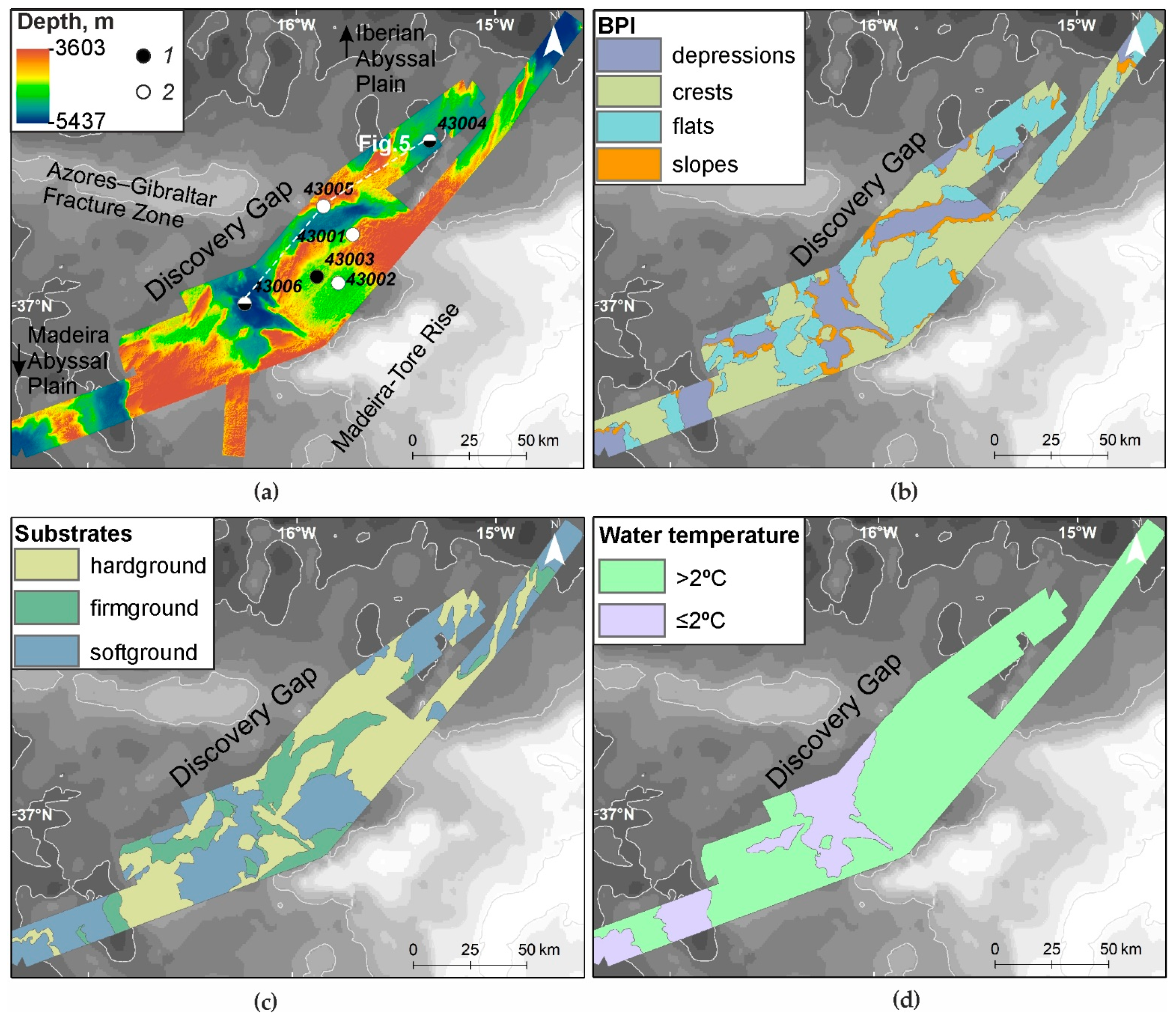
2.1.1. Bathymetric Position Index

One possible method of characterizing benthic landscapes, and their spatial variability, is through the use of the Bathymetric Position Index (BPI) [31]. BPI allows for automatic determination of mesoscale relief based on multibeam bathymetry.

The BPI is a derivative of the second order from the bathymetry and determines the elevation position of the point on the area in relation to the specified neighborhood. Negative values characterize depressions (the cell is lower than neighboring areas), positive values characterize elevations (the cell is higher than neighboring areas), near-zero values correspond to flat terrain and slopes.

For the BPI calculation, the GIS-application Benthic Terrain Modeler was used in the ArcGIS [32]. The BPI was applied to the digital elevation model (DEM) constructed on the basis of open access multibeam bathymetry data [33], Figure 2a. The BPI raster was created with the same resolution based on DEM.

The large-scale relief was determined with a large neighborhood radius to avoid the “noise” of the small-scale features, which means that the Broad Scale BPI (B-BPI) was calculated with a relatively large-scale coefficient. The optimal values for the outer and inner neighborhood radii were calculated based on the mean sizes of large- and small-scale relief forms measured in ArcGIS (

Table 1. Parameters, used for the calculation of the Broad Scale Bathymetric Position Index (B-BPI).

Parameter	Value
Digital Elevation Model resolution, m	100
Neighborhood form	ring
Outer radius, number of sells	200
Inner radius, number of sells	20
Scale coefficient	20,000
Minimum incline value for the slope, degree	3

).

Slopes and horizontal surfaces (flats) with BPI values closer to zero were differentiated using the slope raster. The latter was calculated in ArcGIS based on DEM. A threshold value (Table 1) was determined based on the graph of the slope value distribution.

The four mesoscale relief forms (BPI Zones) were determined based on standardized B-BPI values (B-BPIstd). The forms are referenced as landscape types:

• Crests—areas on the elevations with B-BPIstd ≥ 1;
• Depressions—areas in the lowering of the relief, B-BPIstd ≤ −1;
• Horizontal surfaces (Flats)—areas of the terrain with −1 < B-BPIstd < 1 and slope lower or equal to 3°;
• Slopes—areas of the inclined bathymetric surface with −1 < B-BPIstd < 1 and slope higher than the threshold value for slope.

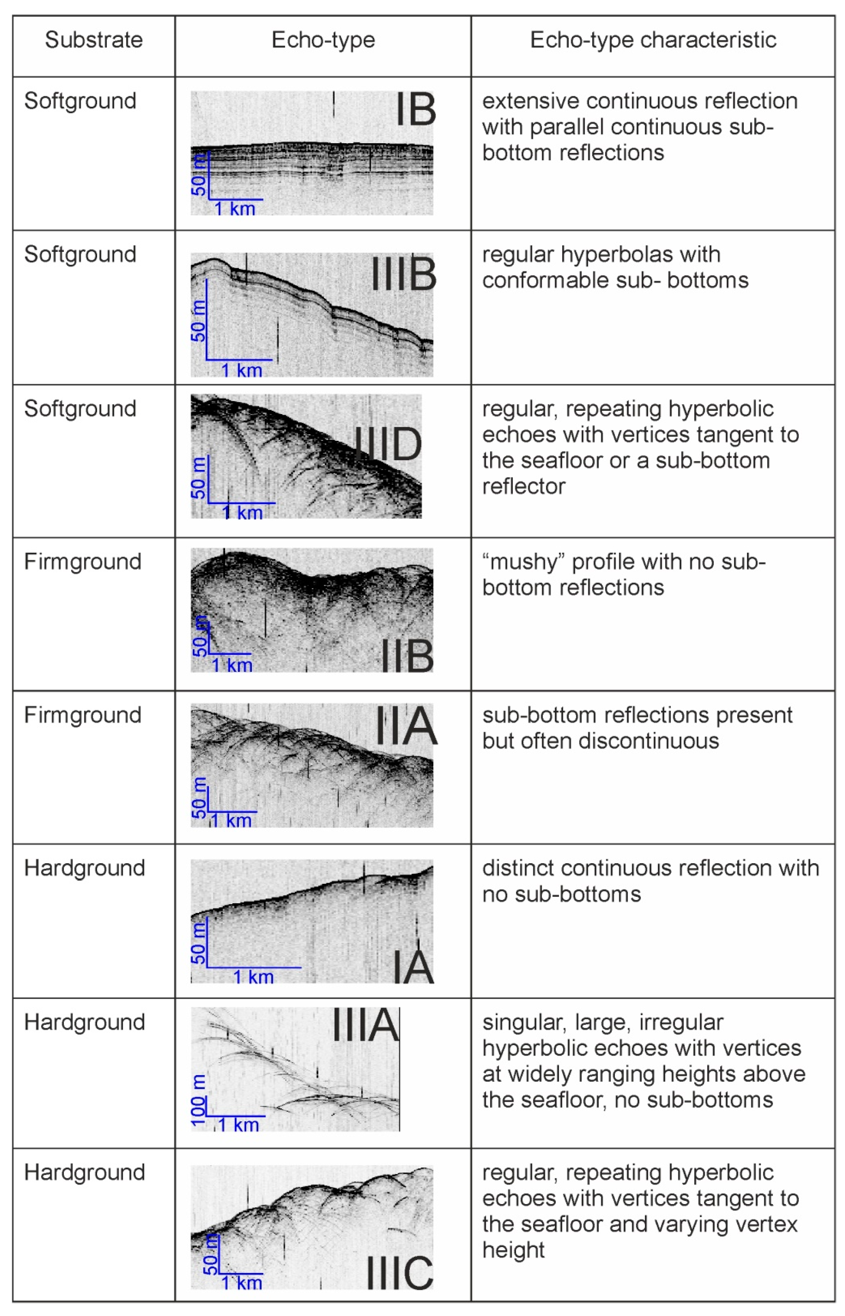
2.1.2. Bottom Substrates

Substrate type plays a major role in benthos and trace fossil distribution. The base substrates are softground, firmground, and hardground [34,35,36]. Due to the absence of the side-scan data in the area and limited sediment sampling sites (three gravity cores), the bottom substrates were extracted from the echotype distribution. The echotypes are taken from [14] where they were determined from sub-bottom profiles acquired with an EdgeTech 3300 Chirp profiler (2–8 kHz). An acoustic profile is characterized by weak penetration through sediments but with a high resolution that can capture details of the sedimentary record (e.g., [37]). Hardground is an acoustical basement of the high-frequency profiler and appears as distinct, sharp bottom echoes without sub-bottom reflectors. Firmground is characterized by echoes similar to those of the hardground but with increased signal penetration and more “mushy” profiles. Softground promotes even deeper signal penetration into the fine-grained sediments, seen as layers on the echograms, sometimes with overlapping of hyperbolas where the surface is wavy (sediment waves) [37]. Based on signal type, the eight echotypes originally defined in [14] were converted into three bottom substrate types: softground, firmground, and hardground (Figure 2c and Figure 3). The softground includes echotypes IB (extensive continuous reflection with parallel continuous sub-bottom reflections), IIIB (regular hyperbolas with conformable sub- bottoms) and IIID (regular, repeating hyperbolic echoes with vertices tangent to the seafloor, or a sub-bottom reflector). The firmground consists of echotype IIB (“mushy” profile with no sub-bottom reflections) and echotype IIA (sub-bottom reflections present but often discontinuous). The hard ground comprises three echotypes: IA (distinct continuous reflection with no sub-bottoms), IIIA (singular, large, irregular hyperbolic echoes with vertices at widely ranging heights above the seafloor, no sub-bottoms), and IIIC (regular, repeating hyperbolic echoes with vertices tangent to the seafloor and varying vertex height).

2.1.3. Water Temperature, Oxygen, and Suspended Particulate Matter Concentration

The hydrological measurements (near-bottom potential temperature, oxygen and suspended particulate matter concentration) were conducted at the five oceanographic stations (Figure 2a,

Table 2. Hydrological measurement and sediment core locations and type of data.

Station Number	Latitude	Longitude	Type of Data	Core Length, cm
ANS-43001	37°18.30′ N	15°42.51′ W	Hydrologycal
ANS-43002	37°06.73′ N	15°46.70′ W	Hydrologycal
ANS-43003	37°08.23′ N	15°53.07′ W	Sediment core	302
ANS-43004	37°40.75′ N	15°19.69′ W	Hydrologycal/sediment core	195
ANS-43005	37°24.97′ N	15°51.27′ W	Hydrologycal
ANS-43006	37°01.56′ N	16°14.45′ W	Hydrologycal/two sediment cores (A, B)	395 (A), 391 (B)

). Water temperature was acquired using the SBE 19plusV2 SeaCAT CTD-probe with measurements taken at 25–50 m above the sea bottom [38]. According to the classical definition from [39], AABW is water with a potential temperature lower than 2.0 °C. We used the 2.0 °C isotherm as the upper boundary of the AABW to define the spatial area of its influence in Discovery Gap.

Oxygen and suspended particulate matter (SPM) in the near-bottom waters were measured at the same oceanographic stations and the same depths as water temperature. The water was collected using Niskin bottles on the Carousel Water Sampler SBE 32. The dissolved oxygen in the water was measured onboard by the standard Winkler Method [40]. The SPM was estimated as its dry weight concentration from filtration onboard through a 0.45 µm pore size polycarbonate membrane filter [41]. The mean value of two filters was used for each sample, except for the ANS-43005 sample where the measurement came from only one filter. SPM residing on the filters includes both organic and mineral particles (e.g., [41,42]). Particulate organic carbon (its quantity and quality) was not studied separately.

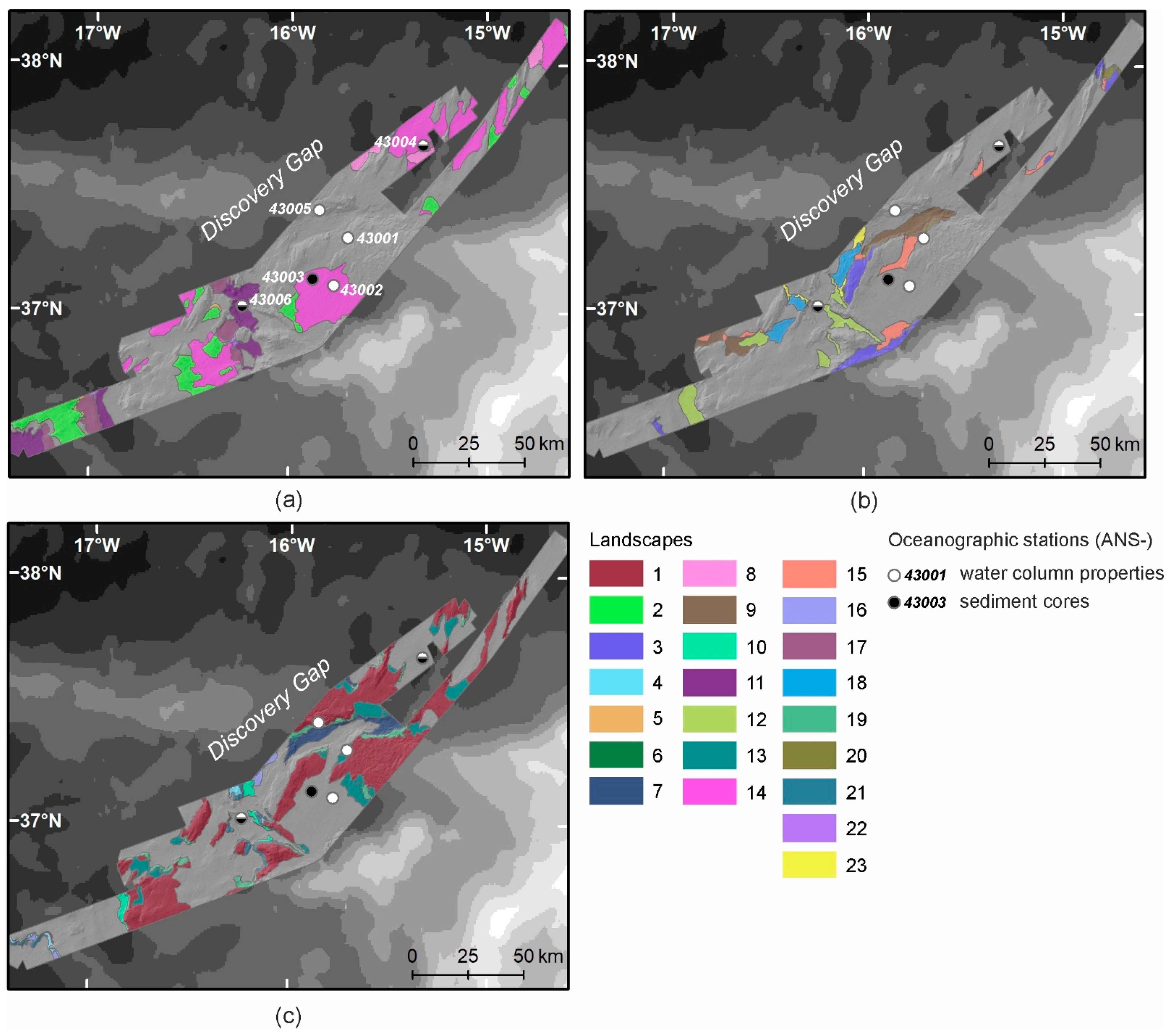
2.1.4. Landscape Mapping

A landscape map was created in the ArcGIS software by combining the shape-layers of the following components:

• Mesoscale relief defined with the BPI (crests, depressions, flats, slopes);
• Bottom substrate types (softground, firmground and hardground);
• Near-bottom water potential temperature with 2 °C as threshold value representing the upper boundary of the AABW.

Each landscape type has distinct boundaries and is defined by the combination of the abiotic components.

We did not use one of the main components of the landscape–benthic organisms, due to the absence of biological data in the area. This is because of the difficulties associated with their retrieval from great abyssal depths. Consequently, the landscape mapping was based only on the abiotic components, however, the results of ichnological studies in the sediment cores were used for indirect estimation of the biodiversity and benthic organism behavior.

2.2. Sediment Cores

We analyzed four sediment cores collected during the 43rd cruise of the R/V “Akademik Nikolaj Strakhov” in 2019 ([38], Figure 2a, Table 2). Two cores (ANS-43006_A and ANS-43006_B) were retrieved from the ANS-43006 site for their simultaneous analysis in different laboratories. The thorough study of the cores included stratigraphic subdivision, facies analysis and an interpretation of the sedimentary processes is presented in [14]. According to the study, sediments in all the cores encompass the last 240 ka and correspond to seven marine isotope stages (MIS 7-1). Identified sedimentary facies reflect significant variability of the upper boundary and current velocity of the AABW which were proposed to relate to the glacial-interglacial climatic changes during the Quaternary. Intensified AABW currents accompanied by increased carbonate dissolution and high terrigenous supply to the core sites were registered during glacial intervals (MIS 6, 4, and 2) and at their terminations. Revealed processes reflect long-term environmental dynamics which may significantly influence the composition of sediment cores.

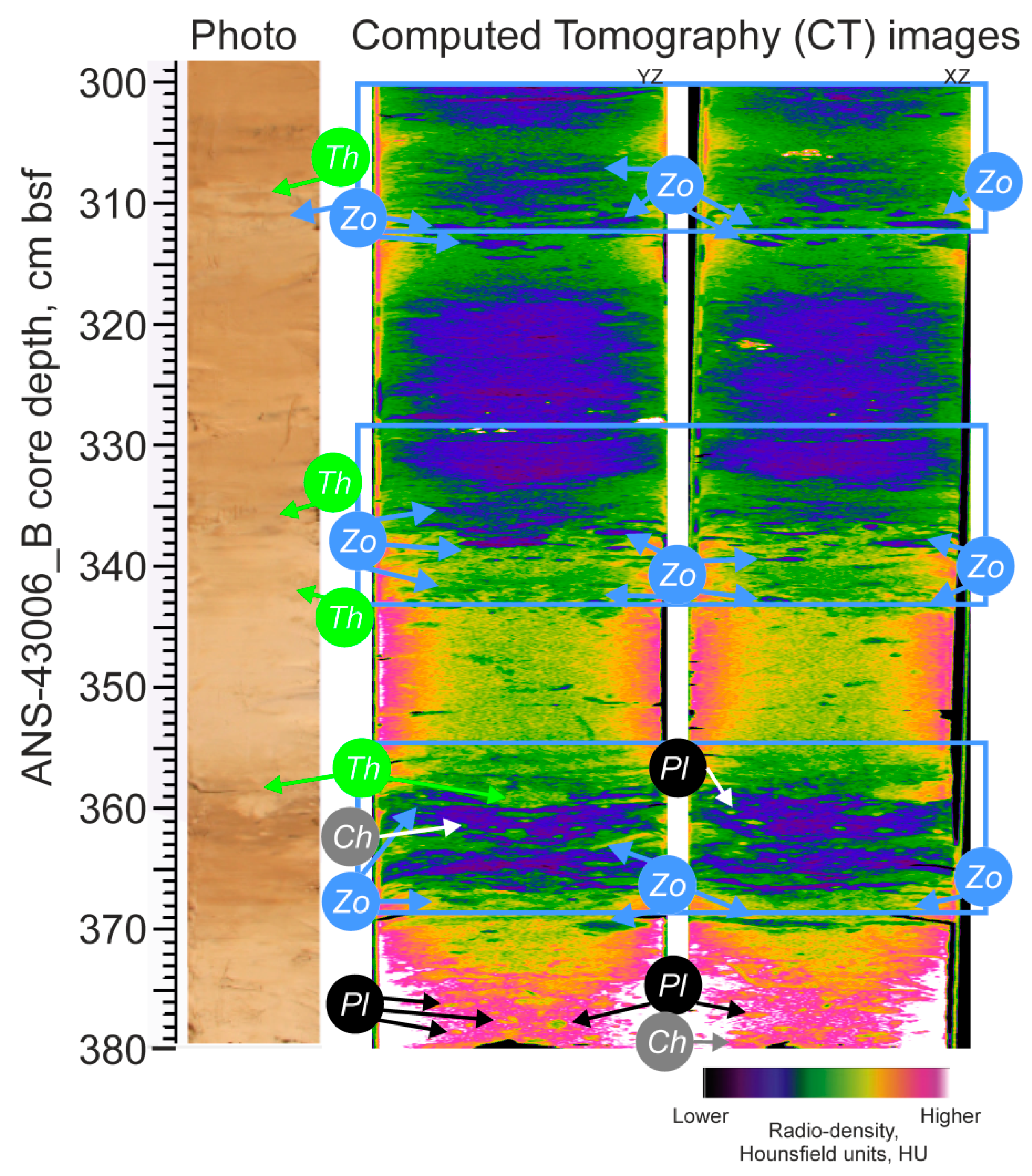
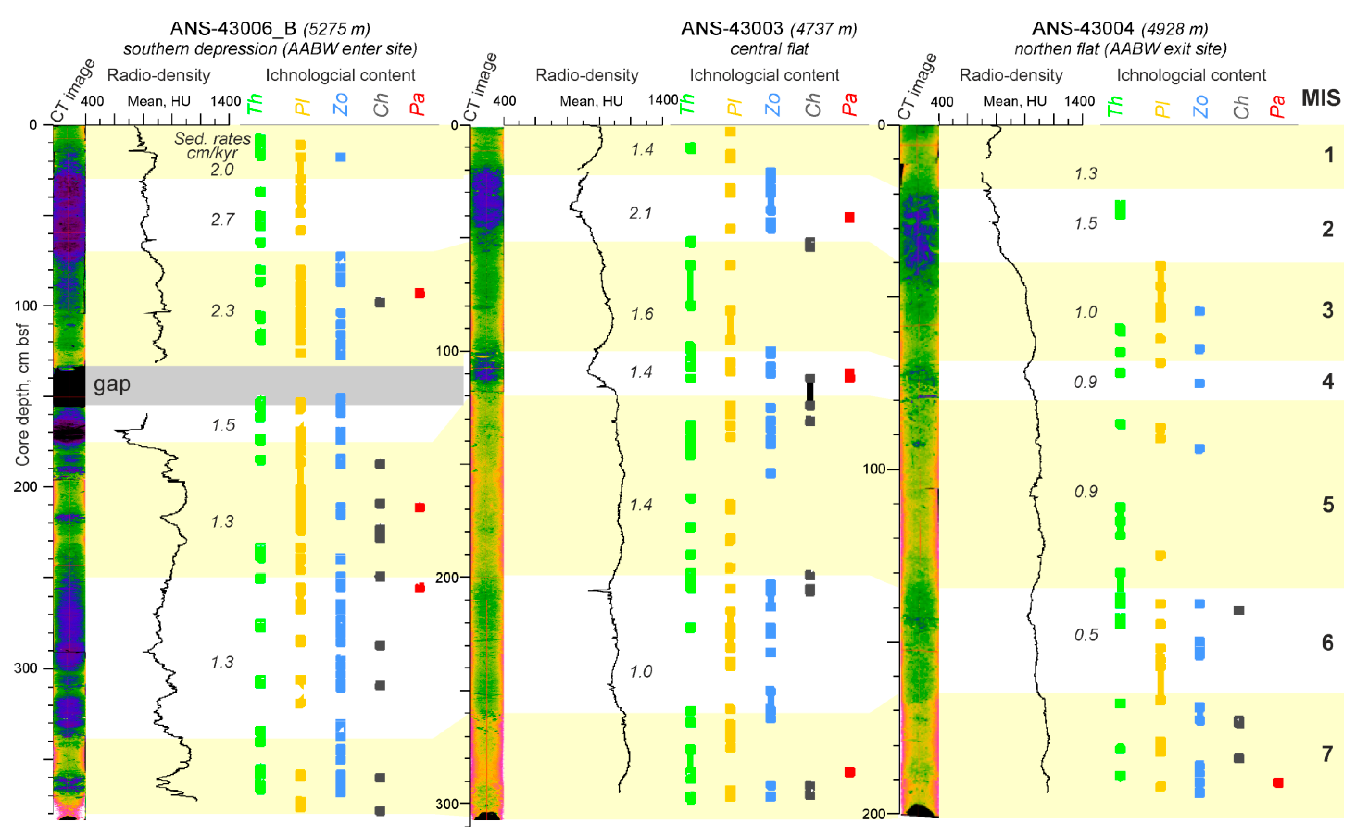
2.2.1. CT-Scanning

Before opening, the ANS-43003, ANS-43004, and ANS-43006 B cores were analysed using clinical Computerized Tomography equipment (HITACHI ECLOS 16 Multislice CT) at the Veterinary Teaching Hospital Rof Codina in Lugo (Galicia). The data were collected following the acquisition protocol of [43]. The final resolution per voxel is 0.2 mm × 0.2 mm × 0.65 mm (x, y, z). Radio–density profiles for the cores were calculated using the software anidoC [43]. Tomographic pictures from the cores were obtained using MRicro [44]. These pictures present the same radio-density colour scale and hence, colours from the different cores are directly comparable. A 25 cm gap at 130–155 cm core depth (cm below seafloor, cm bsl) was discovered in the ANS-43006_B core upon opening, which is seen as a black space on the computed tomography image.

2.2.2. Ichnology

The ichnological analysis was conducted on high-resolution digital images and computer tomography (CT) data. To enhance the visibility of trace fossils in modern cores, like those studied here, digital images were processed using the high-resolution image treatment recently proposed ([45,46,47,48]). Images were treated, controlling image levels of brightness, contrast, vibrance, and saturation ([45] for details). CT scan images increase the visibility of trace fossils in particular cases, especially when the infilling material of trace fossils is different to the host sediment.

As usual for ichnotaxonomical analysis in cores, trace fossils were characterized at the ichnogenus level by the recognition of diagnostic features [49]. Special attention was paid to the general shape, size, orientation, internal structures and their infilling material. Moreover, other ichnological attributes such as the distribution of traces, ichnodiversity, cross-cutting relationships, tiering structure, relative abundance, and degree of bioturbation, as a percentage of bioturbation within a vertical section or bioturbation index for any ichnogenera or the complete trace fossil assemblage, were considered [48,50,51].

2.2.3. Benthic Foraminifera

BF (calcareous and agglutinated) were studied from the top 30 cm of the sediment cores ANS-43004 and ANS-43006_A to establish possible differences in abyssal faunal composition and biodiversity. The two cores were chosen as they are located in the AABW entrance and exit sites of the gap. We did not analyse the core ANS-43003 to exclude the expected error caused by the enhanced preservation of calcareous microfossils due to the weaker dissolution effect at shallower depths.

The top 30 cm of the cores were sampled at 10 cm (1-cm thick slices). This corresponds to Marine Isotope Stage 1 (MIS 1) and a time period of about 0–12.9 ka for core ANS-43004 and 0–10.5 ka for core ANS-43006_A according to the age model, presented in [14]. Samples were washed through a 63 μm sieve and subsequently, the dry coarse fractions were passed through a 100 μm sieve. Over 300 specimens of benthic foraminifera from the >100 μm fraction were counted and identified to species level under the Olympus SZX16 microscope following the standard approach (e.g., [52,53,54]).

Several independent proxies have been used to evaluate benthic foraminiferal variability:

5.

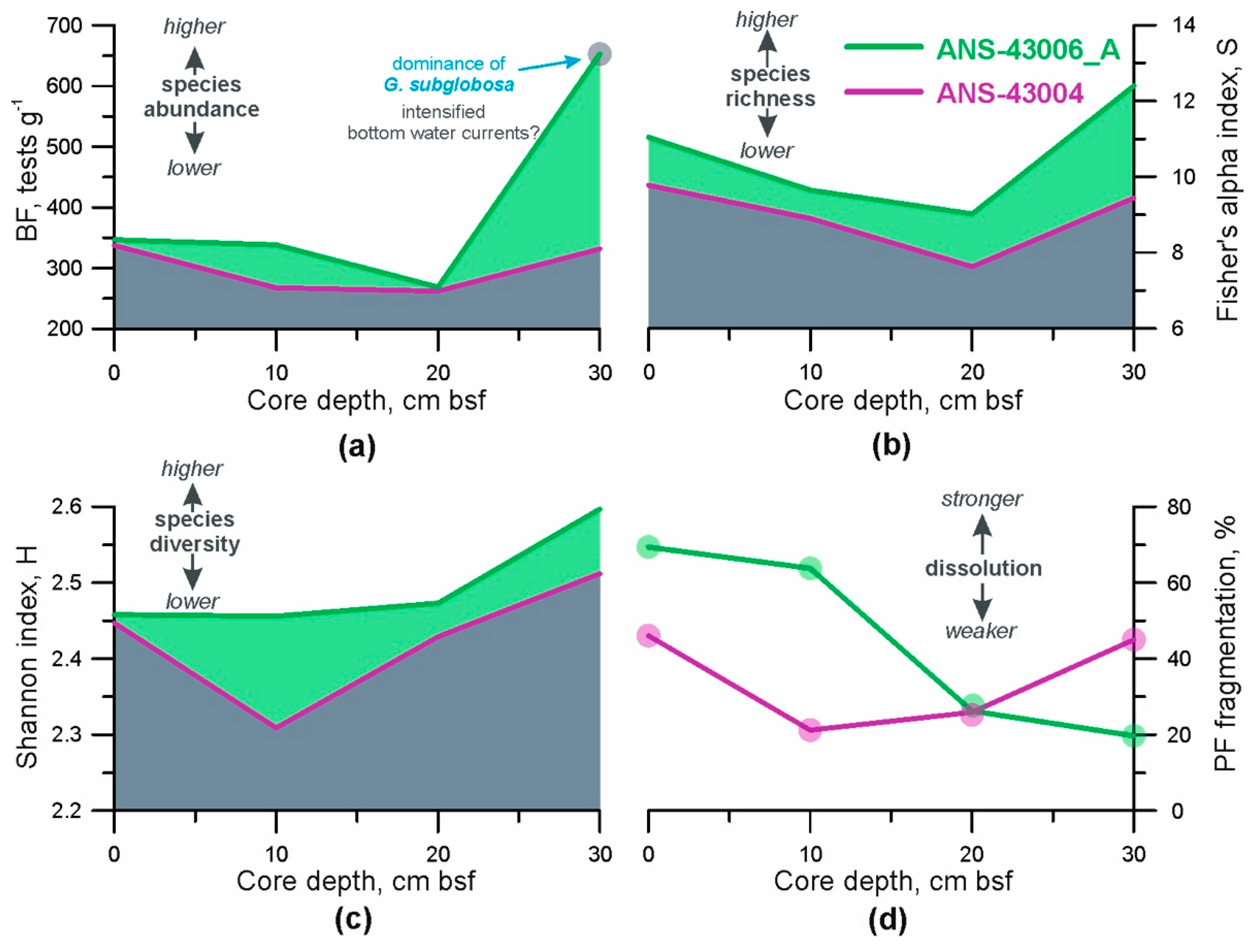
Total BF abundance. This parameter was calculated as the number of benthic foraminifera per 1 g of dry bulk sediment [55]. A combination of sufficient food supply to the seafloor and relatively high oxygen content in the pore and bottom water creates favourable conditions for mass development of benthic organisms (e.g., [18,21]). Consequently, under such conditions, the concentration of BF tests in the sediments should be higher;

6.

BF ecological indices. The Palaeontological Statistics (PAST) data analysis package was applied to the foraminiferal data (the number of each BF species at given depths in the cores) to obtain the distribution patterns of two ecological indices [56]. The Shannon index (H) accounts for both the number of taxa and the individuals in a community, so here we use it as a parameter of heterogeneity (diversity) of each sample [57]. Fisher’s alpha diversity index (S) describes the relationship between the taxa and the number of individuals of those taxa [58] and consequently, reflects the species richness ([57,59]);

7.

Fragmentation index of planktic foraminifera (PF). It is well-known that changes in foraminiferal abundances are commonly affected by dissolution in the deep open ocean (e.g., [27,60]). Therefore, it is necessary to consider how strong the past dissolution signal might have been and whether it predominated over the export productivity and lateral food advection. The PF fragmentation index was used as a dissolution proxy and calculated according to the equations formulated by [61]. We counted planktic foraminifera in the >150 μm sediment fraction which is considered to be the most sensitive to changes in hydrological conditions (e.g., [62]). A PF fragment was defined as a test portion less than 60% of its original size [62]. If a relationship between the curves of total BF abundance and PF fragmentation index can be identified then it may be possible to suggest that dissolution plays a major role in BF distribution. A higher value of PF fragmentation, together with increased content of pitted benthic foraminifera shells in the same sample, indicates stronger dissolution.

2.3. Integration of the Data

The landscape maps, including studies on oceanographical parameters, were produced to evaluate the abiotic parameters and their changes through the gap (e.g., [63]). Furthermore, the ichnological and benthic foraminifera data were compared with the abiotic variables to eliminate their influence on them.

3. Results

A total of 9404.5 km² were mapped and 23 seabed landscapes were identified in Discovery Gap (Figure 4,

Table 3. Seabed landscapes resulted from the overlay of the BPI, substrate types, and water temperature. The percentage distribution of the landscapes in the area is marked by greyscale from high (dark grey) to low (white) values. Italian style highlights the landscapes with water temperature ≤2 °C.

Number	Landscape	Area, km2	Area, %
1	Crests, hardground, water temperature >2 °C	2704.7	28.8
2	Crests, softground, water temperature >2 °C	767.3	8.2
3	Crests, firmground, water temperature >2 °C	334.4	3.6
4	Crests, hardground, water temperature ≤2 °C	58.9	0.6
5	Crests, softground, water temperature ≤2 °C	20.8	0.2
6	Crests, firmground, water temperature ≤2 °C	7.4	0.1
7	Depressions, hardground, water temperature >2 °C	235.4	2.5
8	Depressions, softground, water temperature >2 °C	161.9	1.7
9	Depressions, firmground, water temperature >2 °C	333.2	3.5
10	Depressions, hardground, water temperature ≤2 °C	110.8	1.2
11	Depressions, softground, water temperature ≤2 °C	512.6	5.5
12	Depressions, firmground, water temperature ≤2 °C	350.5	3.7
13	Flats, hardground, water temperature >2 °C	518.0	5.5
14	Flats, softground, water temperature >2 °C	1902.8	20.2
15	Flats, firmground, water temperature >2 °C	273.4	2.9
16	Flats, hardground, water temperature ≤2 °C	52.0	0.6
17	Flats, softground, water temperature ≤2 °C	299.9	3.2
18	Flats, firmground, water temperature ≤2 °C	205.1	2.2
19	Slopes, hardground, water temperature >2 °C	282.4	3.0
20	Slopes, firmground, water temperature >2 °C	71.7	0.8
21	Slopes, hardground, water temperature ≤2 °C	117.3	1.2
22	Slopes, softground, water temperature ≤2 °C	21.7	0.2
23	Slopes, firmground, water temperature ≤2 °C	62.3	0.6

). The significant variety in bottom landscapes occurs as a result of the complex relief, sediment distribution (patchiness) and AABW distribution in the gap.

3.1. Relief and Substrate Types

Crests are the most extensive relief type in the area and comprise 41% of all relief. They are mostly represented by hardground (71%); firmground and softground comprise 9% and 20%, respectively (Figure 4). Crests with hardground have large areas of sediment absence and bedrock exposure on the sea bottom. These areas are associated with the ridges of the Gloria Fault and Madeira Tore Rise and with isolated, typically SW-NE trending, elongated ridges within the gap.

The next most widespread relief type is flats. They account for 34% of the area and are represented by softground (68%), hardground (18%) and firmground (15%) (Figure 4). Flats correspond to terraces along the Gloria Fault and Madeira Tore Rise. They are also typical of the Madeira and Iberian Abyssal Plains within the study area.

Depressions and slopes account for 18% and 6% of the bottom relief in the study area, respectively. Depressions in the gap are mainly represented by soft and firmground (40% of each substrate type), while hardground constitutes 20%. There are three large depressions in the southern, central and northern parts of the gap that are separated by sills (central and northern sills). The southern depression is represented by softground. It has an irregular form and is separated from the Madeira Abyssal Plain by an elevated relief of crests and flats. The central depression is a narrow SW-NE elongated feature and is characterized by the firmground. The northern depression is located on the Iberian Abyssal Plain and is represented by a flat bottom according to the BPI classification and characterized by softground.

Slopes are almost exclusively characterized by hardground (89%), firm- and softground account for the 6% and 5% of the bottom substrates, respectively. Slopes within the gap are typically very narrow and steep and usually bound the depressions.

3.2. Temperature, Oxygen and SPM Concentration in the Near-Bottom Waters

During the 43rd cruise of the R/V ANS (2019), the coldest potential water temperature (1.993 °C) was measured in the entering (southern) depression, while at the exit of the gap (northern depression) the measured near bottom potential water temperature was higher. At a depth of 4735 m, it was 2.00 °C in the southern depression (station ANS-43006) and 2.01 °C at the same depth in the northern depression (station ANS-43004, Figure 5). Unfortunately, the water temperature was not measured in the central depression in 2019, but from literature and public data, we know that it is higher than 2.0 °C [64,65,66].

SPM concentrations in the near-bottom waters show a similar pattern (

Table 4. Suspended particulate matter (SPM) concentration and oxygen in the near-bottom waters in Discovery Gap.

Station	Depth, m	SPM, mg/L	Oxygen, mL/L
ANS-43001	4533	0.034	5.30
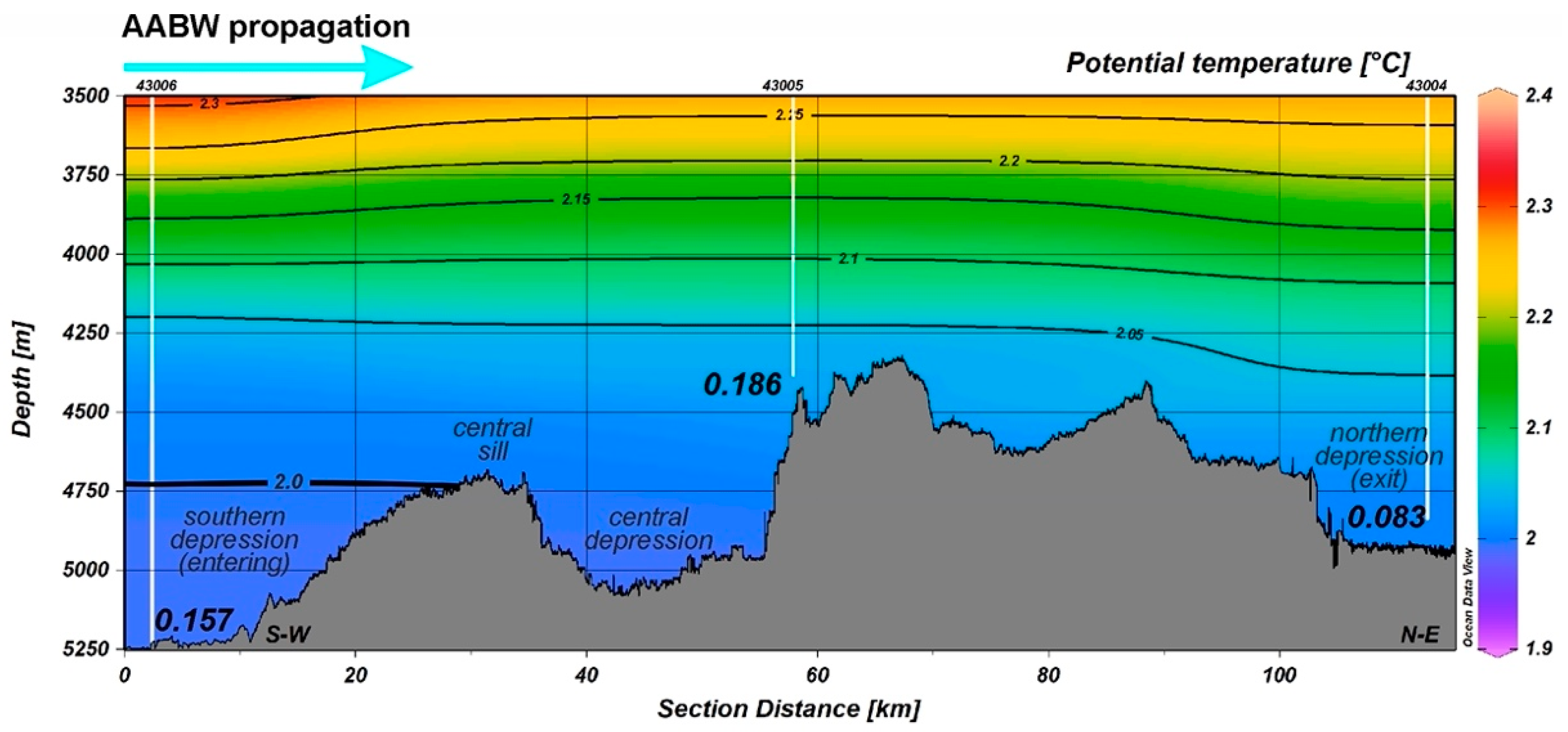
ANS-43002	4673	0.145	5.69
ANS-43004	4840	0.083	5.32
ANS-43005	4384	0.186	5.61
ANS-43006	5250	0.157	5.29

, Figure 5). Increased values were measured in the southern part of the gap: 0.175 mg/L in the southern depression and 0.145 mg/L at the flat (terrace) of the Madeira-Tore Rise. The highest value was registered at the crest of Gloria Fault ridge to the west of the northern deep—0.186 mg/L. This is the shallowest station with a depth of about 4400 m (Table 4). The lowest value was identified at the crest to the east of the central depression (0.034 mg/L). At the northern exit of the gap (northern depression), the near-bottom SPM concentration was as low as 0.083 mg/L.

Oxygen concentration in the near-bottom water is quite uniform and varied from 5.29 to 5.69 mL/L with the mean value of 5.44 mL/L (Table 4). There is no visible trend in the oxygen distribution throughout the gap. The bottom-water oxygen level appears to be relatively homogeneous and dissolved oxygen in the near-bottom waters is near saturation levels that correspond to oxic conditions.

3.3. Ichnology

In all the cores, trace fossil assemblages are quite homogeneous, mainly consisting of Thalassinoides, Planolites and Zoophycos, together with frequent Chondrites and rare Palaeophycus (Figure 6). This assemblage can be assigned to the Zoophycos ichnofacies. The Zoophycos ichnofacies is mainly characterized by feeding structures, as are found in the present case study; Chondrites is related to different feeding behaviors (i.e., deposit-suspension-detritus-feeding and even chemosimbiosis), Palaeophycus is interpreted as a dwelling or suspension-feeding structure, Planolites is considered to be produced by deposit-feeders, Thalassinoides is excavated as dwellings, associated with combined suspension- and deposit-feeding behavior and Zoophycos is mainly related to deposit-feeding behavior [49].

Trace fossils are relatively abundant in all the studied cores (ANS-43003, ANS-43004 and ANS-43006 B), showing well-defined framework burrow systems (i.e., Thalassinoides) and cross-cutting relationships. This fact can be associated with a well-developed trace maker community that can be interpreted as revealing generally good environmental conditions in terms of oxygenation, nutrient availability and continuous sedimentation. In this context, however, stratigraphic variations in the percentage of trace fossils are observed in the three analyzed cores, from intervals characterized by scarce, near absence, discrete trace fossils, with 0–5% of the bioturbated surface, to intervals showing an amount of trace fossils, in which more than 60% of the vertical section is bioturbated.

In this general context, some variations in the relative abundance of ichnogenera, including presence/absence, can be observed between and within the studied cores. Thus, in sediment cores ANS-43003 and ANS-43004 Thalassinoides, and Planolites are usually the most abundant traces, while in ANS-43006 the most abundant through the core is Zoophycos (Figure 7).

The ichnological studies also demonstrate the lateral difference in the macrobenthic tracemaker community due to environmental changes in the gap (Figure 7). Located at the entrance of the gap, the ANS-43006 core is characterized by the highest tracemaker presence, especially Planolites and Zoophycos, in comparison with the other two cores. Chondrites are also abundant. In the ANS-43003 and ANS-43004 cores, the number of traces decreases with a minimum in ANS-43004.

3.4. CT-Scanning

CT images are useful for the visual characterization of the cores and in aiding the identification of ichnological taxa in alongside photo images [43]. Quantitative analysis of CT-scan data allows numerical comparison of the cores according to the radio-density values in the HU scale.

The mean radio-density values of each slice through the ANS-43006, ANS-43003 and ANS-43004 cores range between 605 and 1206 HU, 820 and 1194 HU and 658 and 1167 HU, respectively (Figure 7). The radio-density varies significantly between glacial and interglacial times according to the stratigraphic subdivision presented in [14]. The difference reflects changes between high calcareous interglacial intervals (odd Marine Isotopic Stages, MIS) characterized by high radio-density values and low calcareous glacial intervals (even MIS numbers) with low HU values.

In the ANS-43006 sediment core, the mean radio-density values vary considerably between the interglacial periods (MIS 7, 5, 3, 1) and glacial (MIS 6, 4, 2) and comprise 953 HU and 830 HU, respectively (Figure 7). The ANS-43003 and ANS-43004 sediment cores are characterized by smoother tomographical trends (Figure 7). The average radio-density value for the interglacials is 1076 HU and 996 HU for the glacial in the ANS-43003. In the ANS-43004 core, the tomographical difference between glacial and interglacial intervals is even less. The mean CT-scan radio-density value for the interglacials is 1002 HU and for the glacials it is 967 HU.

3.5. Benthic Foraminifera

Micropaleontological analysis of the sediment samples in the >100 µm fraction enabled the identification of more than 60 BF species in core ANS-43006_A and more than 50 BF species in core ANS-43004. Within the top part of the cores, corresponding to MIS 1, the BF assemblages consist mainly of the six species typical of abyssal environments ([18,67]). These species (Alabaminella weddellensis, Eggerella bradyi, Epistominella exigua, Globocassidulina subglobosa, Nuttallides umbonifera, and Oridorsalis umbonatus) together account for about 70% of the faunal relative abundance in most samples (Supplementary Materials Table S1).

Total BF abundance and diversity information is presented in Figure 8. In all the samples, the values of diversity indices (Fisher’s alpha index (S) and Shannon index (H)) are found to be higher in core ANS-43006_A in relation to the ANS-43004 data (Table 2). The H values vary within a limited range of 2.31–2.60 in the studied parts of the cores. The S values are positively correlated with total BF abundances and are greatest at 29–30 cm bsf in both cores. The BF abundance is usually about 260–350 tests per 1 g of dry sediment, however, one distinct maximum (650 tests g⁻¹) is detected within the core ANS-43006_A at about 10.5 ka (29–30 cm bsf). The PF fragmentation index is highly variable at 20–69% and 21–46% in cores ANS-43006_A and ANS-43004, respectively. An inverse correlation between the BF abundance and PF fragmentation percentage is observed in core ANS-43006_A (Figure 8a,d). No such relationship is observed between these two curves in ANS-43004, i.e. fragmentation maxima at 0 and 30 cm do not coincide with the BF abundance minima (Figure 8a,d).

3.6. Seabed Landscapes

A combination of the relief peculiarities, sediment patterns, and near-bottom water potential temperature distribution allows us to define the landscapes in Discovery Gap. Crests represented by hardground with near-bottom water temperature >2 °C cover the largest area in the gap (2704.7 km², 28.8%). The second most extensive landscape is flats covered by softground with near-bottom water temperature >2 °C. They occupy an area of 1902.8 km², which is 20.2% of the study area.

The landscapes covering less than 1% of the area of the gateway are mainly slopes and crests with different substrates and near-bottom water temperatures <2 °C. Areas of depressions and flats with near-bottom water temperature <2 °C vary between 0.6 and 5.5% depending on substrate type. The depressions with near-bottom water temperature <2 °C are located southward of the central sill and cover 10.4% (973.9 km²) of the study area. Flats of different substrate types but with near-bottom water temperatures lower than 2 °C are also located to the south of the central sill and amount to 6% (557 km²) of the gap’s area.

Sampling sites of the sediment cores are located along the direction of the AABW propagation through the gap and the cores relate to the two different landscapes (Figure 1 and Figure 4). The ANS-43006 site is located in the region where AABW enters the gap and corresponds to the depression with the softground substrate and near-bottom water temperature less than 2 °C. The ANS-43003 sediment core was retrieved from the central part of the gap on the terrace (flat) of the Madeira-Tore Rise. The site is characterized by soft sediments but the near-bottom water temperature is higher than 2 °C. ANS-43004 was retrieved from the flat area outside of the northern exit of the gap which is characterized by softground and a near-bottom water temperature greater than 2 °C.

4. Discussion

4.1. Landscapes Variability in the Deep-Water Gateway

A high diversity of landscapes in Discovery Gap is detected. This increased patchiness compared to surrounding abyssal plains may lead to enhanced habitat heterogeneity which in turn may promote high biodiversity in the gap. The five most important factors of benthic biodiversity in the deep sea were identified at the regional (landscape) scale by Levin et al. [68]: food input, bottom water flow, bottom-water oxygen levels, sediment heterogeneity and ecological disturbance. Below, we examine the biodiversity potential in the Discovery Gap gateway from these perspectives.

In the deep-sea environment, the food supply is mainly brought down from the euphotic zone by a biologically driven downward flux of organic matter (e.g., [69]). Discovery Gap is quite a small region relative to the surface circulation system of the Azores Current, which could influence the primary production of organic matter. The gap area lies within a single biogeochemical province [70]. Therefore, we assume that there is no significant difference in organic matter supply to the gap area from the surface sources. However, a lateral variability of nutrient distribution within the gap could exist because of the influence of the bottom currents that are discussed in Section 4.2.

Episodic disturbances, that in the abyssal zone are mainly due to turbidity flows, are also not recognized in the study area as sedimentation is continuous from the Late Pleistocene to Holocene in the sampled sediment cores [14]. However, the Azores–Gibraltar Fracture Zone, and especially the East Gloria Fault region, is known to have a record of high to very high magnitude earthquakes, with the latest recorded in the 20th century [71], which may be responsible for the earthquake-triggered slides and associated debris flows and turbidity currents [72]. No sediment disturbance was found, at least not in the sediment cores. Moreover, Zoophycos ichnofacies prevailing in the studied cores is typical for the distal, deep environments which are usually quiet environments with an absence of turbiditic currents [73,74]. However, we cannot exclude that there may be alternative turbidity current routing pathways from surrounding topographic highs [14] possibly represented by softground. From the ichnological point of view, the different ichnotaxa may occupy both continuously deposited contourites, pelagic sediments, and event dependent turbidites (e.g., [75,76]).

The most heterogeneous abiotic factor that may result in increasing biodiversity in Discovery Gap is a topography that is associated with sediment patchiness and substrate variety. The geology and sedimentary processes in Discovery Gap are described in detail in [14]. In the present study, the indirect measurement of the infaunal organisms based on the ichnological and benthic foraminifera studies in the upper parts of the two cores are presented. The intense bioturbation in the three sediment cores reflects the presence of deposit feeders and possibly surface feeders [16] in the soft sediments of the depressions and flats of the gap. Moreover, the difference in the ichnological content between the cores reflects different living strategies of the endofauna along the gap, which is discussed in Section 4.2. Large areas of flats and depressions in the gap presented by soft- and firmground substrates with oxic near bottom conditions are potentially favorable for endobenthic organisms ([16,34]). The sparseness of these areas through the gap and their separation by sills and elevations may break up the benthos communities and lead to elevated species diversity through the gap (e.g., [11,77,78]).

The 43% of the area with hard bottom exposures mostly corresponds with the crests and slopes of Discovery Gap presenting hard substrate habitats for benthic organisms. As has been shown in previous studies, sessile fauna may be found on rocky outcrops of the continental margins and the Mid-Atlantic Ridge in the lower bathyal depths (800–3500 m depth) [78,79]. Little is known about the benthos of abyssal (4000–6000 m depth) hardgrounds that constitutes almost half of Discovery Gap area. Besides the rocky outcrops on the gap’s flanks, around 13% of the hardground exposures are observed within the gap. They are present not only on crests and slopes, which is unsurprising but also on the flats and depressions. We connect the absence of the soft sediment in the depressions and flats with the enhancement of the bottom current flow in the narrow parts of the gap and over the sills [8,9]. The intensification of bottom current velocities over the sills of Discovery Gap is confirmed by numerical modelling [80]. The acceleration of the bottom flow in these areas leads to sediment erosion, or rather nondeposition, and the formation of the firmground and hardground (Figure 4, Table 3). These abyssal rock patches may increase species diversity as, for example, is the case in the Vema Fracture Zone of the Mid-Atlantic Ridge [11], although, future work is needed to determine the hardground benthos in Discovery Gap. Studies of the abyssal biota are expensive and accompanied by technical difficulties (e.g., [3]). The landscape map presented in our study will be helpful in such research because the abiotic parameters and potential locations of the benthic fauna are described in detail.

4.2. Environmental Drivers of Ichnofossils and Benthic Foraminifera Spatial Variation in the Deep-Water Gateway

In deep-sea environments, the two main factors that influence tracemakers are presence of oxygen for respiration and presence of organic matter required for food [16]. According to our results, oxygen is distributed quite uniformly in the near-bottom waters throughout the gap, determining a general oxygenated setting with minor incidence on the benthic community. Due to the relatively small extent of the gap, the food supply by vertical flux from the epipelagic zone is assumed to be constant in space but may exhibit seasonal variability. The dominance of deposit-detritus-feeding behaviors support the hypothesis that the accumulation of organic particles in the sediment occurred mainly in tranquil waters. Therefore, the spatial variations of the near-bottom water propagation in the gap may be the main reason for the observed changes in ichnological diversity between the studied cores.

A particular characteristic of Discovery Gap (and any other deep ocean gateway) is that it causes the restriction of the bottom water propagation from one abyssal plain to another. Since bottom water with a potential water temperature less than 2.0 °C was found only in the southern depression, we assume that the central sill presents some kind of barrier within the gap which prevents the distribution of the coldest and heaviest AABW northward (Figure 2d and Figure 5). This restriction leads to a registered difference in water temperature between the southern and northern parts of the gap because (1) the coldest (<2.0 °C) and heaviest AABW cannot cross over the central sill and is arrested in the southern depression and (2) AABW mixes with the upper warmer waters during its movement through the gap [14].

The specific pattern of AABW propagation may cause variations in nutrient supply. Regions with increased bottom current (typically, contour current) intensity in the deep sea are characterized by elevated SPM that can carry a considerable amount of adsorbed organic carbon (e.g., [42,81,82]) which in turn feeds benthic organisms [83]. Overall reinvigoration of the sluggish abyssal AABW caused by the constricted topography of Discovery Gap was documented [14]. The values of SPM concentrations in the near-bottom layer in Discovery Gap are quite high and are even comparable to those measured in the surface waters (e.g., [84]). Additionally, the passing of AABW over the Canary Basin and Madeira Abyssal Plain during its northward propagation [9] may play a role in nutrient supply to Discovery Gap. These regions are known to be under the influence of the upwelling currents off NW Africa that can export offshore a significant amount of organic matter [85]. The increased SPM concentrations in the near-bottom water in the southern part of Discovery Gap (AABW entrance, station ANS-43006) and decreased in the northern exit (station ANS-43004) confirms the changes of the near-bottom current flow as it propagates through the gap (Figure 5). The highest value of SPM concentration observed on the ridge of the eastern segment of the Gloria Fault (ANS-43005, Table 4) may be explained by the resuspension of surficial sediments resulting from the presence of the water mass boundary at a depth of 4500 m between AABW and overlaying North Atlantic Deep Water [14] or/and the interaction of the flow with the ridge (e.g., [86]).

The blocking effect of the central sill is accompanied by a reduced capacity of the bottom current flow to carry the SPM from the southern entrance to the northern exit of the gap. Therefore, the northern flats probably received fewer nutrients than the southern depression which may explain the difference in the trace fossil assemblages and their abundance in the gap. Moreover, sediments near the gap entrance (ANS-43006) show higher sedimentation rates and more variable radio-density values (Figure 7) supporting increased suspended matter influx and enhanced bioturbation rates compared to the exit of the gap. Our results suggest that the shift in the near-bottom water parameters due to restricted AABW propagation influences the ichnological content of the sediments in the deep-water gateway. However, detailed studies of particulate organic matter composition and quality, and macrobenthic communities in the gap are needed to support this interpretation.

Despite the use of CT-scan data to aid ichnological description, the ichnological data cannot be readily compared with numerical CT-scan data directly. That is because the latter is strongly dependent on the other factors, such as grain size, sedimentary structures, distribution of particles, etc. (e.g., [43,87]). Variations in the tomographical data correspond to the glacial–interglacial changes in foraminifera content: increased during warm intervals and reduced during cold intervals. This variability is associated with the Late Pleistocene–Holocene climatic changes in surface productivity and the enhanced corrosive effect of the AABW during glacials (e.g., [14,88]). According to our results, the CT-scan values show the highest variability in core ANS-43006_B, where the lowest values are associated with increased foraminifera dissolution during glacials (Figure 7). Moreover, the sediments at the exit of the gap (ANS-43004) are characterized by overall higher radio-density values than at the entrance depression (ANS-43006) despite the comparable core sampling depths. This confirms the increased influence of the AABW in the entrance depression, not only in recent times but also through the Late Pleistocene–Holocene interval.

A comparison of prevailing benthic foraminiferal taxa in the upper sediments of the two deepest cores in the gap shows a common composition of BF species, but differences in their concentrations. The faunas were dominated (>70%) by A. weddellensis, E. bradyi, E. exigua, G. subglobosa, N. umbonifera, and O. umbonatus. Most of these species appear to be typical of oligotrophic environments, where a microhabitat close to the sediment-water interface and perhaps a suspension-feeding life strategy may be advantageous ([27,53,67]). Most of the BF species observed in this study are considered epifaunal and shallow infaunal, which are usually dominant in environments with well-oxygenated bottom waters ([21,89]). The similarities in BF species’ composition at the two sites suggests that the bottom-water and pore-water oxygen levels were not significantly changed between the core locations. Consequently, the BF assemblages are controlled mostly by a limited food supply and are subject to a dissolution effect due to the changes in bottom-water carbonate saturation (Figure 8). Taking into consideration the elevated values of total BF abundance in relation to lowered values of PF fragmentation in core ANS-43006_A, we propose that this deeper sediment core experienced heightened dissolution. However, the statistical analysis in the PAST software has identified higher foraminiferal diversity and species richness within the upper sediments of the deeper southern core ANS-43006_A despite the stronger dissolution effect on the carbonate shells according to PF data. In the shallower northern core ANS-43004, the ecological parameters of BF assemblages were markedly lower though the dissolution decreased. We assume that this difference is likely to result from the unequal BF productivity conditions over the two core sites. Given that vertical organic matter fluxes exported from the photic zone to the bottom are supposed to be comparable for the relatively small area of Discovery Gap, we suggest that lateral transport of nutrients played a major role in shaping the difference in the BF community structure between the cores. The somewhat similar values of total BF abundances in the cores might be explained by the influence of the more corrosive water mass that is present below the depth 5000 m over ANS-43006_A site. A peak in carbonate dissolution was observed in core ANS-43004 at 29–30 cm (~12.9 ka), associated with the presumed elevated corrosiveness of the ambient bottom waters to calcium carbonate during the Last Glacial Termination (e.g., [90,91]).

Enhanced BF abundance, diversity, and species richness in the 29–30 cm interval of ANS-43006_A, relative to the other intervals and ANS-43004 records (Figure 8), seems to reflect a lateral input of large quantities of organic matter ([27,29]) in response to intensified bottom water currents at 10.5 ka. Furthermore, this interval is characterized by the dominance of G. subglobosa, which indicates well-aerated conditions and enhanced hydrodynamic activity at the water–sediment interface ([92,93]. Considering the aforementioned arguments, we suppose that topographically conditioned ponding of the southern-sourced AABW in the southern depression, as well as the lateral difference along the gap in bottom-water parameters such as hydrodynamic energy and suspended matter, could affect food availability and are most likely responsible for revealed variance in BF abundances in the studied cores.

4.3. Temporal Variation of the Environmental Factors in Discovery Gap

Besides the lateral environmental variations in the gap, the severe climatic changes during Late Pleistocene to Holocene influence the macro-benthic communities. Zoophycos is most common in sediments deposited during glacial times and when the sedimentation rate was intermediate (5–20 cm ka⁻¹) and primary production was high and seasonal. Zoophycos appears to represent a useful proxy to characterize high and seasonal organic matter deposition and primary productivity in Neogene hemipelagic deposits [17,94,95]. The greater presence of Zoophycos during glacial intervals in all cores confirms that these statements are also reasonable for Discovery Gap. The increased occurrence of the Zoophycos together with the highly variable values of CT-scan data in the sediments of the entrance site (ANS-43006, Figure 7) indicate enhanced presence of the AABW in the deeper southern depression of the gap at least since the Late Pleistocene. During glacials, the AABW’s upper boundary was significantly higher than during interglacials [96]. Therefore, the presence of Zoophycos in the cores during glacial intervals may also reflect a shallowing of AABW and thereby enhancing its influence in the northern part of the gap. This is supported by lower radio-density values in the sediments during glacials.

Apart from the glacial–interglacial changes in surface productivity, an additional source of the nutrients carried by AABW for macrobenthos feeding may arise from the Madeira Abyssal Plain as it is swept by AABW during its propagation northward. Two processes may be responsible for the additional nutrient supply during glacials and at their termination: higher coastal upwelling and productivity along the northwestern African continental margin (e.g., [97]), and specific sedimentation processes in the Madiera Abyssal Plain where sediments consist of thick organic-rich turbidites [98,99,100]. It has been shown that for the Late Pleistocene–Holocene major turbidites occur during transitions between glacial and interglacial intervals [101]. Turbidity currents that carry organic-rich sediment to the abyss may supply organic matter into the AABW. This hypothesis needs additional paleoceanographic studies in the areas of AABW influence in the Madeira Abyssal Plain.

5. Conclusions

Our findings highlight the importance of the deep-water gateway as an abyssal habitat. A high diversity of abiotic landscapes in the relatively small area of Discovery Gap is detected and 23 landscapes were identified. The most heterogeneous abiotic factor controlling landscape distribution is a topography that is closely associated with sediment patchiness and substrate variety. The high habitat heterogeneity, compared to surrounding abyssal plains, may promote increased biodiversity in the deep water gateway.

The specific distribution of the AABW in the gap results from, on one hand, enhanced bottom currents due to restricted topography and, on the other hand, by the dam effect of the central sill. This amplifies the complexity of the environment. The acceleration of the bottom flow over the sills leads to sediment erosion or nondeposition, and the formation of the firmground and hardground even in the areas of depressions and flats.

The ichnological studies show spatial and temporal differences in endobenthos behavior in the gap. Zoophycos ichnofacies characterized by feeding structures dominate through the studied sediments cores. Its higher presence in sediments of the entrance site and during cold glacial intervals is registered and connected with the spatial and temporal variations of AABW.

Higher foraminiferal diversity and species richness were identified in the deeper entrance core that reflects the influence of the bottom current of AABW on the hydrodynamic regime, nutrient transport, etc.

While further work is required to establish contemporary and paleo nutrient content in Discovery Gap, our results reveal a variety of habitats suitable for a range of organisms. Therefore, it is important that future studies combine landscape mapping with faunal data for accurate assessments of abyssal ecology in the gap. The presented results may serve as a basis for such studies.

References

- Harris, P.T.; Baker, E.K. GeoHab Atlas of seafloor geomorphic features and benthic habitats—Synthesis and lessons learned. Seafloor Geomorphol. Benthic Habitat 2020, 969–990. [Google Scholar] [CrossRef]
- Harris, P.T.; Macmillan-Lawler, M.; Rupp, J.; Baker, E.K. Geomorphology of the oceans. Mar. Geol. 2014, 352, 4–24. [Google Scholar] [CrossRef]
- Ramirez-Llodra, E.; Brandt, A.; Danovaro, R.; De Mol, B.; Escobar, E.; German, C.R.; Levin, L.A.; Martinez Arbizu, P.; Menot, L.; Buhl-Mortensen, P.; et al. Deep, diverse and definitely different: Unique attributes of the world’s largest ecosystem. Biogeosciences 2010, 7, 2851–2899. [Google Scholar] [CrossRef] [Green Version]
- Roff, J.C.; Taylor, M.E. National Frameworks for Marine Conservation—A Hierarchical Geophysical Approach. Aquat. Conserv. Mar. Freshw. Ecosyst. 2000, 10, 209–223. [Google Scholar] [CrossRef]
- Hernández-Molina, F.J.; Serra, N.; Stow, D.A.V.; Llave, E.; Ercilla, G.; van Rooij, D. Along-slope oceanographic processes and sedimentary products around the Iberian margin. Geo Mar. Lett. 2011, 31, 315–341. [Google Scholar] [CrossRef] [Green Version]
- Hernández-Molina, F.; Maldonado, A.; Stow, D. Chapter 18 Abyssal Plain Contourites. Cycl. Dev. Sedimentol. Basins 2008, 60, 345–378. [Google Scholar] [CrossRef]
- Heezen, B.C.; Tharp, M.; Ewing, M. The Floors of the Oceans: I. The North Atlantic; Geological Society of America: New York, NY, USA, 1959; pp. 1–126. [Google Scholar]
- Whitehead, J.A. Topographic control of oceanic flows in deep passages and straits. Rev. Geophys. 1998, 36, 423–440. [Google Scholar] [CrossRef] [Green Version]
- Morozov, E.G.; Demidov, A.N.; Tarakanov, R.Y.; Zenk, W. Abyssal Channels in the Atlantic Ocean; Springer: Dordrecht, The Netherlands, 2010; Volume 53, ISBN 978-90-481-9357-8. [Google Scholar]
- Johnson, D.A. The Vema Channel: Physiography, structure, and sediment—Current interactions. Mar. Geol. 1984, 58, 1–34. [Google Scholar] [CrossRef]
- Riehl, T.; Wölfl, A.-C.; Augustin, N.; Devey, C.W.; Brandt, A. Discovery of widely available abyssal rock patches reveals overlooked habitat type and prompts rethinking deep-sea biodiversity. Proc. Natl. Acad. Sci. USA 2020, 117, 15450–15459. [Google Scholar] [CrossRef]
- Devey, C.W.; Augustin, N.; Brandt, A.; Brenke, N.; Köhler, J.; Lins, L.; Schmidt, C.; Yeo, I. Habitat characterization of the Vema Fracture Zone and Puerto Rico Trench. Deep. Sea Res. Part II Top. Stud. Oceanogr. 2018, 148, 7–20. [Google Scholar] [CrossRef] [Green Version]
- Morozov, E.G.; Tarakanov, R.Y. Discovery gap: The terminal point of Antarctic bottom water spreading. Dokl. Earth Sci. 2012, 446, 1190–1192. [Google Scholar] [CrossRef]
- Glazkova, T.; Hernández-Molina, F.J.; Dorokhova, E.V.; Mena, A.; Roque, C.; Rodríguez-Tovar, F.J.; Krechik, V.; Llave, E.; Kuleshova, L.A. Sedimentary Processes in the Discovery Gap (Central-NE Atlantic): An Example of a Deep Marine Gateway. Deep Sea Res. Part I Oceanogr. Res. Pap. 2021, in press. [Google Scholar]
- Gooday, A.J.; Levin, L.A.; Linke, P.; Heeger, T. The Role of Benthic Foraminifera in Deep-Sea Food Webs and Carbon Cycling. In Deep-Sea Food Chains and the Global Carbon Cycle; Rowe, G.T., Pariente, V., Eds.; Springer: Dordrecht, The Netherlands, 1992; pp. 63–91. [Google Scholar]
- Wetzel, A. Deep-Sea Ichnology: Observations in Modern Sediments to Interpret Fossil Counterparts. Acta Geol. Pol. 2010, 60, 125–138. [Google Scholar]
- Dorador, J.; Rodríguez-Tovar, F.J.; Mena, A.; Francés, G. Lateral variability of ichnological content in muddy contourites: Weak bottom currents affecting organisms’ behavior. Sci. Rep. 2019, 9, 17713. [Google Scholar] [CrossRef]
- Gooday, A.J. Benthic foraminifera (protista) as tools in deep-water palaeoceanography: Environmental influences on faunal characteristics. Adv. Mar. Biol. 2003, 46, 1–90. [Google Scholar] [CrossRef]
- Murray, J.W. Ecology and Applications of Benthic Foraminifera; Cambridge University Press: Cambridge, UK, 2006. [Google Scholar]
- Murray, J.W. Ecology and Paleoecology of Benthic Foraminifera; Routledge: Harlow, UK, 1991. [Google Scholar]
- Van der Zwaan, G.; Duijnstee, I.; den Dulk, M.; Ernst, S.; Jannink, N.; Kouwenhoven, T. Benthic foraminifers: Proxies or problems?: A review of paleocological concepts. Earth Sci. Rev. 1999, 46, 213–236. [Google Scholar] [CrossRef]
- Milker, Y.; Schmiedl, G. A taxonomic guide to modern benthic shelf foraminifera of the western Mediterranean Sea. Palaeontol. Electron. 2012, 15, 1–134. [Google Scholar] [CrossRef]
- Smart, C.W.; Thomas, E.; Bracher, C.M. Holocene variations in North Atlantic export productivity as reflected in bathyal benthic foraminifera. Mar. Micropaleontol. 2019, 149, 1–18. [Google Scholar] [CrossRef]
- Altenbach, A.V.; Pflaumann, U.; Schiebel, R.; Thies, A.; Timm, S.; Trauth, M. Scaling Percentages and Distributional Patterns of Benthic Foraminifera with Flux Rates of Organic Carbon. J. Foraminifer. Res. 1999, 29, 173–185. [Google Scholar]
- Loubere, P.; Fariduddin, M. Quantitative estimation of global patterns of surface ocean biological productivity and its seasonal variation on timescales from centuries to millennia. Glob. Biogeochem. Cycles 1999, 13, 115–133. [Google Scholar] [CrossRef]
- Sun, X.; Corliss, B.H.; Brown, C.W.; Showers, W.J. The effect of primary productivity and seasonality on the distribution of deep-sea benthic foraminifera in the North Atlantic. Deep Sea Res. Part I Oceanogr. Res. Pap. 2006, 53, 28–47. [Google Scholar] [CrossRef]
- Jorissen, F.J.; Fontanier, C.; Thomas, E. Chapter Seven Paleoceanographical Proxies Based on Deep-Sea Benthic Foraminiferal Assemblage Characteristics. Dev. Mar. Geol. 2007, 1, 263–325. [Google Scholar] [CrossRef]
- Fontanier, C.; Jorissen, F.; Licari, L.; Alexandre, A.; Anschutz, P.; Carbonel, P. Live benthic foraminiferal faunas from the Bay of Biscay: Faunal density, composition, and microhabitats. Deep Sea Res. Part I Oceanogr. Res. Pap. 2002, 49, 751–785. [Google Scholar] [CrossRef]
- Stefanoudis, P.V.; Bett, B.J.; Gooday, A.J. Abyssal hills: Influence of topography on benthic foraminiferal assemblages. Prog. Oceanogr. 2016, 148, 44–55. [Google Scholar] [CrossRef] [Green Version]
- Kaskela, A.; Kotilainen, A.; Al-Hamdani, Z.; Leth, J.; Reker, J. Seabed geomorphic features in a glaciated shelf of the Baltic Sea. Estuar. Coast. Shelf Sci. 2012, 100, 150–161. [Google Scholar] [CrossRef]
- Lundblad, E.R.; Wright, D.; Miller, J.; Larkin, E.M.; Rinehart, R.; Naar, D.F.; Donahue, B.T.; Anderson, S.M.; Battista, T. A Benthic Terrain Classification Scheme for American Samoa. Mar. Geod. 2006, 29, 89–111. [Google Scholar] [CrossRef] [Green Version]
- Rinehart, R.W.; Wright, D.J.; Lundblad, E.R.; Larkin, E.M.; Murphy, J.; Cary-Kothera, L. ArcGIS 8.x Benthic Terrain Modeler: Analysis in American Samoa. In Proceedings of the 24th Annual ESRI User Conference, San Diego, CA, USA, 9 August 2004. [Google Scholar]
- Dudkov, I.; Dorokhova, E. Multibeam bathymetry data of Discovery Gap in the eastern North Atlantic. Data Brief. 2020, 31, 105679. [Google Scholar] [CrossRef]
- Mikuláš, R.; Dronov, A. Palaeoichnology—Introduction to the Study of Trace Fossils; Institute of Geology, Academy of Sciences of Czech Republic: Prague, Czech, 2006; ISBN 9788090351158. [Google Scholar]
- Catuneanu, O. Principles of Sequence Stratigraphy; Elsevier: Amsterdam, The Netherlands, 2006; ISBN 9780444515681. [Google Scholar]
- Ekdale, A.A.; Bromley, R.G.; Pemberton, S.G. Ichnology: The Use of Trace Fossils in Sedimentology and Stratigraphy; SEPM (Society for Sedimentary Geology): Broken Arrow, OK, USA, 1984; ISBN 978-1-56576-244-2. [Google Scholar]
- Damuth, J.E. Use of high-frequency (3.5–12 kHz) echograms in the study of near-bottom sedimentation processes in the deep-sea: A review. Mar. Geol. 1980, 38, 51–75. [Google Scholar] [CrossRef]
- Dorokhova, E.V.; Krechik, V.A.; Ponomarenko, E.P.; Dudkov, I.Y.; Shakhovskoy, I.B.; Napreenko-Dorokhova, T.N.; Ezhov, V.E.; Malafeev, G.V.; Kuleshova, L.A.; Glazkova, T.A. Integrated Oceanographic Research of Discovery Gap (Eastern North Atlantic) during the Cruise 43 of the R/V Akademik Nikolaj Strakhov. Oceanology 2021, 61, 144–146. [Google Scholar] [CrossRef]
- Wüst, G. Schichtung und Zirkulation des Atlantischen Ozeans. In Wissenschaftliche Ergebnisse, Deutsche Atlantische Expedition auf dem Forschungs-und Vermessungsschiff “Meteor” 1925–1927; Defant, A., Ed.; Walter de Gruyter & Co: Berlin, Germany, 1936; p. 411. [Google Scholar]
- ISO 5813:1983, I. Water Quality—Determination of Dissolved Oxygen: Iodometric Method; International Organization for Standardization: Geneva, Switzerland, 1983. [Google Scholar]
- Neukermans, G.; Ruddick, K.; Loisel, H.; Roose, P. Optimization and quality control of suspended particulate matter concentration measurement using turbidity measurements. Limnol. Oceanogr. Methods 2012, 10, 1011–1023. [Google Scholar] [CrossRef] [Green Version]
- McCave, I. Properties of suspended sediment over the HEBBLE area on the Nova Scotian Rise. Mar. Geol. 1985, 66, 169–188. [Google Scholar] [CrossRef]
- Mena, A.; Frances, G.; Perez-Arlucea, M.; Aguiar, P.; Barreiro-Vázquez, J.-D.; Iglesias, A.; Barreiro-Lois, A. A novel sedimentological method based on CT-scanning: Use for tomographic characterization of the Galicia Interior Basin. Sediment. Geol. 2015, 321, 123–138. [Google Scholar] [CrossRef]
- Rorden, C.; Brett, M. Stereotaxic Display of Brain Lesions. Behav. Neurol. 2000, 12, 191–200. [Google Scholar] [CrossRef] [PubMed]
- Dorador, J.; Rodríguez-Tovar, F.J. Digital image treatment applied to ichnological analysis of marine core sediments. Facies 2014, 60, 39–44. [Google Scholar] [CrossRef]
- Dorador, J.; Rodríguez-Tovar, F.J. High-resolution image treatment in ichnological core analysis: Initial steps, advances and prospects. Earth Sci. Rev. 2018, 177, 226–237. [Google Scholar] [CrossRef]
- Dorador, J.; Rodríguez-Tovar, F.J.; Hernández-Molina, F.J.; Stow, D.A.V.; Alvarez-Zarikian, C.; Acton, G.; Bahr, A.; Balestra, B.; Ducassou, E.; Flood, R.; et al. Quantitative estimation of bioturbation based on digital image analysis. Mar. Geol. 2014, 349, 55–60. [Google Scholar] [CrossRef]
- Rodríguez-Tovar, F.J.; Dorador, J. Ichnofabric characterization in cores: A method of digital image treatment. Ann. Soc. Geol. Pol. 2015, 85. [Google Scholar] [CrossRef] [Green Version]
- Knaust, D. Atlas of Trace Fossils in Well Core; Springer: Berlin/Heidelberg, Germany, 2017. [Google Scholar] [CrossRef]
- Rodríguez-Tovar, F.J.; Dorador, J. Ichnological analysis of Pleistocene sediments from the IODP Site U1385 “Shackleton Site” on the Iberian margin: Approaching paleoenvironmental conditions. Palaeogeogr. Palaeoclim. Palaeoecol. 2014, 409, 24–32. [Google Scholar] [CrossRef]
- Dorador, J.; Rodríguez-Tovar, F.J. Stratigraphic variation in ichnofabrics at the “Shackleton Site” (IODP Site U1385) on the Iberian Margin: Paleoenvironmental implications. Mar. Geol. 2016, 377, 118–126. [Google Scholar] [CrossRef]
- Licari, L.; Mackensen, A. Benthic foraminifera off West Africa (1° N to 32° S): Do live assemblages from the topmost sediment reliably record environmental variability? Mar. Micropaleontol. 2005, 55, 205–233. [Google Scholar] [CrossRef]
- Poli, M.S.; Meyers, P.A.; Thunell, R.C.; Capodivacca, M. Glacial-interglacial variations in sediment organic carbon accumulation and benthic foraminiferal assemblages on the Bermuda Rise (ODP Site 1063) during MIS 13 to 10. Paleoceanography 2012, 27. [Google Scholar] [CrossRef] [Green Version]
- Rasmussen, T.L.; Thomsen, E. Ecology of deep-sea benthic foraminifera in the North Atlantic during the last glaciation: Food or temperature control. Palaeogeogr. Palaeoclim. Palaeoecol. 2017, 472, 15–32. [Google Scholar] [CrossRef]
- Ovsepyan, E.A.; Ivanova, E.V. Glacial–interglacial interplay of southern- and northern-origin deep waters in the São Paulo Plateau—Vema Channel area of the western South Atlantic. Palaeogeogr. Palaeoclim. Palaeoecol. 2018, 514, 349–360. [Google Scholar] [CrossRef]
- Hammer, Ø.; Harper, D.A.; Ryan, P.D. PAST: Paleontological Statistics Softwar Package for Education and Data Analysis. Palaeontol. Electron. 2001, 4, 1–9. [Google Scholar]
- Wagner, P.J.; Harper, D.A.T. Numerical Palaeobiology: Computer-Based Modelling and Analysis of Fossils and Their Distributions; John Wiley & Sons: Hoboken, NJ, USA, 1999. [Google Scholar] [CrossRef]
- Fisher, R.A.; Corbet, A.S.; Williams, C.B. The Relation between the Number of Species and the Number of Individuals in a Random Sample of an Animal Population. J. Anim. Ecol. 1943, 12, 42–58. [Google Scholar] [CrossRef]
- Schwing, P.T.; O’Malley, B.J.; Romero, I.C.; Martínez-Colón, M.; Hastings, D.W.; Glabach, M.A.; Hladky, E.M.; Greco, A.; Hollander, D.J. Characterizing the variability of benthic foraminifera in the northeastern Gulf of Mexico following the Deepwater Horizon event (2010–2012). Environ. Sci. Pollut. Res. 2016, 24, 2754–2769. [Google Scholar] [CrossRef] [PubMed]
- Corliss, B.H.; Honjo, S. Dissolution of Deep-Sea Benthonic Foraminifera. Micropaleontology 1981, 27, 356–378. [Google Scholar] [CrossRef]
- Ohkushi, K.; Thomas, E.; Kawahata, H. Abyssal benthic foraminifera from the northwestern Pacific (Shatsky Rise) during the last 298 kyr. Mar. Micropaleontol. 1999, 38, 119–147. [Google Scholar] [CrossRef]
- Berger, W.H.; Bonneau, M.-C.; Parker, F.L. Foraminifera on the Deep-Sea Floor: Lysocline and Dissolution Rate. Oceanol. Acta 1982, 5, 249–258. [Google Scholar]
- Harris, P.T. Surrogacy; Elsevier Inc.: Amsterdam, The Netherlands, 2020; ISBN 9780128149607. [Google Scholar]
- Saunders, P.M. Flow through Discovery Gap. J. Phys. Oceanogr. 1987, 17, 631–643. [Google Scholar] [CrossRef] [Green Version]
- Tarakanov, R.Y.; Morozov, E.; Gritsenko, A.M.; Demidova, T.A.; Makarenko, N.I. Transport of Antarctic Bottom Water through passages in the East Azores Ridge (37° N) in the East Atlantic. Oceanology 2013, 53, 432–441. [Google Scholar] [CrossRef]
- Boyer, T.P.; Baranova, O.K.; Coleman, C.; Garcia, H.E.; Grodsky, A.; Locarnini, R.A.; Mishonov, A.V.; Paver, C.R.; Reagan, J.R.; Seidov, D.; et al. World Ocean Database 2018; Mishonov, A.V., Ed.; National Centers for Environmental Information: Asheville, NC, USA, 2018.
- Yasuda, H. Late Miocene–Holocene paleoceanography of the western equatorial Atlantic: Evidence from deep-sea benthic foraminifers. In Proceedings of the Ocean Drilling Program, Scientific Results; Shackleton, N.J., Curry, W.B., Richter, C., Bralower, T.J., Eds.; Ocean Drilling Program: College Station, TX, USA; pp. 395–431. [CrossRef]
- Levin, L.A.; Etter, R.J.; Rex, M.A.; Gooday, A.J.; Smith, C.R.; Pineda, J.; Stuart, C.T.; Hessler, R.R.; Pawson, D. Environmental Influences on Regional Deep-Sea Species Diversity. Annu. Rev. Ecol. Syst. 2001, 32, 51–93. [Google Scholar] [CrossRef] [Green Version]
- Volk, T.; Hoffert, M.I. Ocean Carbon Pumps: Analysis of Relative Strengths and Efficiencies in Ocean-Driven Atmospheric CO2 Changes. Submar. Landslides 2013, 32, 99–110. [Google Scholar] [CrossRef]
- Longhurst, A.; Sathyendranath, S.; Platt, T.; Caverhill, C. An estimate of global primary production in the ocean from satellite radiometer data. J. Plankton Res. 1995, 17, 1245–1271. [Google Scholar] [CrossRef] [Green Version]
- Hensen, C.; Duarte, J.C.; Vannucchi, P.; Mazzini, A.; Lever, M.A.; Terrinha, P.; Géli, L.; Henry, P.; Villinger, H.; Morgan, J.; et al. Marine Transform Faults and Fracture Zones: A Joint Perspective Integrating Seismicity, Fluid Flow and Life. Front. Earth Sci. 2019, 7, 1–29. [Google Scholar] [CrossRef] [Green Version]
- Van Andel, T.H.; Komar, P.D. Ponded Sediments of the Mid-Atlantic Ridge between 22° and 23° North Latitude. GSA Bull. 1969, 80, 1163–1190. [Google Scholar] [CrossRef]
- MacEachern, J.A.; Pembeton Gingras, M.K.; Bann, S.G. The ichnofacies concept: A fifty-year retrospective. In Trace Fossils, Concepts, Problems, Prospects; Miller, W., III, Ed.; Elsevier: Amsterdam, The Netherlands, 2007; pp. 50–75. [Google Scholar]
- MacEachern, J.A.; Bann, K.L.; Gingras, M.K.; Zonneveld, J.-P.; Dashtgard, S.E.; Pemberton, S.G. The Ichnofacies Paradigm. In Cyclic Development of Sedimentary Basins; Elsevier BV: Amsterdam, The Netherlands, 2012; Volume 64, pp. 103–138. [Google Scholar]
- Buatois, L.; Mangano, G. Ichnology. Organism-Substrate Interraction in Space and TIME; Cambridge University Press: Cambridge, UK, 2011; ISBN 9780521855556. [Google Scholar]
- Rodríguez-Tovar, F.J.; Hernández-Molina, F.J. Ichnological analysis of contourites: Past, present and future. Earth Sci. Rev. 2018, 182, 28–41. [Google Scholar] [CrossRef]
- Durden, J.M.; Bett, B.J.; Ruhl, H.A. Subtle variation in abyssal terrain induces significant change in benthic megafaunal abundance, diversity, and community structure. Prog. Oceanogr. 2020, 186, 102395. [Google Scholar] [CrossRef]
- Priede, I.G.; Bergstad, O.A.; Miller, P.; Vecchione, M.; Gebruk, A.; Falkenhaug, T.; Billett, D.S.M.; Craig, J.; Dale, A.; Shields, M.A.; et al. Does Presence of a Mid-Ocean Ridge Enhance Biomass and Biodiversity? PLoS ONE 2013, 8, e61550. [Google Scholar] [CrossRef] [Green Version]
- Niedzielski, T.; Høines, Å.; Shields, M.A.; Linley, T.D.; Priede, I. A multi-scale investigation into seafloor topography of the northern Mid-Atlantic Ridge based on geographic information system analysis. Deep Sea Res. Part II Top. Stud. Oceanogr. 2013, 98, 231–243. [Google Scholar] [CrossRef] [Green Version]
- Frey, D.I. Bottom Gravity Currents in the Deep-Water Atlantic Channels; Shirshov Institute of Oceanology, Russian Academy of Sciences: Moscow, Russia, 2018. [Google Scholar]
- Sivkov, V.; Kravchishina, M.; Klyuvitkin, A. Suspended matter in the channel and adjacet slopesof the Rio Grande Rise. In Abyssal Channels in the Atlantic Ocean; Morozov, E.G., Demidov, A.N., Tarakanov, R.Y., Zenk, W., Eds.; Springer: Berlin/Heidelberg, Germany, 2010; pp. 159–165. [Google Scholar]
- Thomsen, L.; Vanweering, T.; Gust, G. Processes in the benthic boundary layer at the Iberian continental margin and their implication for carbon mineralization. Prog. Oceanogr. 2002, 52, 315–329. [Google Scholar] [CrossRef]
- Wetzel, A.; Werner, F.; Stow, D. Chapter 11 Bioturbation and Biogenic Sedimentary Structures in Contourites. In Developments in Sedimentology; Elsevier BV: Amsterdam, The Netherlands, 2008; Volume 60, pp. 183–202. ISBN 9780444529985. [Google Scholar]
- Nemirovskaya, I.A.; Kravchishina, M.D.; Nemirovskaya, I. Variability of suspended particulate matter concentrations and organic compounds in frontal zones of the Atlantic and Southern oceans. Oceanology 2016, 56, 55–64. [Google Scholar] [CrossRef]
- Alvarez-Salgado, X.A. Contribution of upwelling filaments to offshore carbon export in the subtropical Northeast Atlantic Ocean. Limnol. Oceanogr. 2007, 52, 1287–1292. [Google Scholar] [CrossRef] [Green Version]
- Roden, G.I. Effect of Seamounts and Semounts Chains on Oceano Circulation and Thermohaline Strucutres. Geophys. Monogr. Ser. 1987, 43, 335–354. [Google Scholar]
- Vandorpe, T.; Collart, T.; Cnudde, V.; Lebreiro, S.M.; Hernández-Molina, F.J.; Alonso, B.; Mena, A.; Antón, L.; Van Rooij, D. Quantitative characterisation of contourite deposits using medical CT. Mar. Geol. 2019, 417, 106003. [Google Scholar] [CrossRef]
- Duplessy, J.C.; Shackleton, N.J.; Fairbanks, R.G.; Labeyrie, L.; Oppo, D.; Kallel, N. Deepwater source variations during the last climatic cycle and their impact on the global deepwater circulation. Paleoceanography 1988, 3, 343–360. [Google Scholar] [CrossRef]
- Kaiho, K. Benthic foraminiferal dissolved-oxygen index and dissolved-oxygen levels in the modern ocean. Geology 1994, 22, 719. [Google Scholar] [CrossRef]
- Thunell, R.C. Carbonate dissolution and abyssal hydrography in the Atlantic Ocean. Mar. Geol. 1982, 47, 165–180. [Google Scholar] [CrossRef]
- Raymo, M.; Ruddiman, W.; Shackleton, N.; Oppo, D. Evolution of Atlantic-Pacific δ13C gradients over the last 2.5 m.Y. Earth Planet. Sci. Lett. 1990, 97, 353–368. [Google Scholar] [CrossRef]
- Fariduddin, M.; Loubere, P. The surface ocean productivity response of deeper water benthic foraminifera in the Atlantic Ocean. Mar. Micropaleontol. 1997, 32, 289–310. [Google Scholar] [CrossRef]
- Kuleshova, L.A.; Ovsepyan, E.A. Paleoceanographic Reconstructions for the Southwestern Atlantic during the Middle-Late Pleistocene Based on Benthic Foraminiferal Assemblages. Vestn. Mosk. Univ. Seriya 5 Geogr. 2019, 3, 72–82. [Google Scholar]
- Dorador, J.; Wetzel, A.; Rodríguez-Tovar, F.J. Zoophycos in deep-sea sediments indicates high and seasonal primary productivity: Ichnology as a proxy in palaeoceanography during glacial-interglacial variations. Terra Nova 2016, 28, 323–328. [Google Scholar] [CrossRef]
- Dorador, J.; Rodríguez-Tovar, F.J.; Mena, A.; Francés, G. Deep-sea bottom currents influencing tracemaker community: An ichnological study from the NW Iberian margin. Mar. Geol. 2021, 437, 106503. [Google Scholar] [CrossRef]
- Sarnthein, M.; Stattegger, K.; Dreger, D.; Erlenkeuser, H.; Grootes, P.; Haupt, B.J.; Jung, S.; Kiefer, T.; Kuhnt, W.; Pflaumann, U.; et al. Fundamental Modes and Abrupt Changes in North Atlantic Circulation and Climate over the last 60 ky—Concepts, Reconstruction and Numerical Modeling. N. N. Atl. A Chang. Environ. 2001, 365–410. [Google Scholar] [CrossRef]
- Ternois, Y.; Sicre, M.-A.; Paterne, M. Climatic changes along the northwestern African Continental Margin over the last 30 kyrs. Geophys. Res. Lett. 2000, 27, 133–136. [Google Scholar] [CrossRef]
- Weaver, P.P.E.; Rothwell, R.G. Sedimentation on the Madeira Abyssal Plain over the last 300 000 years. Geol. Soc. Spec. Publ. 1987, 31, 71–86. [Google Scholar] [CrossRef]
- Lebreiro, S.; Weaver, P.; Howe, R. Sedimentation on the Madeira Abyssal Plain: Eocene-Pleistocene history of turbidite infill. Proc. Ocean Drill. Progr. Sci. Results 1998, 157, 523–531. [Google Scholar] [CrossRef]
- Huguet, C.; de Lange, G.J.; Gustafsson, Ö.; Middelburg, J.J.; Sinninghe Damsté, J.S.; Schouten, S. Selective preservation of soil organic matter in oxidized marine sediments (Madeira Abyssal Plain). Geochim. Cosmochim. Acta 2008, 72, 6061–6068. [Google Scholar] [CrossRef]
- Weaver, P.P.E.; Kuijpers, A. Climatic control of turbidite deposition on the Madeira Abyssal Plain. Nat. Cell Biol. 1983, 306, 360–363. [Google Scholar] [CrossRef]