Article

Eccentric Dipole Evolution during the Last Reversal, Last Excursions, and Holocene Anomalies. Interpretation Using a 360-Dipole Ring Model

by
Alicia González-López
1,2,*,
María Luisa Osete
1,2,
Saioa A. Campuzano
2,
Alberto Molina-Cardín
2,
Pablo Rivera
1,2 and
Francisco Javier Pavón-Carrasco
1
1
Departamento de Física de la Tierra y Astrofísica, Facultad Ciencias Físicas, Universidad Complutense de Madrid, Avd. Complutense s/n, 28040 Madrid, Spain
2
Instituto de Geociencias IGEO (CSIC-UCM), C/Dr. Severo Ochoa, 7, 28040 Madrid, Spain
*
Author to whom correspondence should be addressed.
Geosciences 2021, 11(11), 438; https://doi.org/10.3390/geosciences11110438
Submission received: 24 September 2021 / Revised: 19 October 2021 / Accepted: 20 October 2021 / Published: 23 October 2021
(This article belongs to the Special Issue Extreme Geomagnetic Events)

Abstract

:
The eccentric dipole (ED) is the next approach of the geomagnetic field after the generally used geocentric dipole. Here, we analyzed the evolution of the ED during extreme events, such as the Matuyama-Brunhes polarity transition (~780 ka), the Laschamp (~41 ka) and Mono Lake (~34 ka) excursions, and during the time of two anomalous features of the geomagnetic field observed during the Holocene: the Levantine Iron Age Anomaly (LIAA, ~1000 BC) and the South Atlantic Anomaly (SAA, analyzed from ~700 AD to present day). The analysis was carried out using the paleoreconstructions that cover the time of the mentioned events (IMMAB4, IMOLEe, LSMOD.2, SHAWQ-Iron Age, and SHAWQ2k). We found that the ED moves around the meridian plane of 0–180° during the reversal and the excursions; it moves towards the region of the LIAA; and it moves away from the SAA. To investigate what information can be extracted from its evolution, we designed a simple model based on 360-point dipoles evenly distributed in a ring close to the inner core boundary that can be reversed and their magnitude changed. We tried to reproduce with our simple model the observed evolution of the ED, and the total field energy at the Earth’s surface. We observed that the modeled ED moves away from the region where we set the dipoles to reverse. If we consider that the ring dipoles could be related to convective columns in the outer core of the Earth, our simple model would indicate the potential of the displacement of the ED to give information about the regions in the outer core where changes start for polarity transitions and for the generation of important anomalies of the geomagnetic field. According to our simple model, the regions in which the most important events of the Holocene occur, or in which the last polarity reversal or excursion begin, are related to the regions of the Core Mantle Boundary (CMB), where the heat flux is low.

Graphical Abstract

1. Introduction

The Earth’s magnetic field is generated and sustained in the outer core by the convection that drives the geodynamo. Probably the most remarkable feature of the geomagnetic field is the occurrence of polarity reversals, which have taken place many times in the past at irregular intervals (e.g., [1]). Reversals have also been observed in geodynamo simulations (e.g., [2]), but their cause has yet eluded a convincing explanation (e.g., [3]). In addition to reversals, there are anomalous events, named excursions, where the geomagnetic direction departs greatly from the Geocentric Axial Dipole (GAD), sometimes achieving the reversed direction for a short time. Excursions have been interpreted as large secular variation events, a pair of full reversals, or as aborted reversals (e.g., [4,5,6,7,8]).
During reversals and excursions, the dipolar field energy decreases and becomes comparable to the non-dipole field energy, but when analyzing the behavior of the geomagnetic field during these events it is common to represent the Virtual Geomagnetic Pole (VGP) paths, that is, the apparent trajectories of the position of the poles of the dipole field as seen from one point of the Earth’s surface. When using that representation, a remarkable effect is observed: the VGP paths during the last reversals seem to be constrained to the American and opposite longitudes [9] that correspond to “cold” zones of the Core-Mantle Boundary (CMB) where the velocity of the seismic waves is higher than the global average [10,11,12]. It is also the case of the VGPs observed during the Blake excursion [13], but not during the Laschamp excursion [14]. However, these results have been questioned referring to the confidence of the sedimentary data used to obtain the VGP [15,16]. Other studies relate the VGP with the GAD, evaluating the tilted dipole during the Holocene (e.g., [17]). In this context, we think that the use of VGP paths does not help to visualize what is happening within the core during these extreme events. It would seem more appropriate to represent the location and evolution of the eccentric dipole (ED) rather than the VGP. In addition, the ED provides a useful tool for detecting the hemisphere within which the Earth’s magnetic field displays the strongest magnitude, which is the hemisphere towards which the ED is offset [18].
On the other hand, simple models, like the “domino” model [19]—an Ising-Heisenberg model of interacting magnetic spins—, seem to reproduce some of the statistical properties of the occurrence of reversals and excursions. In detail, the “domino” model consists of a system of interacting macro-spins with freedom to tilt aligned along a ring. To some extent, the spins of the “domino” model might be associated with the outer core convection columns. In this context, the upwellings rising from the Inner-Core Boundary (ICB) could be considered as tilted or reversed spins that progress interacting with neighboring spins.
In this paper, we analyzed the evolution of the ED path during the Matuyama-Brunhes transition (~780 ka) and the Laschamp (~41 ka) and Mono Lake (~34 ka) excursions by using current geomagnetic field paleoreconstructions: the IMMAB4 [20], the IMOLEe [14], and the LSMOD.2 [21]. In addition, we also analyzed the evolution of the ED during two major geomagnetic anomalies that occurred during the last 3 kyr: the Levantine Iron Age Anomaly (~1000 BC), covered by the SHAWQ-Iron Age [22], and the South Atlantic Anomaly (analyzed from ~700 AD to present), included in the SHAWQ2k [23]. Inspired by the “domino” model, we used a simple model based on 360-dipole ring (360-DRM) to compare the previous results. Although the 360-DRM is very simple, it helps to visualize the hemisphere in which these extreme events originate and evolve.

2. Materials and Methods

2.1. Paleoreconstructions

For analyzing the last reversal, we used the IMMAB4 geomagnetic field paleoreconstruction [20] and for the Laschamp excursion, the IMOLEe paleoreconstruction proposed by Leonhardt et al. [14] and the LSMOD.2 paleoreconstruction published by Korte et al. [21]. This last model is also able to resolve the Mono Lake excursion.
The IMMAB4 and IMOLEe use a Bayesian iterative approach. This method tries to find iteratively the most probable evolution of the field without imposing previous physical or geometric assumptions on the data [14,20]. In each iteration, the output results are compared with independent data not used in the model. For the reversal, the IMMAB4 covers a time window between 795 and 765 ka. The input data are mainly sedimentary records. The limited volcanic data available were used to calibrate the relative paleointensity registered by the sediments. For the development of the IMOLEe to reconstruct the Laschamp excursion, one sequence of volcanic data and five high-quality sediment cores that registered the excursion were used in the iterative procedure, spanning from 45 to 35 ka. On the other hand, the LSMOD.2 spans from 50 ka to 30 ka and recovers the geomagnetic field morphology at the times of Laschamp and Mono Lake excursions. This model was constructed by using the whole sedimentary and volcanic database and by applying the classical Spherical Harmonic Analysis (SHA) technique in space and the penalized cubic B-splines in time.
For analyzing the most recent Holocene geomagnetic anomalies, we selected the SHAWQ paleoreconstructions family: the SHAWQ-Iron Age [22] which covers between 1300 BC and 0 for the Levantine Iron Age Anomaly and the SHAWQ2k [23], from 100 BC to 1900 AD, for the South Atlantic Anomaly. These paleoreconstructions are based exclusively on thermoremanent data (that is, archaeomagnetic and volcanic data) to avoid the smoothing effect of sedimentary data. In addition to statistical criteria, both paleoreconstructions include quality criteria based on the laboratory protocol (for paleointensities) and the number of specimens used [24]. A weighting scheme, which gives 10 times more weight to quality data than to the rest of the dataset, was applied. They also follow the classical SHA technique in space and cubic B-splines in time.

2.2. Eccentric Dipole (ED)

To study the evolution of the ED, we calculated its location following the expressions derived by Schmidt [25] and Bartels [26]. From these equations, the resulting dipole is parallel to the geocentric dipole with its center shifted from the Earth’s center. Some authors (e.g., [27,28]) pointed out that this approach might not represent the best fitting ED for the geomagnetic field. However, the methodology they proposed to obtain the ED was more complicated and their properties only differ by 10% compared with the Schmidt and Bartels method [28]. For that reason, most of the ED studies use the definition of Schmidt and Bartels (e.g., [29,30,31,32]), and it is the one that we used in this work.
The ED location relative to the Earth’s center is specified completely by the first eight Gauss coefficients (i.e., dipolar and quadrupolar harmonic degrees) given by a paleoreconstruction of the geomagnetic field: g 1 0 ,   g 1 1 ,   h 1 1 ,   g 2 0 ,   g 2 1 ,   g 2 2 ,   h 2 1 ,   h 2 2 . The equations used to compute the deviation from the center of the Earth in the three dimensions were [31]:
Δ x = R E L 1 g 1 1 E 3 B 0 2   Δ y = R E L 2 h 1 1 E 3 B 0 2   Δ z = R E L 0 g 1 0 E 3 B 0 2  
with
L 0 = 2 g 1 0 g 2 0 + ( 3 ) 1 2 [ g 1 1 g 2 1 + h 1 1 h 2 1 ]
L 1 = g 1 1 g 2 0 + ( 3 ) 1 / 2 [ g 1 0 g 2 1 + g 1 1 g 2 2 + h 1 1 h 2 2 ]
L 2 = h 1 1 g 2 0 + ( 3 ) 1 / 2 [ g 1 0 h 2 1 h 1 1 g 2 2 + g 1 1 h 2 2 ]
E = ( L 0 g 1 0 + L 1 g 1 1 + L 2 h 1 1 ) / 4 B 0 2
B 0 2 = ( g 1 0 ) 2 + ( g 1 1 ) 2 + ( h 1 1 ) 2
where RE is the Earth’s mean radius equal to 6371.2 km. The Gauss coefficients provided by the paleoreconstructions described in Section 2.1 were substituted in Equations (1) and (2) to study the position of the ED and its time evolution.

2.3. The 360-Dipole Ring Model (360-DRM)

Inspired by the “domino” model of Mori et al. [19], we designed a simplified model which consists of 360 identical and static (non-interacting) dipoles parallel to the Earth axis and aligned along an equatorial ring (Figure 1). Dipoles (one dipole per degree in longitude) are located at a distance of 1300 km from the Earth’s center (that is, close to the tangent cylinder and the ICB).
The magnetic field produced by the distribution of dipoles was calculated on a 1500-points mesh evenly distributed over the Earth’s surface. From this synthetic dataset, a Spherical Harmonic expansion was obtained (up to the maximum harmonic degree n = 10). Thus, the geomagnetic field accepts matrix representation as
D = M · G ,
where D is the geomagnetic components data vector in the 1500-points regular mesh, M the equations of condition matrix (the matrix that relates the Gauss coefficients to geomagnetic components and depends on the geographical coordinates), and G the Gauss coefficients vector.
A least-squares inversion was implemented for each temporal step, whose solution is the one that minimizes the sum of the squares of the residuals [33]. The least-squares solution for the Gauss coefficients is given by
G = ( M t M ) 1 M t D
Then, the location of the ED of the 360-DRM can be calculated from the Gauss coefficients using Equations (1) and (2).
Each temporal step in this model was defined by a change in the polarity of one or more dipoles (or a change in their magnetic moment). The evolution of the model was set trying to adjust simultaneously: the ED path and the evolution of the magnetic energy at the Earth’s surface. This adjustment also allowed us to assign real-time to each temporal step. For simplicity, once a dipole was inverted or modified, in the next step the two neighboring pairs of dipoles on either side were modified.
Please note that it is a simple and conceptual model that aims to help visualize where the changes during the extreme geomagnetic events occur in the outer core. The 360-DRM also helps to explore the potential of the ED to address them, but not to explain in detail the dynamics phenomena that happen during these events.

3. Results

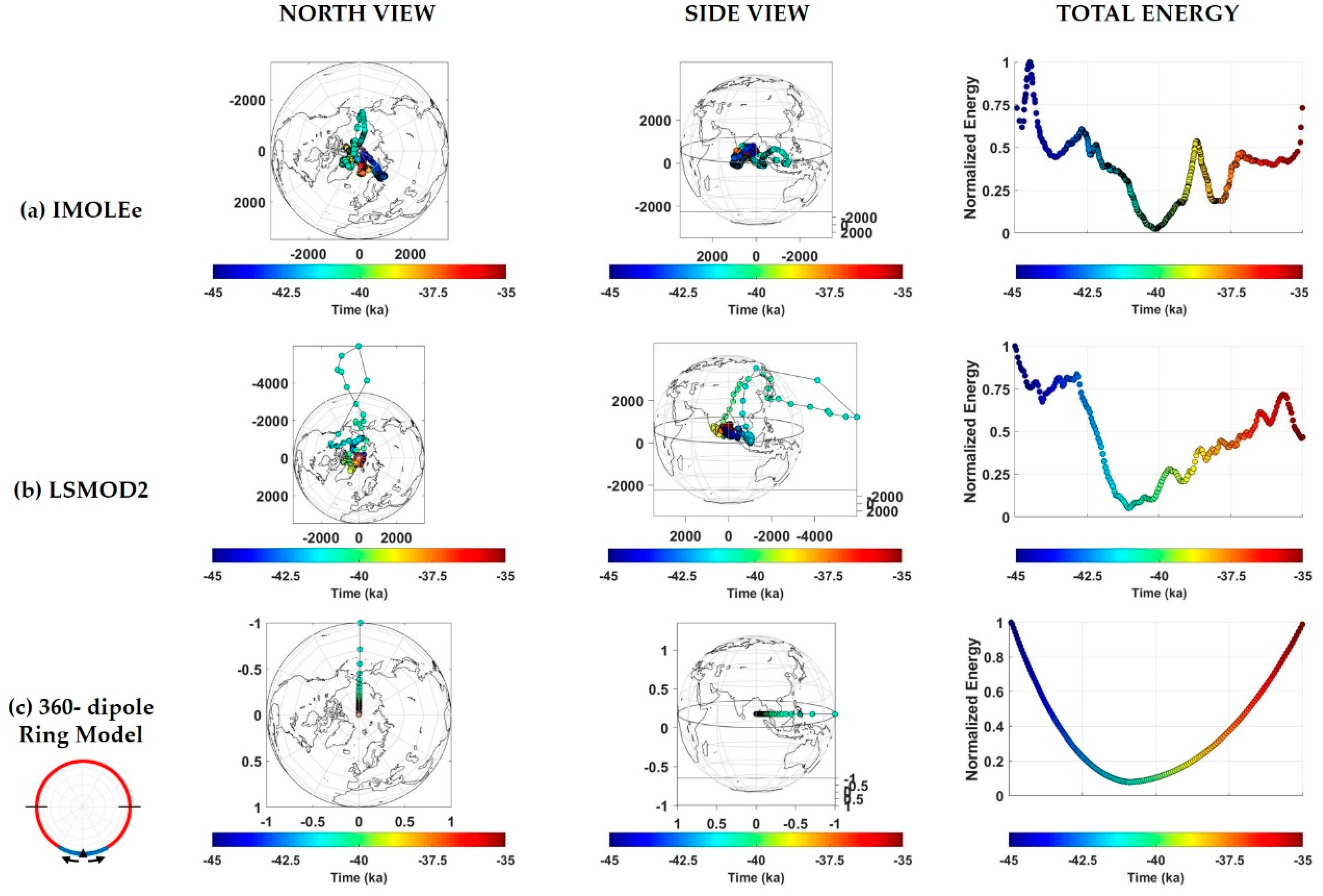
3.1. The Matuyama-Brunhes Transition

The evolution of the Earth’s magnetic field during the last reversal, the Matuyama-Brunhes 780 kyr ago, was analyzed from the IMMAB4 (up to its maximum degree 4). The location of the ED during the transition is shown in Figure 2a along with the normalized (dividing by the maximum value) total energy at the Earth’s surface calculated summing up the decomposition of the spatial power spectra at each epoch for each degree (following [34]):
R n = ( n + 1 ) m = 0 n ( g n m ) 2 + ( h n m ) 2
The departure of the ED from the Earth’s center starts at around 780 ka. The location of its center seems to follow a meridian plane (around 20° E) towards the Atlantic sector. The minimum of energy is reached at around 775 ka. Instabilities produced in the calculation process by higher harmonic degrees make the use of the ED approximation useless between 775.5–773.5 ka. The recovery of the field starts around 772 ka and it is displayed in Figure 2a as a return of the ED to the Earth’s center following the meridian plane of approximately 200° E. Regarding the Z-axis, when projecting the ED in the 20° E–200° E meridian, it seems to follow a linear path inclined around 23°, moving southwards at the beginning of the transition and coming back from the North Hemisphere in the recovering phase (side view, Figure 2a).
The apparent path followed by the ED is surprisingly very consistent: it is confined between 10° E–20° E meridians at the beginning of the transition and by the 190° E–200° E meridians during the recovering phase, which are sectors nearly symmetric with respect to the rotation axis. This simple behavior suggests us to model this transition with our 360-dipole ring model (360-DRM). Please note that, since we wanted to keep our model simple, we located the 360 dipoles at the equatorial plane, and thus we could not reproduce the ED movement in the Z-axis.
Displacement of the ED is in the opposite direction from the sector where the dipoles start to reverse (Figure 2b). That is, the displacement of the ED towards the Atlantic sector suggests that the reversal started in the Pacific Hemisphere. In this geometric context, we modeled the reversal by a simple ring model in which the dipole that reverses, at the first step, is the one located at 190° E. In the second step, the two neighboring dipoles also reverse, and so on. The procedure continues until the last dipole located at 10° E is reversed. To estimate the time duration of each step, i.e., the time between two consecutive reversed dipoles, we compared the normalized energy of the geomagnetic field at the Earth’s surface of both IMMAB4 paleoreconstruction and the 360-DRM. This provided a mean rate of 9 reversed dipoles per kyr for the beginning of the transition and a faster recovery of 18 reversed dipoles per kyr. The resulting evolution of the ED from the 360-DRM and the normalized energy at Earth’s surface are also shown in Figure 2b. Please note that the normalized total energy was calculated up to maximum degree 4 for both the IMMAB4 paleoreconstruction and the 360-DRM. It is worth noting that although the 360-DRM was generated up to degree 10, just the first 24 Gauss coefficients were significant, i.e., up to degree 4 (Figure S2).

3.2. The Laschamp Excursion

Two paleoreconstructions were used to study the Laschamp excursion: the IMOLEe and the LSMOD.2. The LSMOD.2 originally spans from 50 to 30 ka, but to homogenize we considered the same time interval that the IMOLEe, between 45 and 35 ka. Figure 3a,b show the evolution of the ED for both paleoreconstructions (following the same structure of Figure 2). A displacement of the ED towards 180° E near to the energy minimum (~41 ka) in both paleoreconstructions can be observed, although the departure from the Earth’s center is more limited in the case of the IMOLEe paleoreconstruction. The displacement of the ED is confined in the equatorial plane except for the period related to the energy minimum in the LSMOD.2 (between 41.5 ka and 40 ka).
Following the same approach as for the Matuyama-Brunhes transition, we adjusted the 360-DRM to recreate the evolution of the ED and the energy at the Earth’s surface (Figure 3c). The normalized total energy was calculated up to the maximum degree provided by the IMOLEe paleoreconstruction, which is n = 5, in the three cases (IMOLEe, LSMOD.2, and the 360-DRM).
Since excursions could be considered as aborted reversals (e.g., [4,8]), we started with the simplest model in which the reversed region is located at 0° E and spans up to 270° E and 90° E. That is, 180 dipoles are reversed (with a rate of 22 reversed dipoles per kyr) and then the reversal is aborted and the dipoles return to the original configuration (with 15 reversed dipoles per kyr). The 360-DRM reproduces the path of the ED along the 180° E meridian plane observed in the two paleoreconstructions and the general evolution of the energy at the Earth’s surface.
In terms of the total field energy, our model (Figure 3c) returned to the initial values at 35 ka, while the field energy given by the paleoreconstructions was not completely recovered at that time. This is probably related to the existence of the Mono Lake excursion (~34 ka). Since the LSMOD.2 spans from 50 to 30 ka, we also evaluated the path of the ED during this excursion (see Supplementary Material), identifying also a predominance of the ED location towards 180° E (Figure S3).

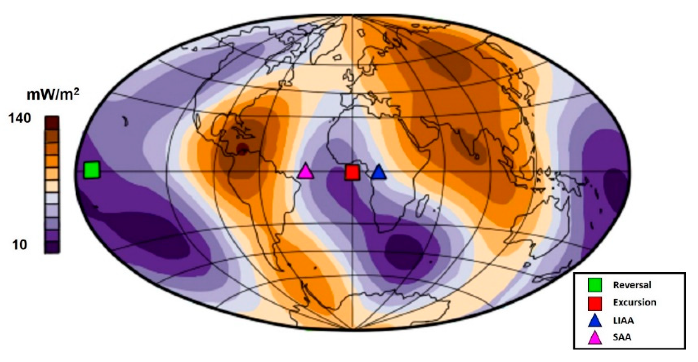
3.3. The Levantine Iron Age Anomaly (LIAA)

During the Iron Age, two intensity peaks of the geomagnetic field were recorded in the Levant region (between ~1050 BC and ~700 BC) known as the Levantine Iron Age Anomaly, LIAA [35,36]. This extreme anomalous event has been considered as a geomagnetic spike [35] and has attracted the attention of the geomagnetic community. A great number of studies have been published in the last decade on the LIAA extension and evolution (e.g., [37,38,39,40,41,42]).
Using the last global paleoreconstruction that spans this time interval, the SHAWQ-Iron Age, we estimated the location of the ED from 1300 BC to 0 (Figure 4a). It can be seen it moves from the Earth’s center towards the 20° E, reaching the greatest eccentricity around 1025 BC, and comes back to the origin following a meridian plane. For this time window, the vertical component of the ED is positive. That is, the ED departs toward the Northern Hemisphere, being its maximum distance to the Earth’s center at about 570 km. The normalized total energy, calculated up to maximum degree 10 for the SHAWQ-Iron Age, shows the two peaks in the intensity of the geomagnetic field at ~950 BC and ~775 BC, reflecting the characteristics of the LIAA. Please note that our ring model did not have enough resolution to reproduce in detail the two intensity peaks of the LIAA. Therefore, we considered only one intensity peak around 975 BC. In addition, considering the temporal limitation of the SHAWQ-Iron Age model, we do not believe that there is enough data to constrain the evolution of the LIAA in its earlier stages, so we focused on its final phase. Therefore, the 360-DRM was designed to catch the return to the center along the 20° E meridian, that is, to model the ED displacement at the end of the LIAA.
Since the effect of this anomaly is an increase in the intensity of the field in a localized region, in the 360-DRM we selected a sector of dipoles from 10° E to 30° E that increase their magnitude with 2 dipoles per 100 years increasing between 1300 BC and 950 BC and a rate of 1 changed dipole per 100 years in the recovery phase (between 950 BC and 0). In this case, the 360-DRM starts with several dipoles increased at 1300 BC since at that time the SHAWQ-Iron Age presents a normal flux patch (NFP) at the CMB according to Osete et al. [23]. The ED path from the 360-DRM seems to reproduce the recovery of the Earth’s magnetic field from the LIAA event. Please note that as a simple model with equatorial antisymmetry, our model was unable to reconstruct the details of the more complex ED displacement suggested by the SHAWQ-Iron Age, such as the displacement towards the Northern Hemisphere. Furthermore, the intensity of anomalous dipoles should only be considered qualitatively.

3.4. The South Atlantic Anomaly (SAA)

Probably the most important anomaly of the present-day geomagnetic field is the South Atlantic Anomaly (SAA), related to a low geomagnetic field intensity at the Earth’s surface spanning over the South Atlantic between the South American and African continents. Its emergence is linked to the presence of a reverse flux patch (RFP) at the CMB below Africa (e.g., [43,44]) around 1400 AD (although there are studies, such as [23,45], that suggest its presence at least since 950 AD) that migrated to the southwest during the following 500 years. Nowadays, the original RFP seems to be divided into two different patches: one below South America, which is vanishing, and another one in Africa, which is reinforcing [46]. The presence of this anomaly has been discussed as one of the main causes of the observed decay in the geomagnetic field intensity at a global scale (e.g., [47,48]), and even has been studied as a possible precursor of a geomagnetic polarity transition [49,50].
We analyzed the path followed by the ED from 700 AD to the present day (Figure 5a) by using the SHAWQ2k paleoreconstruction [23] until 1900 AD and then the IGRF-13 model [51]. At 700 AD the ED starts to move away from the Earth’s center westward and at 1100 AD turns to the Pacific sector. When the RFP is below southern Africa (~1200–1400 AD, [23]), the ED is found between 210° E and 230° E; later, when the RFP migrates westward throughout the South Atlantic, the ED moves eastward along the Pacific Hemisphere and it is located around 140° E at the present day (in 2020 AD, according to IGRF-13, a black star in Figure 5a). This observed evolution of the ED against the displacement of the SAA was also reported by Domingos et al. [52,53].
As our simple model is not capable of modeling in detail the two meridian planes followed by the ED associated with the evolution of the SAA, we chose to model the average migration of the ED. We consider that in each step of the 360-DRM two dipoles reverse (one for the first step) in the sector of 300° E–0° E, starting from the position 330° E. The rate of reversed dipoles is 5 per 100 years. The SHAQW2k and the 360-DRM presented consistent results in the decreasing trend of the total field energy for the last millennium (Figure 5, last column), although the decay in the ring model was slightly overestimated. The normalized total energy was calculated up to a maximum degree of 10 in both cases.

4. Discussion

Two types of anomalous events were studied in this work: extreme events related to polarity transitions (last reversal and excursions) and Holocene geomagnetic field anomalies (LIAA and SAA). The path followed by the ED during these events (Figure 6) seems to be constrained to a band around the 0°–180° E meridian (±30°). This apparently simple behavior is what inspired us to use de 360-DRM to model qualitatively the transitional paths and the Holocene anomalies.

4.1. Evolution of the Eccentric Dipole during the Last Millennia. Average Position and Characteristic Times

Olson and Deguen [54] studied the geomagnetic dipole eccentricity from geodynamo models trying to find out which of the boundary conditions control the eccentricity of the geomagnetic field: at the CMB or at the ICB. According to their simulation results, they concluded that lopsided inner core growth produces persistent eccentricity of the geomagnetic field, with the best-fitting dipole axis offset in the direction of fastest inner core solidification. Seismic anisotropy studies estimated the best fitting growth direction of the inner core from 120° E to 300° E, placing the regions of fastest and slowest growth under the Banda Sea (Indonesia) and Brazil, respectively [55].
When analyzing the historical archaeomagnetic and paleomagnetic models, Olson and Deguen [54] concluded that the eccentric dipole has moved into Earth’s Eastern Hemisphere over the past two centuries. In contrast, the average location of the ED for the last 10 kyr had an offset to the west according to CALS3k.4b [56] and CALS10k.1b [57] paleoreconstructions. Previously (last 5 Myr), it was located in the Eastern Hemisphere. From these results, they concluded that faster growth may have occurred in the Western Hemisphere of the inner core during the past ten millennia and that a reorientation of the location of the fastest inner core growth has occurred recently. A phenomenon that seems to have also occurred over the past 5 million years.
In Figure 6a, the ED paths and their time-average position are represented for the last reversal and last excursions studied in the Results section. The GGF100k paleoreconstruction that covers the last 100 kyr [58] is also plotted. It seems that transitional paths are constrained along the 0°–20° E/180°–200° E meridian.
Figure 6b shows the ED evolution in the equatorial plane during the Holocene according to different paleomagnetic reconstructions as well as its time-average location for the Holocene (SHA.DIF.14k [24] and CALS10k.2 [59]); for the Iron Age, the first millennium BC (SHAWQ-Iron Age [22]); and for the last 2 kyr (SHAWQ2k [23]). As expected, the mean position of the ED for a time window of 10 kyr was closer to the rotation axis than when studied for a shorter time window with the SHAWQ2k and the SHAWQ-Iron Age.
It must be also pointed out that although the average positions of the ED for the Holocene, calculated from CALS10k.2 and SHA.DIF.14k, did not differ by more than 170 km and were statistically indistinguishable, and the east-west hemisphere in which they are located was not the same. Both ED averages were in the North Hemisphere. Although it must be taken into account that the two paleoreconstructions are not based on the same type of data (thermoremanent in the case of the SHA.DIF.14k and including sedimentary data in CALS10k.2) and this could be the origin of the small discrepancy in the location of the ED mean position, it is perhaps more prudent to conclude that the paleomagnetic information is not yet accurate enough for the calculated ED averages to be significant (please note the error bars include in both cases the Earth’s center).
However, when using smaller time averages the eccentricity of the geomagnetic field is more evident. During the last 3 kyr the mean location of the ED moved from the European Hemisphere towards the Pacific Hemisphere biased by the presence of two major geomagnetic anomalies that occurred during this period: the LIAA and the SAA. The ED was located around 50° E and 300 km away from the Earth’s center during the first millennium BC according to the SHAWQ-Iron Age. The most eccentric position for the ED average was obtained during the last 2 millennia by SHAWQ2k paleoreconstruction: it was located at 330 km from the Earth’s center and deviated towards the Pacific Hemisphere, around 200° E meridian. It is important to note that SHAWQ2k and SHAWQ-Iron Age have a shorter time span than the SHA.DIF.14k and CALS10k.2, which affects the mean position of the ED. In both cases the mean position is biased by the presence of the anomalies.
González-López et al. [60] analyzed the secular variation at the millennial and centennial time scale searching for characteristic periods during the last 10 kyr by using different paleoreconstructions. They found characteristic times in the equatorial dipole and quadrupole terms (coefficients that control the equatorial location of the ED approximation) of around 1000–1400 years according to the SHA.DIF.14k, CALS10k.2, and SHAWQ2k paleoreconstructions. A wavelet analysis applied to the evolution of the ED as its distance from the Earth’s center (Rc), the distance from its equatorial projection to the Earth’s center (Sc), and the vertical displacement (Z) for the SHA.DIF.14, CALS10k.2, SHAWQ2k, and SHAWQ-Iron Age paleoreconstructions can be found in the Supplementary Material (Figure S4).
If the position of the ED is related to the anisotropy in the ICB as suggested by Olson and Deguen [54], these analyses would suggest that there are variations in the ICB conditions with characteristic periods of 500, 1000–1500, and 3000 years. Obviously, further investigations are needed to verify this fact.

4.2. The ED as an Indicator of Anomalous Regions at the CMB. Interpretation with the 360-DRM

Olson and Deguen [54] also modeled a lopsided ICB dynamo that spanned a dipole collapse event that resulted in a polarity change. Before the reversal, the dipole intensity was high, the dipole offset was relatively small, and the dipole axis was confined to the cold Hemisphere of the core. When the dipole collapsed, the transitional path followed by the ED in the simulation was not so clear as the ones we observed from the paleoreconstructions (Figure 2a, Figure 3a,b, Figure 4a, Figure 5a and Figure S3), but it seems that the ED drifted far into the opposite hemisphere during the transition and before the field assumed a more complex multipolar structure. Following the polarity change, the dipole intensity was recovered, the new polarity was stabilized and the dipole axis returned to the cold hemisphere.
One of the most striking results of this study is the coherence of the paths followed by the ED during the polarity transition and the excursions studied (Figure 2a, Figure 3a,b and Figure S3). These are located very close to the meridian 0° E–180° E. During the Matuyama-Brunhes transition, according to the 360-DRM, the dipole that started the reversal (changing from reversed to normal polarity) was located at 190° E meridian (Pacific Hemisphere), and during the last excursions the first dipole that reversed the polarity (from normal to reversed polarity) appeared in the opposite meridian (the 0° meridian, Atlantic Hemisphere).
It is important to note that reversed dipoles will originate anomalous flux patches at the CMB centered in the location where the first dipole reversed. Following the simple 360-DRM, these anomalous flux patches would grow more or less in situ until they cover the entire CMB and the reversal is stabilized. In the case of the excursion the region of abnormal flux grows to a certain point, stops growing, and subsequently vanishes.
Considering the evolution of the ED as reflecting the production and gathering of flux patches at the CMB within preferential hemispheres was already proposed by Gallet et al. [18]. They also related the archaeomagnetic jerks to episodes of maximum geomagnetic field hemispheric asymmetry (the most eccentric events). Part of our work also analyzed the most eccentric episodes that occurred in the last 3.5 kyr, which seem to be related to the evolution of the most important anomalies of the geomagnetic field: the LIAA and the SAA. The major difference between the two anomalies is the sign associated with each of them. While the SAA has been related with a set of reversing dipoles located in the Atlantic Hemisphere (Figure 5b), the LIAA has been associated with a set of anomalous high-moment dipoles (Figure 4b). It is important to note that the ED tends to move towards the region where the intensity of the Earth’s magnetic field is higher. That is, toward the anomalous region if the anomaly is in the sense of the present dipole field, as the LIAA, and towards the opposite hemisphere if the event is associated to reversing dipoles, as it is the case of the SAA. We cannot reproduce in detail the ED migration associated to these anomalies with our simple ring model. However, it is important to underline that the anomalous dipoles are restricted in both cases to one quadrant: between 200° E and 30° E, that is, the African-Atlantic region.
The search for observables that relate deviation from the GAD of the Earth’s magnetic field and its relation to the lateral variations in heat flux at the CMB has been an active topic of research (e.g., [61,62,63,64,65], among others). In this context, a simple approximation to the geomagnetic field, as the ED, can help to enhance the Earth’s magnetic field lateral asymmetries. Our result showed that ED paths during anomalous Holocene events or during polarity reversal or excursions correlate well to the regions where the heat flux is low (e.g., [66]), as evidenced in Figure 7.
If the equivalence between ring dipoles and outer core convective columns is considered [19], these results support that extreme geomagnetic events are controlled by the CMB thermal flux heterogeneities (e.g., [67,68], among others).
Large heat flux is expected to concentrate the geomagnetic field (e.g., [69]), and this could be envisaged as magnetic dipoles that are anchored in regions where heat flux is high. In contrast, the anchoring of the dipoles is less in the regions of low heat flux. During reversals or excursions, the magnetic field is destabilized in the regions of low heat flux. This causes, as the simple 360-DRM indicates, the ED location to move in the opposite direction to the region in which the inversion began.
Other more complex explanations have been proposed to interpret the extreme events of the Earth’s magnetic field ([68,70], among others). For example, Terra-Nova et al. [71] considered that low CMB heat flux leads to core fluid upwelling [72] which disperses the magnetic field and causes events like SAA. However, this type of mechanism would not explain the existence of spikes (as the LIAA).
In any case, the ED evolution provides valuable information about the regions where changes start in polarity transitions and the location of the sources of important anomalies of the geomagnetic field. Although it is important to remember that the 360-DRM does not try to reproduce the quantitative characteristics of the geomagnetic field, but the qualitative ones (in terms of field geometry).

5. Conclusions

The evolution of the eccentric dipole was analyzed during different extreme events of the geomagnetic field using paleoreconstructions: the last reversal (~780 ka), last excursions (~41 ka and ~34 ka), and two important Holocene anomalies: the Levantine Iron Age Anomaly (~1000 BC) and the South Atlantic Anomaly (analyzed from ~700 AD to present day).
We observed two different behaviors of the ED for the reversal and the excursion events. During the Matuyama-Brunhes transition, the evolution can be separated into two parts: before the change of polarity the ED moves towards the Atlantic sector between 0° E and 30° E; after the transition, it comes back to the Earth’s center at opposite longitudes, 180° E–200° E. However, during the Laschamp and Mono Lake excursions, the ED has its movement confined to a longitude frame around 180° E, before and after the energy minimum. Despite this difference, both reversal and excursions presented a coincidence in the meridian plane followed by the ED path (0°–180° E).
The two Holocene anomalies studied have different nature and origin, and these are reflected in the position of the ED. While the LIAA is related to a local enhancement of the geomagnetic field (reproduced by our simple 360-DRM as a local increase of the dipoles) and the ED moves towards the anomalous region, during the SAA, which is modeled with reversing dipoles, the ED moves opposite to the anomaly.
Despite its simplicity, the 360-DRM is able to reproduce the ED path based on the paleoreconstructions information. Following the approximation that the dipoles could be related to convective columns in the outer core of the Earth, our simple model suggests that last reversal, last excursions, and Holocene anomalies were originated in the CMB regions where the heat flux is low.

Supplementary Materials

The following are available online at https://www.mdpi.com/article/10.3390/geosciences11110438/s1, Figure S1: evolution of the eccentric dipole according to the 360-dipole ring model proposed in this work for studying the Matuyama-Brunhes transition (whole time interval); Figure S2: Power spectra of the Gauss coefficients obtained with the 360-dipole ring model in all cases of study; Figure S3: Evolution of the eccentric dipole and the normalized total energy for the Mono Lake excursion; Figure S4: Wavelet analysis for the time evolution of the eccentric dipole using paleoreconstructions that cover the last 10 kyr.

Author Contributions

Conceptualization, A.G.-L., M.L.O., S.A.C. and F.J.P.-C.; methodology, A.G.-L., M.L.O., S.A.C., A.M.-C., F.J.P.-C. and P.R.; software, A.M.-C., F.J.P.-C. and P.R.; validation, A.G.-L., S.A.C.; formal analysis A.G.-L., M.L.O. and S.A.C.; investigation, A.G.-L., M.L.O., S.A.C., A.M.-C., P.R. and F.J.P.-C.; resources, M.L.O. and F.J.P.-C.; data curation, S.A.C.; writing—original draft preparation, A.G.-L. and M.L.O.; writing—review and editing, S.A.C., A.M.-C., P.R. and F.J.P.-C.; visualization, A.G.-L., A.M.-C. and P.R.; supervision, M.L.O. and S.A.C.; project administration, A.G.-L., M.L.O. and S.A.C.; funding acquisition, M.L.O. All authors have read and agreed to the published version of the manuscript.

Funding

This research was funded by Spanish Ministry of Education (FPU17/03635) and Spanish Ministerio de Ciencia e Innovación (CGL2017-92285-EXP, CGL2017-87015-P, PID2020-117105RB-I00, PID2020-113316GB-I00). The APC was funded by the project PID2020-117105RB-I00 funded by the Spanish Ministerio de Ciencia e Innovación.

Data Availability Statement

Gauss coefficients for GGF100k, CALS10k.2, SHAWQ-Iron Age, and SHAWQ2k paleoreconstructions are publicly available in earthref.org/ERDA; LSMOD.2 coefficients can be found here: https://doi.org/10.5880/GFZ.2.3.2019.001 (accessed on 20 October 2021); SHA.DIF.14k is publicly available at http://pc213fis.fis.ucm.es/download.html (accessed on 20 October 2021); data from IMMAB4 and IMOLEe are available under request from the corresponding author.

Acknowledgments

AG-L and PR thank the Spanish Ministerio de Eduación y Formación Profesional (FPU17/03635 and FPU18/01567, respectively). SAC acknowledges the Juan de la Cierva Formación Program (FJC2018-037643-I), and AMC thanks the contract funding from CGL2017-92285-EXP funded by the Spanish Ministerio de Ciencia, Innovación y Universidades. Authors acknowledge the financial support from Spanish Ministry of Education (FPU17/03635) and Spanish Ministerio de Ciencia e Innovación (CGL2017-92285-EXP, CGL2017-87015-P, PID2020-117105RB-I00, PID2020-113316GB-I00). We are very grateful for the contribution from two anonymous reviewers and the academic editor of this journal that have helped us to improve this work.

Conflicts of Interest

The authors declare no conflict of interest. The funders had no role in the design of the study; in the collection, analyses, or interpretation of data; in the writing of the manuscript, or in the decision to publish the results.

References

  1. Merrill, R.; McElhinny, M.; McFadden, P. (Eds.) The Magnetic Field of the Earth: Paleomagnetism, the Core, and the Deep Mantle, 1st ed.; Academic Press: San Diego, CA, USA, 1996. [Google Scholar]
  2. Glatzmaiers, G.; Roberts, P. A three-dimensional self-consistent computer simulation of a geomagnetic field reversal. Nature 1995, 377, 203–209. [Google Scholar] [CrossRef]
  3. Amit, H.; Leonhardt, R.; Wicht, J. Polarity Reversals from Paleomagnetic Observations and Numerical Dynamo Simulations. Space Sci. Rev. 2010, 155, 293–335. [Google Scholar] [CrossRef]
  4. Cox, A.; Hillhouse, J.; Fuller, M. Paleomagnetic Records of Polarity Transitions, Excursions, and Secular Variation. Rev. Geophys. Space Phys. 1975, 13, 185–189. [Google Scholar] [CrossRef]
  5. Hoffman, K. Paleomagnetic Excursions, Abortive Reversals and Transitional Fields. Nature 1981, 294, 67–68. [Google Scholar] [CrossRef]
  6. Merrill, R.T.; McFadden, P.L. Geomagnetic field stability: Reversal events and excursions. Earth Planet. Sci. Lett. 1994, 121, 57–69. [Google Scholar] [CrossRef]
  7. Gubbins, G. The distinction between geomagnetic excursions and reversals. Geophys. J. Int. 1999, 137, F1–F3. [Google Scholar] [CrossRef] [Green Version]
  8. Valet, J.P.; Plenier, G.; Herrero-Bervera, E. Geomagnetic excursions reflect an aborted polarity state. Earth Planet. Sci. Lett. 2008, 274, 472–478. [Google Scholar] [CrossRef]
  9. Laj, C.; Mazaud, A.; Week, R. Geomagnetic reversal paths. Nature 1991, 351, 447. [Google Scholar] [CrossRef]
  10. Garnero, E.J.; Lay, T.; McNamara, A. Implications of lower-mantle structural heterogeneity for existence and nature of whole-mantle plumes. In Plates, Plumes, and Planetary Processes, 1st ed.; Foulger, G.R., Jurdy, D.M., Eds.; Geological Society of America: Boulder, CO, USA, 2007; Volume 430, pp. 79–101. [Google Scholar] [CrossRef] [Green Version]
  11. French, S.W.; Romanowicz, B.A. Whole-mantle radially anisotropic shear velocity structure from spectral-element waveform tomography. Geophys. J. Int. 2014, 199, 1303–1327. [Google Scholar] [CrossRef] [Green Version]
  12. Tric, E.; Laj, C.; Valet, J.P.; Tucholka, P.; Guichard, F. The Blake geomagnetic event: Transition geometry, dynamical characteristics and geomagnetic significance. Earth Planet. Sci. Lett. 1991, 102, 1–13. [Google Scholar] [CrossRef]
  13. Osete, M.L.; Martín-Chivelet, J.; Rossi, C.; Edwards, R.L.; Egli, R.; Muñoz-García, M.B.; Wang, X.; Pavón-Carrasco, F.J.; Heller, F. The Blake geomagnetic excursion recorded in a radiometrically dated speleothem. Earth Planet. Sci. Lett. 2012, 353–354, 173–181. [Google Scholar] [CrossRef] [Green Version]
  14. Leonhardt, R.; Fabian, K.; Winklhofer, M.; Ferk, A.; Laj, C.; Kissel, C. Geomagnetic field evolution during the Laschamp excursion. Earth Planet. Sci. Lett. 2009, 278, 87–95. [Google Scholar] [CrossRef]
  15. Langereis, C.G.; van Hoof, A.M.; Rochette, P. Longitudinal confinement of geomagnetic reversal paths as a possible sedimentary artefact. Nature 1992, 358, 226–230. [Google Scholar] [CrossRef]
  16. Valet, J.P.; Meynadier, L.; Quentin, S.; Thouveny, N. When and why sediments fails to record the geomagnetic field during polarity reversals. Earth Planet. Sci. Lett. 2016, 453, 96–107. [Google Scholar] [CrossRef]
  17. Nilsson, A.; Snowball, I.; Muscheler, R.; Uvo, C.B. Holocene geocentric dipole tilt model constrained by sedimentary paleomagnetic data. Geochem. Geophys. Geosyst. 2010, 11, Q08018. [Google Scholar] [CrossRef]
  18. Gallet, Y.; Hulot, G.; Chulliat, A.; Genevey, A. Geomagnetic field hemispheric asymmetry and archeomagnetic jerks. Earth Planet Sci. Lett. 2009, 284, 179–186. [Google Scholar] [CrossRef]
  19. Mori, N.; Schmitt, D.; Ferriz-Mas, A.; Wicht, J.; Mouri, H.; Nakamichi, A.; Morikawa, M. A domino model for geomagnetic field reversals. Phys. Rev. E 2013, 87, 012108. [Google Scholar] [CrossRef] [PubMed] [Green Version]
  20. Leonhardt, R.; Fabian, K. Paleomagnetic reconstruction of the global geomagnetic field evolution during the Matuyama/Brunhes transition: Iterative Bayesian inversion and independent verification. Earth Planet. Sci. Lett. 2007, 253, 172–195. [Google Scholar] [CrossRef]
  21. Korte, M.; Brown, M.; Panovska, S.; Wardiniski, I. Robust Characteristics of the Laschamp and Mono Lake Geomagnetic Excursions: Results from Global Field Models. Front. Earth Sci. 2019, 7, 86. [Google Scholar] [CrossRef] [Green Version]
  22. Osete, M.L.; Molina-Cardín, A.; Campuzano, S.A.; Aguilella-Arzo, G.; Barrachina-Ibáñez, A.; Falomir-Granell, F.; Oliver Foix, A.; Gómez-Paccard, M.; Martín-Hernández, F.; Palencia-Ortas, A.; et al. Two archaeomagnetic intensity maxima and rapid directional variation rates during the Early Iron Age observed at the Iberian coordinates. Implications on the evolution of the Levantine Iron Age Anomaly. Earth Planet. Sci. Lett. 2020, 533, 116047. [Google Scholar] [CrossRef]
  23. Campuzano, S.A.; Gómez-Paccard, M.; Pavón-Carrasco, F.J.; Osete, M.L. Emergence and evolution of the South Atlantic anomaly revealed by the new paleomagnetic reconstruction SHAWQ2k. Earth Planet. Sci. Lett. 2019, 512, 17–26. [Google Scholar] [CrossRef]
  24. Pavón-Carrasco, F.J.; Osete, M.L.; Torta, J.M.; De Santis, A. A geomagnetic field model for the Holocene based on archaeomagnetic and lava flow data. Earth Planet. Sci. Lett. 2014, 388, 98–109. [Google Scholar] [CrossRef]
  25. Schmidt, A. Der magnetische Mittlepunkt der Erde und seine Bedeutung. Gerl. Beitr. Geophys. 1934, 41, 346–358. [Google Scholar]
  26. Bartels, I. The eccentric dipole approximating the Earth’s magnetic field. Terr. Magn. Atmos. Electr. 1936, 41, 225–250. [Google Scholar] [CrossRef]
  27. Sano, Y. A best-fit eccentric dipole and the invariance of the Earth’s dipole moment. J. Geomag. Geoelectr. 1991, 43, 825–837. [Google Scholar] [CrossRef]
  28. Lowes, F.J. The geomagnetic eccentric dipole: Facts and fallacies. Geophys. J. Int. 1994, 118, 671–679. [Google Scholar] [CrossRef] [Green Version]
  29. Koochack, Z.; Fraser-Smith, A.C. An update on the centered and eccentric geomagnetic dipoles and their poles for the years 1980–2015. Earth Space Sci. 2017, 4, 626–636. [Google Scholar] [CrossRef] [Green Version]
  30. James, R.W.; Winch, D.E. The eccentric dipole. Pure Appl. Geophys. 1967, 66, 77–86. [Google Scholar] [CrossRef]
  31. Fraser-Smith, A.C. Centered and Eccentric Geomagnetic Dipoles and Their Poles, 1600–1985. Rev. Geophys. 1987, 25, 1–16. [Google Scholar] [CrossRef] [Green Version]
  32. Finlay, C.C. Earth’s eccentric magnetic field. Nat. Geosci. 2012, 5, 523–524. [Google Scholar] [CrossRef]
  33. Whaler, K.A.; Gubbins, D. Spherical harmonic analysis of the geomagnetic field: An example of a linear inverse problem. Geophys. J. R. Astron. Soc. 1981, 65, 645–693. [Google Scholar] [CrossRef] [Green Version]
  34. Lowes, F.J. Spatial Power Spectrum of the Main Geomagnetic Field, and Extrapolation to the Core. Geophys. J. R. Astr. Soc. 1974, 36, 717–730. [Google Scholar] [CrossRef]
  35. Ben-Yosef, E.; Tauxe, E.; Levy, T.E.; Shaar, R.; Ron, H.; Najjar, M. Geomagnetic intensity spike recorded in high resolution slag deposit in Southern Jordan. Earth Planet. Sci. Lett. 2009, 287, 529–539. [Google Scholar] [CrossRef]
  36. Shaar, R.; Ben-Yosef, E.; Tauxe, L.; Agnon, A.; Kessel, R. Geomagnetic field intensity: How high can it get? How fast can it change? Constraints from Iron Age copper slag. Earth Planet. Sci. Lett. 2011, 301, 297–306. [Google Scholar] [CrossRef]
  37. Di Chiara, A.; Tauxe, L.; Speranza, F. Paleointensity determination from São Miguel (Azores Archipielago) over the last 3 ka. Phys. Earth Planet. Inter. 2014, 234, 1–13. [Google Scholar] [CrossRef] [Green Version]
  38. De Groot, L.V.; Béguin, A.; Kosters, M.E.; van Rijsingen, E.M.; Struijk, E.L.; Biggin, A.J.; Hurst, E.A.; Langereis, C.G.; Dekkers, M.J. High paleointensities for the Canary Islands constrain the Levant geomagnetic high. Earth Planet. Sci. Lett. 2015, 419, 154–167. [Google Scholar] [CrossRef]
  39. Cai, S.; Jin, G.; Tauxe, L.; Deng, C.; Qin, H.; Pan, Y.; Zhu, R. Archaeointensity results spanning the past 6 kiloyears from eastern China and implications for extreme behaviors of the geomagnetic field. Proc. Natl. Acad. Sci. USA 2017, 114, 39–44. [Google Scholar] [CrossRef] [Green Version]
  40. Molina-Cardín, A.; Campuzano, S.A.; Osete, M.L.; Rivero-Montero, M.; Pavón-Carrasco, F.J.; Palencia-Ortas, A.; Martín-Hernández, F.; Gómez-Paccard, M.; Chauvin, A.; Guerrero-Suárez, S.; et al. Updated Iberian Archeomagnetic Catalogue: New Full Vector Paleosecular Variation Curve for the Last 3 Millenia. Geochem. Geophys., Goesyst. 2018, 19, 3637–3656. [Google Scholar] [CrossRef] [Green Version]
  41. Béguin, A.; Filippidi, A.; de Lange, G.J.; de Groot, L.V. The evolution of the Levantine Iron Age geomagnetic Anomaly captured in Mediterranean sediments. Earth Planet. Sci. Lett. 2019, 511, 55–66. [Google Scholar] [CrossRef]
  42. Rivero-Montero, M.; Gómez-Paccard, M.; Kondopoulou, D.; Tema, E.; Pavón-Carrasco, F.J.; Aidona, E.; Campuzano, S.A.; Molina-Cardín, A.; Osete, M.L.; Palencia-Ortas, A.; et al. Geomagnetic field intensity changes in the Central Mediterranean between 1500 BCE and 150 CE: Implications for the Levantine Iron Age Anomaly evolution. Earth Planet. Sci. Lett. 2021, 557, 116732. [Google Scholar] [CrossRef]
  43. Hulot, G.; Eymin, C.; Langlais, B.; Mandea, M.; Olsen, N. Small-scale structure of the geodynamo inferred from Oersted and Magsat satellite data. Nature 2002, 416, 620–623. [Google Scholar] [CrossRef]
  44. Olson, P.; Amit, H. Changes in earth’s dipole. Naturwissenschaften 2006, 93, 516–542. [Google Scholar] [CrossRef] [PubMed]
  45. Tarduno, J.A.; Watkeys, M.K.; Huffman, T.N.; Cottrell, R.D.; Blackman, E.G.; Wendt, A.; Scribner, C.A.; Wagner, C.L. Antiquity of the South Atlantic Anomaly and evidence for top-down control on the geodynamo. Nat. Commun. 2015, 6, 7865. [Google Scholar] [CrossRef] [PubMed] [Green Version]
  46. Pavón-Carrasco, F.J.; De Santis, A. The South Atlantic Anomaly: The Key for a Possible Geomagnetic Reversal. Front. Earth Sci. 2016, 4, 40. [Google Scholar] [CrossRef] [Green Version]
  47. Finlay, C.C.; Aubert, J.; Gillet, N. Gyre-driven decay of the Earth’s magnetic dipole. Nat. Commun. 2016, 7, 10422. [Google Scholar] [CrossRef] [Green Version]
  48. Terra-Nova, F.; Amit, H.; Hartmann, G.A.; Trindade, R.I.F.; Pinheiro, K.J. Relating the South Atlantic Anomaly and geomagnetic flux patches. Phys. Earth Planet. Inter. 2017, 266, 36–53. [Google Scholar] [CrossRef]
  49. De Santis, A.; Qamili, E.; Wu, L. Toward a possible next geomagnetic transition? Nat. Hazards Earth Syst. Sci. 2013, 13, 3395–3403. [Google Scholar] [CrossRef] [Green Version]
  50. Laj, C.; Kissel, C. An impeding geomagnetic transition? Hints from the past. Front. Earth Sci. 2015, 3, 61. [Google Scholar] [CrossRef] [Green Version]
  51. Alken, P.; Thébault, E.; Beggan, C.D.; Amit, H.; Aubert, J.; Baerenzung, J.; Bondar, T.N.; Brown, W.J.; Califf, S.; Chambodut, A.; et al. International Geomagnetic Reference Field: The thirteenth generation. Earth Planets Space 2021, 73, 49. [Google Scholar] [CrossRef]
  52. Domingos, J.; Jault, D.; Pais, M.A.; Mandea, M. The South Atlantic anomaly throughout the solar cycle. Earth Planet. Sci. Lett. 2017, 473, 154–163. [Google Scholar] [CrossRef] [Green Version]
  53. Domingos, J.; Pais, M.A.; Jault, D.; Mandea, M. Temporal resolution of internal magnetic field modes from satellite data. Earth Planets Space 2019, 71, 2. [Google Scholar] [CrossRef] [Green Version]
  54. Olson, P.; Deguen, R. Eccentricity of the geomagnetic dipole caused by lopsided inner core growth. Nat. Geosci. 2012, 5, 565–569. [Google Scholar] [CrossRef]
  55. Frost, D.A.; Lasbleis, M.; Chandler, B.; Romanowicz, B. Dynamic history of the inner core constrained by seismic anisotropy. Nat. Geosci. 2021, 14, 531–535. [Google Scholar] [CrossRef]
  56. Korte, M.; Constable, C.G. Improving geomagnetic field reconstructions for 0-3 ka. Phys. Earth Planet. Inter. 2011, 188, 247–259. [Google Scholar] [CrossRef] [Green Version]
  57. Korte, M.; Constable, C.G.; Donadini, F.; Holme, R. Reconstructing the Holocene geomagnetic field. Earth Planet. Sci. Lett. 2011, 312, 497–505. [Google Scholar] [CrossRef] [Green Version]
  58. Panovska, S.; Constable, C.C.; Korte, M. Extending Global Continuous Geomagnetic Field Reconstructions on Timescales Beyond Human Civilization. Geochem. Geophys. Geosyst. 2018, 19, 4757–4772. [Google Scholar] [CrossRef] [Green Version]
  59. Constable, C.; Korte, M.; Panovska, S. Persistent high paleosecular variation activity in southern hemisphere for at least 10,000 years. Earth Planet. Sci. Lett. 2016, 453, 78–86. [Google Scholar] [CrossRef] [Green Version]
  60. González-López, A.; Campuzano, S.A.; Molina-Cardín, A.; Pavón-Carrasco, F.J.; De Santis, A.; Osete, M.L. Characteristic periods of the paleosecular variation of the Earth’s magnetic field during the Holocene from global paleoreconstructions. Phys. Earth Planet. Inter. 2021, 312, 106656. [Google Scholar] [CrossRef]
  61. Olson, P. Mantle control of the geodynamo: Consequences of topdown regulation. Geochem. Geophys. Geosyst. 2016, 17, 1935–1956. [Google Scholar] [CrossRef] [Green Version]
  62. Bloxham, J.; Gubbins, D. Thermal core-mantle interactions. Nature 1987, 325, 511–513. [Google Scholar] [CrossRef]
  63. Bloxham, J.; Jackson, A. Fluid flow near the surface of the Earth’s outer core. Rev. Geophys. 1991, 29, 97–120. [Google Scholar] [CrossRef]
  64. Aubert, J.; Tarduno, J.A.; Johnson, C.L. Observations and Models of the Long-Term Evolution of the Earth’s Magnetic Field. Space Sci. Rev. 2010, 155, 337–370. [Google Scholar] [CrossRef]
  65. Ziegler, L.B.; Constable, C.G. Testing the geocentric axial dipole hypothesis using regional paleomagnetic intensity records from 0 to 300 ka. Earth Planet. Sci. Lett. 2015, 423, 48–56. [Google Scholar] [CrossRef]
  66. Hernlund, J.W.; McNamara, A.K. The Core–Mantle Boundary Region. In Treatise on Geophysics, 2nd ed.; Gerald Schubert, Ed.; Elsevier: Oxford, UK, 2015; Volume 7, pp. 461–519. [Google Scholar] [CrossRef]
  67. Aubert, J.; Finlay, C.C.; Fournier, A. Bottom-up control of geomagnetic secular variation by the Earth’s inner core. Nature 2013, 502, 219–223. [Google Scholar] [CrossRef] [Green Version]
  68. Takahashi, F.; Tsunakawa, H.; Matsushima, M.; Mochizuki, N.; Honkura, Y. Effects of thermally heterogeneous structure in the lowermost mantle on the geomagnetic field strength. Earth Planet. Sci. Lett. 2008, 272, 738–746. [Google Scholar] [CrossRef]
  69. Gubbins, D. Thermal core-mantle interacticions: Theory and observations. In Earth’s Core: Dynamics, Structure and Rotation; Dehant, V., Creager, K., Karato, S., Zatman, S., Eds.; AGU Geodynamics Series; American Geophysical Union: Washington, DC, USA, 2003; ISBN 9780875905334. [Google Scholar]
  70. Olson, P.; Christensen, U.R. The time averaged magnetic field in numerical dynamos with nonuniform boundary heat flow. Geophys. J. Int. 2002, 151, 809–823. [Google Scholar] [CrossRef] [Green Version]
  71. Terra-Nova, F.; Amit, H.; Choblet, G. referred locations of weak surface field in numerical dynamos with heterogeneous core–mantle boundary heat flux: Consequences for the South Atlantic Anomaly. Geophys. J. Int. 2019, 217, 1179–1199. [Google Scholar] [CrossRef] [Green Version]
  72. Mound, J.; Davies, C.; Rost, S.; Aurnou, J. Regional stratification at the top of Earth’s core due to core–mantle boundary heat flux variations. Nat. Geosci. 2019, 12, 575–580. [Google Scholar] [CrossRef] [Green Version]
Figure 1. Schematic representation of the 360-dipole ring model (360-DRM). (a) Distribution of the dipoles (white) close to the ICB (red). The CMB (magenta) and the Earth’s surface (yellow) are also shown. (b,c) Equivalence between the polarities of the dipoles with blue/red circumferences, which will be used in the following figures.
Geosciences 11 00438 g001
Figure 2. Evolution of the ED and the normalized total energy for the Matuyama-Brunhes polarity reversal according to (a) IMMAB4 paleoreconstruction (position in km); and (b) the 360-DRM proposed in this paper (see Materials and Methods section). Blue/red circumference indicates the first dipoles to change their polarity (black triangle) and the propagation directions (black arrows). Note that in (b) the evolution of the ED position is dimensionless and it is presented for a shorter time interval (the color scale is different) to remark the direction of the displacement. Also note that the ED is virtually coincident with the origin before and after the selected shorter period (see Figure S1). Coastlines are plotted only for longitude reference (note they are projected on a sphere of arbitrary radius).
Geosciences 11 00438 g002
Figure 3. Evolution of the ED and the normalized total energy for the Laschamp excursion according to (a) IMOLEe paleoreconstruction (position in km); (b) LSMOD.2 paleoreconstruction (position in km); and (c) the 360-DRM proposed in this paper. Blue/red circumference indicates the first dipoles to change their polarity (black triangle), the propagation directions (black arrows), and the limits of the reversing regions (black lines). Note that in (c) the evolution of the ED is dimensionless. Coastlines are plotted only for longitude reference (note they are projected on a sphere of arbitrary radius).
Geosciences 11 00438 g003
Figure 4. Evolution of the ED and the normalized total energy between 1300 BC and 0 according to (a) SHAWQ-Iron Age paleoreconstruction (position in km), and (b) the 360-DRM proposed in this paper, increasing by a factor of 5 the magnitude of the dipoles between 10° E and 30° E (see main text). Orange circumference indicates the first dipoles to increase their magnitude (black triangle), the propagation directions (black arrows), and the limits of the region (black lines). Note that in (b) the evolution of the ED is dimensionless. Coastlines are plotted only for longitude reference (note they are projected on a sphere of arbitrary radius).
Geosciences 11 00438 g004
Figure 5. Evolution of the ED and the normalized total energy for the South Atlantic Anomaly period according to (a) the SHAWQ2k paleoreconstruction (position in km) and (b) the 360-DRM proposed in this paper, reversing and multiplying of the dipoles between 300° E and 0° E. Gray and black stars correspond to the ED location at 2000 and 2020 AD, respectively, calculated with the IGRF-13. Orange/green circumference indicates the dipoles that change their polarity (the first one is marked with a black triangle), the propagation directions (black arrows), and the limits of the reversing regions (black lines). Note that in (b) the evolution of the ED is dimensionless. Coastlines are plotted only for longitude reference (note they are projected on a sphere of arbitrary radius).
Geosciences 11 00438 g005
Figure 6. Thin lines represent the geomagnetic eccentric dipole (ED) locations in the equatorial plane relative to Earth’s center (a) during the last reversal and excursions and for the last 100 kyr according to the IMMAB4 (blue), IMOLEe (orange), and LSMOD.2 (green), and GGF100k (purple) paleoreconstructions, respectively, and (b) during the Holocene according to SHADIF14k (red), CALS10k2 (green), SHAWQ2k (yellow), and SHAWQ-Iron Age (purple) paleoreconstructions. Triangles are the time-average location of the ED for each paleoreconstruction calculated as the mean position in each axis. X and Y correspond to the geocentric cartesian axes contained in the equatorial plane and pointing to 0° and 90° E longitude, respectively. Note the different scales between both figures. Coastlines are plotted only for longitude reference (note they are projected on a sphere of arbitrary radius).
Geosciences 11 00438 g006
Figure 7. Present-day CMB heat flux from a mantle Global Circulation Model. Icons indicate the longitude of the first dipole reversed (increased for LIAA) according to the 360-DRM for each event studied (see legend). Adapted from Olson [61].
Geosciences 11 00438 g007
Publisher’s Note: MDPI stays neutral with regard to jurisdictional claims in published maps and institutional affiliations.

