Review

A Call for More Snow Sampling

by
Steven R. Fassnacht
1,2,3
1
ESS-Watershed Science, Colorado State University, Fort Collins, CO 80523-1476, USA
2
Cooperative Institute for Research in the Atmosphere, Fort Collins, CO 80523-1375, USA
3
Natural Resources Ecology Laboratory, Fort Collins, CO 80523-1499, USA
Geosciences 2021, 11(11), 435; https://doi.org/10.3390/geosciences11110435
Submission received: 16 February 2021 / Revised: 30 July 2021 / Accepted: 18 October 2021 / Published: 21 October 2021
(This article belongs to the Special Issue Monitoring of the Seasonal Snow Cover)

Abstract

:
The snowpack is important for water resources, tourism, ecology, and the global energy budget. Over the past century, we have gone from point measurements of snow water equivalent (SWE) to estimate spring and summer runoff volumes, to remote sensing of various snowpack properties at continuously finer spatial and temporal resolutions, to various complexities of snowpack and hydrological modeling, to the current fusion of field data with remote sensing and modeling, all to improve our estimates of the snowpack and the subsequent runoff. However, we are still limited by the uncertainty induced by scaling from point field measurements to the area represented by remote sensing and modeling. This paper uses several examples of fine-resolution sampling to issue a call to snow hydrologists and other earth scientists to collect more data, or at least to thoroughly evaluate their sampling strategy for collecting ground-truth measurements. Recommendations are provided for different approaches to have more representative sampling, when at all possible, to collect at least a few more samples or data points.

1. Introduction—Estimating the Amount of Snow in the Pack

At the turn of the 20th century, James E. Church began measuring snow water equivalent (SWE) in the mountains above Reno Nevada in an attempt to estimate the runoff volumes in the Truckee River [1]. We continue to sample snowpack properties to forecast water resources in various parts of the world [2,3,4]. We also use these snow data to understand hydrological processes [5], climate dynamics [6,7], and the impacts that snow has on ecosystems [8,9]. Snow has a huge financial impact on the global economy, estimated in the order of trillions of dollars annually [10]. Thus, especially in the context of climate variability and change, there is an urgent need for accurate estimates of snow distribution, especially for SWE [11].
Various review papers provide in-depth summaries of snow research, including snow research in general [12] and representing SWE in hydrologic models [13]. Dozier et al. [11] present different methods to estimate SWE across a mountain range: spatial interpolation for station observations, remote sensing, numerical models, and combinations thereof. This combination is presented in a schematic by Sturm [12] and is the recommended way forward to understand what is actually occurring with the snowpack, especially at different scales [14]. We typically use field measurements to provide ground truth for remotely sensed estimates and to evaluate models. Data collected on the ground often represent a point, such as individual field measurements or station monitoring. Conversely, the resolution within large extent hydrological models, such as those covering 1000 or more km2 (e.g., Precipitation Runoff Modeling System or PRMS [15,16], Variable Infiltration Capacity or VIC [17,18]) or for daily resolution remote sensing (e.g., Moderate Resolution Imaging Spectroradiometer or MODIS optical imagery [19,20], passive microwave imagery [21,22]) is from 0.5 to 25 km. Yet, the question: “How good or representative are the ground-truth measurements?” always arises. The purpose of this paper is to issue a call for more ground-based sampling at various scales to better address this question. Specific examples are used to highlight this need.
Hydrologists want to estimate SWE [23] and the associated spatial and temporal variability, but other snowpack properties are also important [12] and have process [13] and measurement [14] scales. This paper uses six sample datasets (three of snow depth only, two of depth, SWE, and density, and one of SWE only) to highlight snow sampling issues and opportunities. The sampling and analysis methods used for the six examples are presented first.
The first example presents the differences between manual and remotely sensed snow depth measurements to illustrate that a direct comparison may not be useful. The second and third examples show fine resolution differences in depth, SWE, and density during accumulation and melt, respectively. The fourth and fifth examples illustrate additional depth measurements about operational measurement locations. The final example shows results from an agency-initiated intercomparison effort for measuring SWE. Finally, the discussion puts these examples into context and provides some sampling recommendations.

2. Sampling and Analysis Methods

2.1. Measurement Evaluations

The simplest way to compare different techniques is sampling the same location, such as remote sensing versus field measurements, or adjacent to one another for field measurements, assuming limited spatial variability [24]. Similarly, comparing measurements using the same sampling method at various distances can assess scales of variability [14]. This further introduces the question of how representative a specific sample is for an area [25,26,27]. There are also errors associated with sampling [24,28] that may be considered random or systematic [29]. Random errors, such as natural variability, landscape elements, or variability in meteorological conditions, are not be easily identified while systematic errors are a bias, such as due to instrumentation [24] or the influence of anthropogenic elements on meteorology. Some of the impacts of each error can be evaluated [29], such as using a Monte Carlo approach [30], which has been used to assess the influence of unknown and instrumentation uncertainty [31].
Semi-variograms are a tool to evaluate the spatial structure of an earth system property [32]. In the simplest form, it is a plot of semi-variance among all samples or measurements over a specific range of distances versus this distance. An example in linear space is the variance between all samples that are up to 2 m apart, then the semi-variance between all samples from 2 to 4 m apart, etc. Important properties of a semi-variogram are the distance at which variance no longer increases, called the correlation length or scale break, and the magnitude of the semi-variance beyond the correlation length, called the sill. For snow data, the slope of the variogram in log–log space up to the correlation length is a measure of the fractal dimension [14,33,34].
The shape of the semi-variograms derived from concurrent lidar and snow depth measurements are compared in the first example. The second example of snow accumulation illustrates random snowfall variability over the meter scale and likely systematic error of the 10 s of meters, while the third example illustrates mostly systematic shade-induced snowmelt differences over the centimeter scale. The differences shown in the fourth and fifth examples are mostly random, while the variations in the sixth examples are likely systematic due to differences in the composition of the measurement equipment.

2.2. Airborne LiDAR Snow Depth

Light distance and ranging, or LiDAR, uses light in the short-wave portion of the spectrum to estimate distance by sending out a beam of light and measuring the travel time [35]. Different wavelengths are used (532, 1064, 1550 nm) based on the measurement distance, power availability, and other requirements [36]. LiDAR can be in the form of a single beam of light or as a waveform that provides multiple returns and thus information on canopy structure as well as snow depth [36]. LiDAR measurements can be made at millimeter to meter horizontal resolution with terrestrial units [36,37], at 1 to 3 m resolution for airborne systems [36,38], and at 10 s of meters for satellite systems, specifically ICESat [39] and ICESat2 [40]. The stated vertical resolution of the LiDAR is millimeters but is typically in the range of 10–20 cm [36].
Since Hopkinson et al. [35] used the difference between snow-on and snow-off scans to estimate snow depth from airborne LiDAR, LiDAR has become an effective tool to measure snow depth [36]. It was added for the last intensive observation period (IOP4) of the NASA Cold Land Process Experiment (CLPX) in Northern Colorado in the western U.S. [41], and that dataset has been studied extensively [34,42,43]. Various studies have compared LiDAR-based snow depth estimates to manual depth probe measurements (see [44] for a summary). The errors associated with snow depth estimates from LiDAR are a function of the slope of the terrain, look angle (i.e., horizontal scanning terrestrial or vertical scanning from airborne and satellite), the horizontal resolution, and the nature of the snow-off surface [36]. A common problem is the presence of shrubs below the snowpack, which does not allow for an adequate measurement of the ground surface [36].

Data Used to Compare LiDAR Versus Probe Snow Depth Measurements

The CLPX LiDAR data collected in early April 2003 were used to measure snow depth in the first example. These measurements were compared to manual snow depth measurements for six 1 km2 intensive study areas (ISA) with > 300,000 LiDAR snow depth estimates [41] (see Figure 1a). Note that the data collected at three additional sites (ISAs) in North Park were not assessed due to the shallow snow depth (typically less than 50 cm) and known errors for shallow snowpack [25], and mixed LiDAR returns among shrub cover (e.g., Artemisia tridentata [45]). The spacing of the LiDAR data was about 1.5 m. The snow depth was estimated to the nearest centimeter [34], with a vertical accuracy of about 5 cm [41], depending on the slope [36].

2.3. Snow Depth Probe Measurements

Manual measurements of snow depth are easier and quicker than SWE measurements. A snow depth probe is essentially a ruler pointed at the end that is inserted vertically into the snowpack. These depth probes can be compact, such as for backcountry use, i.e., avalanche probes, or what is commonly used is an anodized aluminum probe with 1 cm increments [46]. Snow depth measurements for the first, fourth, and fifth datasets used the latter probe.

2.4. Fresh and Shallow Snow Depth, SWE and Density Measurements

Bulk SWE over the snowpack is manually measured by extracting a snow core and determining the mass or depth of water [1]. Many different samplers have been created to extract a core and measure the mass [24,47,48]. Almost any tube can be used for such sampling with proper care and acknowledging its limitations; this includes a stove pipe [49] or a plastic drainage pipe [50]. For sampling individual snowpack layers, a short metal tube sharpened at one end, often called a SIPRE (Snow, Ice, and Permafrost Research Establishment) tube [51], is often used, while for shallow fresh, snow (snow depth < 30 cm), a plastic SnowMetrics snow tube http://www.snowmetrics.com (accessed on 30 July 2021) can be used. Here, the latter was used to measure fresh snow. The 5.4 cm diameter SnowMetrics corer is rotated as it is inserted vertically into the snowpack. The depth is measured on the outside of the tube. Using a 10 cm wide scraper, the snow on one side of the snow tube is removed, and the scraper is inserted between the soil/ground surface and the tube. The tube is inverted and hung from a spring scale. The mass in millimeters of SWE is estimated from the spring scale. Snowpack density, compared to the density of water, is computed as the ratio of SWE to depth. The snow tube was used in examples two and three. If obvious layers can be identified in each of the snow cores extracted from the snow tube, the density of each of those layers can be estimated by isolating them from the remainder of the core.
Snow surface roughness can be measured with a snow roughness board and converted into data using various methods [52,53]. If the snow roughness board is inserted through to flat ground, as was the case in example three, snow depth data can be estimated at sub-millimeter resolution. A photograph of the snow surface contrasting the black roughness board was converted into X-Y coordinates as per the method described in Fassnacht et al. [53]. In the third example, a 123 cm long snow roughness board was used to estimate snow depth at a ~0.25 mm resolution
SWE can be estimated by extracting and weighing any area of snow; early efforts to evaluate snow pillows used this technique by removing all the snow on top of a snow pillow [54]. In the third example, a second roughness board was inserted parallel to the first at a 30 cm offset. All the snow was excavated in 8 to 14.5 cm increments based on approximate uniform snow depth along the trench.

Local-Scale Accumulation and Melt Measurements

If one goes outside and measures the snow, that measurement may not be representative [25,27], depending on where we go and what the meteorological conditions are. Typically, measurements are made at meteorological stations that have specific citing requirements or in an assumed natural or undisturbed setting. However, this does not stop us from going outside of our homes and measuring the snow, even if it is while we are shoveling the sidewalk. As such, one simple experiment was performed to evaluate 1 to 10 m differences in accumulation versus the station measurements across town (a kilometer away). Another simple experiment evaluates differences in melt over the centimeter scale. While these two examples may not be realistic, they are meant to illustrate random and systematic errors.
Fresh snow accumulation was measured after a 20 to 30 cm snowfall event on 26 October 2020 in Fort Collins Colorado USA. Using the SnowMetrics tube on a grass surface, snow depth and SWE were measured, from which density was estimated, with samples in close proximity of one another; replicates were taken about 1 m apart and repeated about 10 m from one another on each of the north, east, south, and west side of the author’s house. These were compared to measurements 2.4 km away at two National Weather Service (NWS) stations https://www.ncdc.noaa.gov (accessed on 30 July 2021). The two NWS stations were about 10 m from one another.
A different snowfall event on 16 April 2020 produced 20 to 30 cm of fresh snow depth in Fort Collins. The next day was sunny with a maximum incoming short-wave radiation of almost 1000 W/m2, measured at FTC http://ccc.atmos.colostate.edu/~autowx/ (accessed on 30 July 2021). Just after solar noon on the following day (18 April), the author noticed irregular melt patterns due to partial shading from an overhead obstruction. Using the SnowMetrics tube, the author extracted cores at 11 locations and dug a trench between two snow roughness boards to depth and SWE. Density was computed per core or increment along the trench. Obvious layers were identified in each of the snow cores extracted from the snow tube; within the core, as each layer was removed, the remaining depth was estimated and remaining mass or SWE was measured. The density was estimated for each layer from SWE divided by depth by subtracting the measurements after removal of the layer from the measurements prior to removal of the layer. A photograph of the full inserted snow roughness board provided depth estimates to the nearest 0.25 mm [53].
Figure 1. (a) Mean and standard deviation (whiskers) snow depth derived from airborne LiDAR scans (data from [41]) and manual snow depth probe measurements (data from [46]) across six 1 km2 intensive study areas (ISA) in early April 2003 from the NASA Cold Land Process Experiment. The LiDAR-based depth estimates are from differentiating snow-on versus snow-off scans. The “all-LiDAR” dataset includes all depth estimates within each ISA (>300,000 samples). The mean difference between the snow depth probe and LiDAR estimates are presented above the bars for all matching points (teal) and the first points only (orange in italics). (b) There are 680 depth probe measurements per ISA with 100 being the first depth probe point (see Elder et al. [46]).
Geosciences 11 00435 g001

2.5. Operational Measurement

The operational snow course data include depth, SWE, and density. Such measurements are made using a variety of samplers e.g., [24] in countries that have seasonal snowpacks. In the United States, these data are collected by the Natural Resources Conservation Service (NRCS) https://www.wcc.nrcs.usda.gov/ (accessed on 30 July 2021) with a Federal Sampler [1,55], and the data are available through the National Water and Climate Center of the U.S. Department of Agriculture.
Globally, automated monitoring has been less extensive, with automated weather stations including sonic snow depth sensors [56]. More recently, SWE has been measured with a snow scale https://sommer.at/ (accessed on 30 July 2021) or through the attenuation of gamma radiation by the snowpack emitted from potassium and thallium in the earth <https://campbellsci.com/>. Snow pillows are used in some locations e.g., [57], but are only used operationally in the United States. There, the NRCS has been operating the automated snow telemetry (SNOTEL) network since the late 1970s [58]. These stations originally monitored SWE and cumulative precipitation and now also monitor air temperature and snow depth. SWE is measured using a snow pillow [59,60], while depth is measured using an ultrasonic depth sensor [56]. Snow course and SNOTEL depth measurements are used in examples four and five, and SNOTEL SWE data are used in example six. In the last example, the accumulation and melt patterns were compared for different materials used in the construction of the snow pillow. Currently, the standard snow pillow is black with a surface mesh; a tan/grey snow pillow and a black snow pillow each with a chain-link fence covering were also tested.

3. Sampling Examples

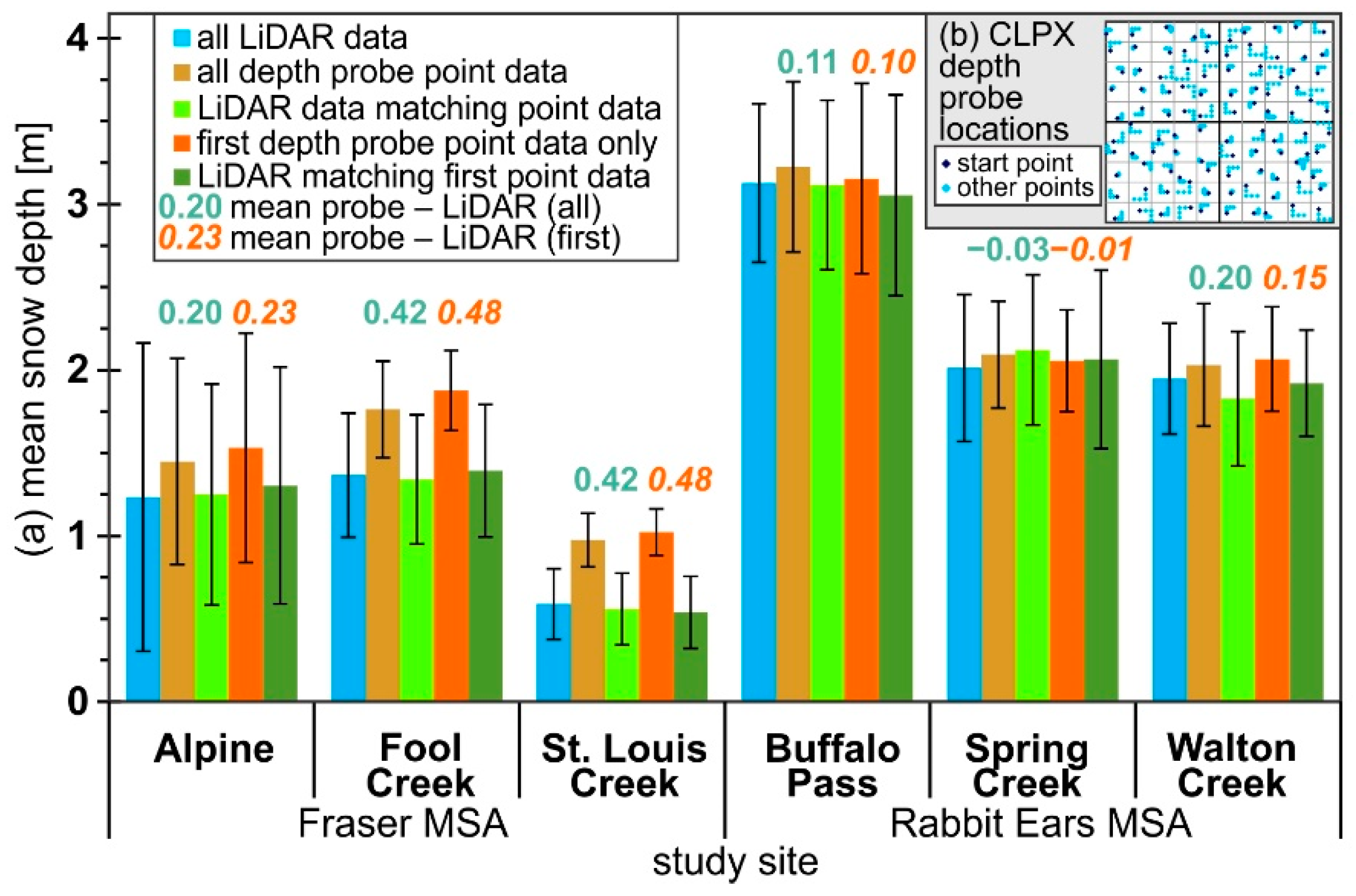
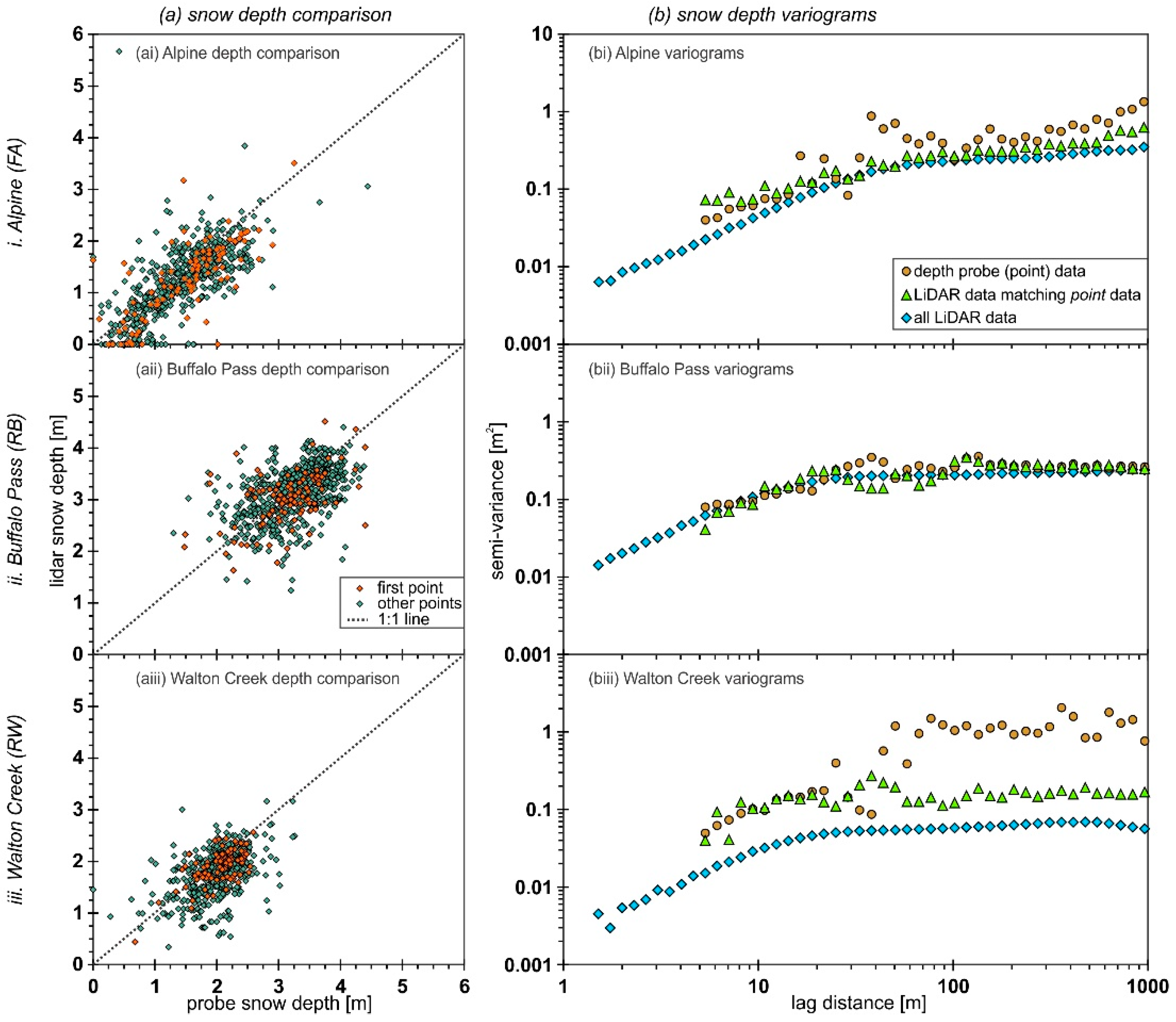
3.1. Airborne LiDAR versus Snow Depth Probe Data

There are up to 680 manual snow depth probe measurements [46]. All 680 measurements were only taken at the Buffalo Pass locations, with nine missing at Spring Creek (Figure 1). The random stratified sampling survey design was composed of ninety-six 100 × 100 m squares with five depth measurements randomly spaced 5, 10, 15, 20 or 25 m apart in an “L” and four squares with 50 measurements in an “L” spaced 1 m apart (Figure 1b) [46]. In the field, the initial manual depth probe measurement location (dark blue diamond in Figure 1b) was identified with a semi-permanent PVC pole. This pole was located with a hand-held GPS unit. Occasionally, the pole could not be found, and its location was estimated by GPS; the stated GPS error was typically 3 to 5 m, and the author found 5 to 10% of the poles to be missing during the IOP4 survey. The location of the other four measurements was based on the implementation by each snow surveyor, i.e., what the snow surveyor did in the field. The author was in the field for this survey and used the depth probe to measure the horizontal distance between measurement locations with the pre-specified direction being taken using a compass. It is assumed that the probes were inserted vertically into the snowpack just to the ground.
A direct comparison of point snow depth measurements to LiDAR-based depth estimates (Figure 2a) is not recommended [34,61,62] due to the inaccuracy of locating each measurement [36] and the scale difference [14]. The two issues with locating the measurements are the reported and the actual location differences. Relating to the former, the average difference in the location between the reported manual measurement and center of the LiDAR return was 83 cm, ranging from 0 to 395 cm. However, the locations of the manual measurements were reported to the nearest meter and the LiDAR to the nearest centimeter. Relating to the latter, an assessment of concurrent aerial photography illustrated that the location of these four points could deviate from their survey design [63]. From trigonometry, the depth probe point is 5% off from the assumed location for every degree that the bearing is off from true north (east, south, or west, from Figure 1b). For example, if the declination was not considered, ~10° E for CLPX sites in northern Colorado, then with a measurement interval of 25 m, the final depth probe point would be about 12.3 m from the assumed location. With a LiDAR resolution of ~1.5 m, then the depth probe measurement could be eight LiDAR pixels from where it should be. However, even comparing only the first point, which should be within one LiDAR pixel, the mean snow depth had a similar difference between the two datasets (Figure 1a). In fact, at the three Fraser MSA sites, the difference of probe minus LiDAR snow depth was 0.03 to 0.06 m greater when only comparing the first points.
The mean snow depth from all hundreds of thousands of LiDAR estimates was less than the manual snow depth probe measurements (blue- vs. gold-colored bars in Figure 1a). With the exception of Spring Creek (RS), the mean snow depth for all depth probe points was greater than the coincident LiDAR estimate (gold- vs. lime-colored bars in Figure 1a). The spatial structure of the distributed snow depth measurements can be seen from semi-variograms; the three ISAs (Alpine, Buffalo Pass, Walton Creek) evaluated by Deems et al. [34,64] are presented here (Figure 2b). The semi-variance across the range of lag distances was the same for the three datasets at Buffalo Pass (Figure 2bii), similar for both LiDAR datasets at Alpine (Figure 2bi), but different for the three datasets at Walton Creek (Figure 2biii). The Fool Creek, St. Louis Creek, and Spring Creek variograms (not shown) had similar patterns to Alpine with all LiDAR and LiDAR-matching points being essentially the same, with larger semi-variance for the point measurements at lag distances greater than the scale break.
There is noise, illustrated as variability with lag distance, in the depth probe semi-variograms, as also seen by Erxleben et al. [65] for Fool Creek. The semi-variograms for the LiDAR matching point data are less noisy than the depth probe semi-variograms, but not as smooth as the all LiDAR data (Figure 2b). This is due in part to the number of data points; there are 100 s of points collected from the depth probe versus 100,000 s of points collected from the airborne LiDAR survey. Similar scale breaks could be extracted from the three datasets for the Alpine and Buffalo Pass ISAs, since the datasets with fewer points still represent the snowpack, in comparison to the complete LiDAR dataset [66]. However, for the other for ISAs (Walton Creek shown in Figure 2biii), it is difficult to determine the scale break for the depth probe semi-variograms. The horizontal uncertainty and lack of data make it more difficult to assess spatial structure using depth probe measurements.
Since the average difference is between −0.03 and 0.48 m (Figure 1a), over-probing, while known to over-measure (over-probe) snow depth in the order of 5 cm due to penetration into the soil below the snow [28], is likely not the cause of these differences. The largest differences of 0.42 (all) and 0.48 (first point only) are at Fool Creek and St. Louis Creek, which had the densest forest canopy [34,43]. The Alpine ISA is divided into forest in the northwest and alpine in the southeast; however, there, the results were mixed with mean depth probe LiDAR difference for all points (first points only) was 0.26 (0.30) m for the open alpine terrain and 0.20 (0.36) m in the forest.

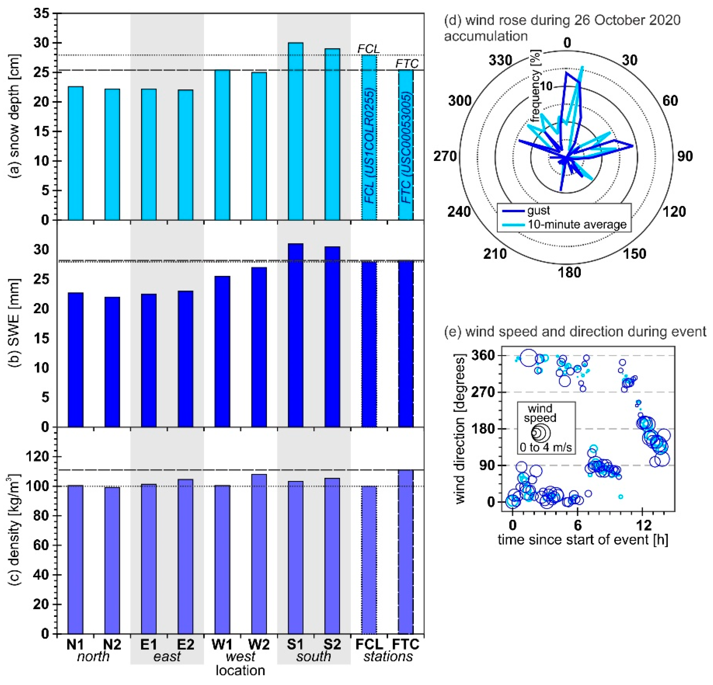
3.2. Fine Resolution Accumulation Differences

The two NWS stations reported 25 to 28 cm of accumulation over the 26 October 2020 Fort Collins snow storm (Figure 3a) based on twice-daily snowpack measurements [56]. While the two NWS measurements were only 10 m apart, there was a 10% difference in snow depth (Figure 3a). The around-the-house samples varied by 30% (north vs. south) (Figure 3a), while difference between locations (e.g., N1 vs. N2) was 1 cm or less. Around the house, spatial variability in SWE (Figure 3b) showed the same patterns as snow depth (Table S1), but the NWS SWE estimates were only 1% different from one another. The maximum difference in bulk density was about 10% around the house, and also 10% between the two NWS stations (Figure 3c).
The four locations around the house are within 10 m of the house, and W, S, and E are within 5 m of a fence or hedge, and it is assumed that there is similar shelter from wind. Over the course of the snowfall event, the wind blew from almost all directions (Figure 3d). Wind caused limited to no redistribution as the maximum 10 min (gust) wind speed at NWS station FTC was 2.64 (3.89) m/s with a mean 10 min (gust) wind speed of 1.13 (2.23) m/s (Figure 3e), but likely influenced accumulation patterns. Snow depth measurements during other snowfall events have not shown the same north-to-south difference (Figure 3).
One difference between the two NWS station snowpack estimates is due to precision and methodology. FTC is the official NWS COOP station, while FCL is the CoCoRaHS (Community Collaborative Rain, Hail and Snow Network https://www.cocorahs.org/ (accessed on 30 July 2021) station that is at the FTC weather station, so the measurements are within 10 m of one another. The FTC snow depth precision is 2.54 cm (1″), based on the COOP data entry system, while the FCL precision is 0.254 cm (0.1″) based on the CoCoRaHS data entry system. NWS snow depth was taken as snow on the ground (SNWD) rather than snowfall (SNOW) [Ryan et al., 56; 2008], in order to compare the NWS measurements to the around-the-house snow cores. At the FCL station, SWE was measured as SWE on the ground (WESD) to the nearest 2.54 mm (0.1″). However, for the FTC station, there were no such measurements, and cumulative precipitation was used to estimate SWE, as per Meinhardt and Fassnacht [67].

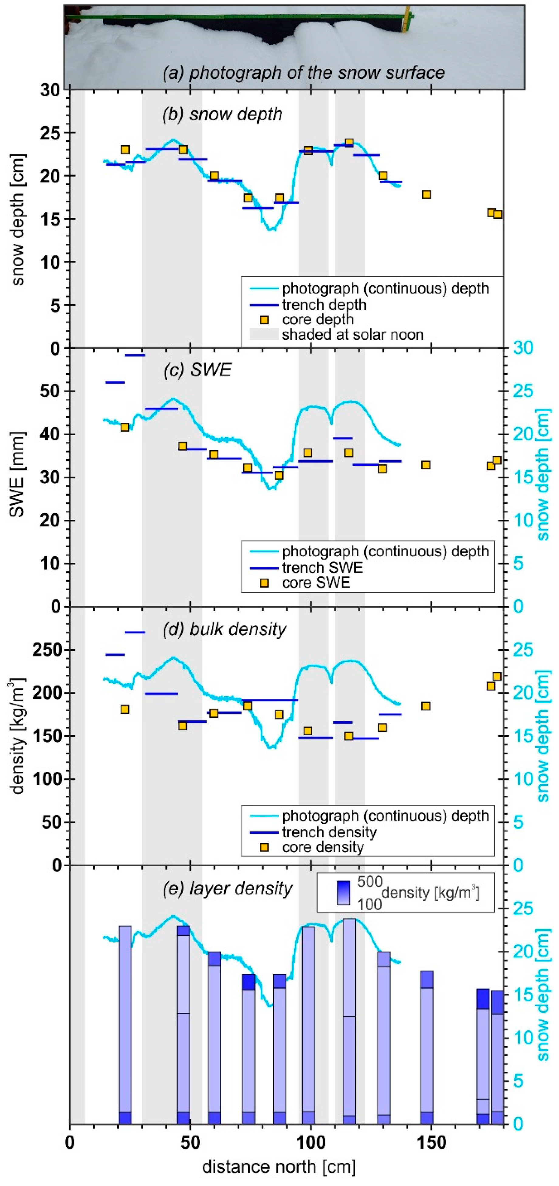
3.3. Fine Resolution Snowmelt Differences

From 00:00 to about 12:00 on 16 April 2020, an average of 26.3 cm of fresh snow fell at the author’s house, as measured at five locations on the north side using the SnowMetrics snowboard tube. This snowfall yielded about 29.6 mm of SWE and an average density of 112 kg/m3. Two days later, there was differential snowpack compaction and melt along the 180 cm transect (Figure 4). A snowboard (Figure 4a) was used to estimate continuous (~0.25 mm resolution) snow depth (Figure 4b and cyan-colored lines in Figure 4c,d). Snow cores (orange-colored squares in Figure 4b–d and Table S2a,b) were extracted at 11 locations, and the trench (blue-colored lines in Figure 4b–d) was dug to estimate depth (Figure 4b), SWE (Figure 4c), and density (Figure 4d). Obvious layers were identified in each of the snow cores extracted from the snow tube, and the density of each of those layers was estimated (Figure 4e).
The surface illustrated the areas with preferential melt and thus decreased SWE (distances > 50 cm; Figure 4c and Figure S1), as well as increased densification where the depth was the shallowest (distances from 70 to 90 cm and beyond 140 cm; Figure 4d–e). The snowpack changes are driven by short-wave radiation, with solar-noon shading (Figure 4b) over the areas with the least changes in the snowpack (Figure 4e). In each of the 11 cores, the bottom 1 to 1.5 cm was a refrozen layer (mean density of 332 kg/m3) and was thus easy to identify. The four cores from 50 to 90 cm and the three cores beyond 140 cm all received more solar loading and had meltwater at the top ~2 cm with a mean density of 372 kg/m3 (Figure 4e). The rest of the snowpack had a density of about 150 kg/m3.

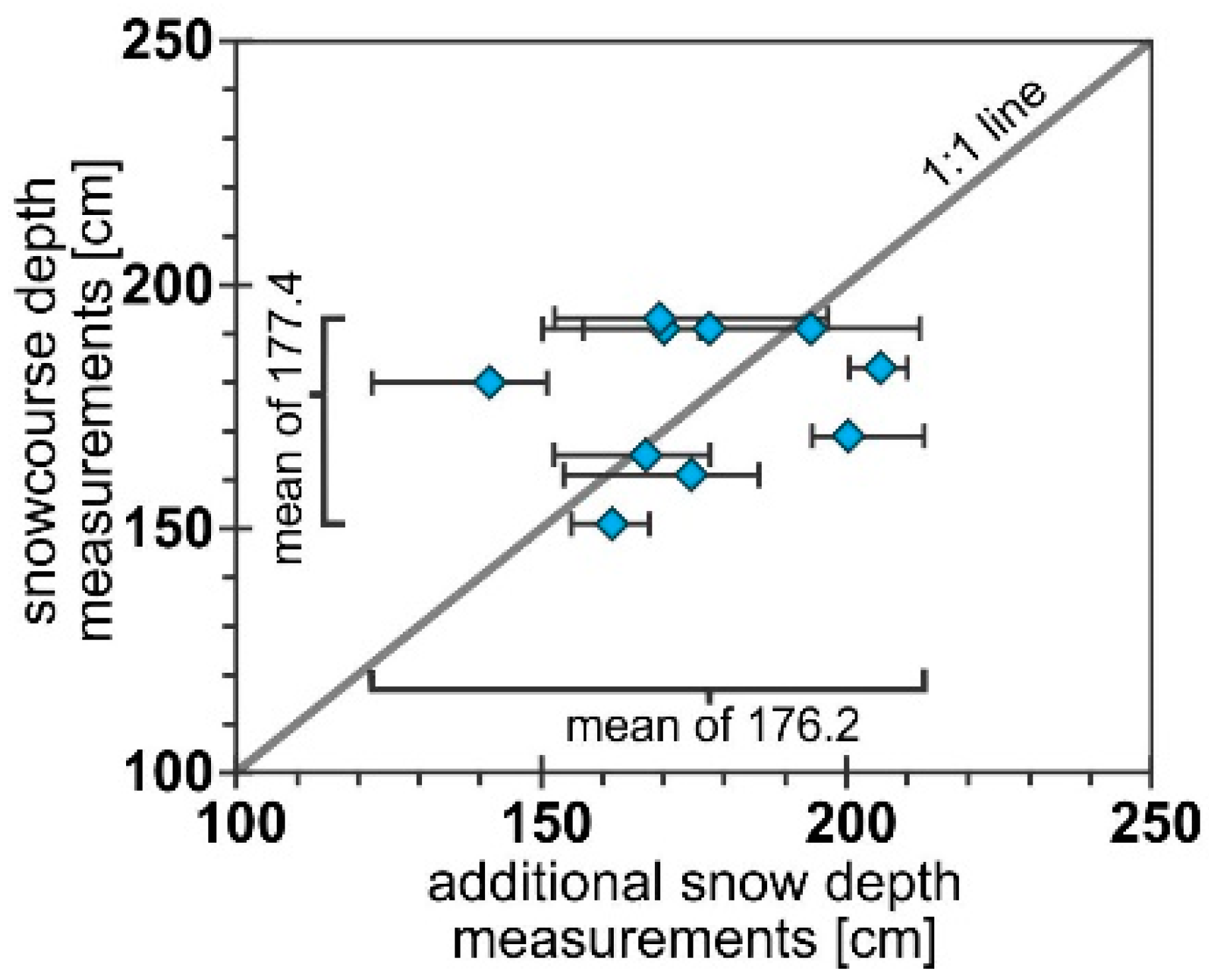
3.4. Additional Snow Depth Measurements around Operational Stations

To evaluate snow depth variability over short distances, five additional snow depth measurements were taken near each of the 10 individual Federal Sampler measurement locations at the NRCS Cameron Pass (station 05J01) snow course in Northern Colorado (Figure 5). There is variability among the individual snow course measurements themselves [68,69], and around each individual measurement (Figure 5). The mean snow depth along the snow course was only 1.2 cm different for the two methods (177.4 vs. 176.2 cm for the snowcourse vs. additional measurements, respectively), but the variability from the depth probe measurements was greater (Figure 5).
Twenty-four additional snow depth measurements were taken on two dates (2 and 4 June 2011) at 1, 2, and 3 m intervals in eight directions around the NRCS Joe Wright SNOTEL snow pillow in Northern Colorado to compare to the Judd ultrasonic snow depth sensor measurements of depth above the snow pillow [56] (Figure 6). The snowpack was melting, so the depth measurements taken on 2 June left holes in the snowpack (except for one of the 24 locations; Figure 6) that remained on 4 June, and thus depth was measured in the exact same location for the two dates. Snow depth varied but not systematically with direction or distance from the edge of the snow pillow (Figure 6a,b). Depth decreased at all but two locations, and on average it matched what was observed at the SNOTEL station (Figure 6c). However, the decrease was not uniform.

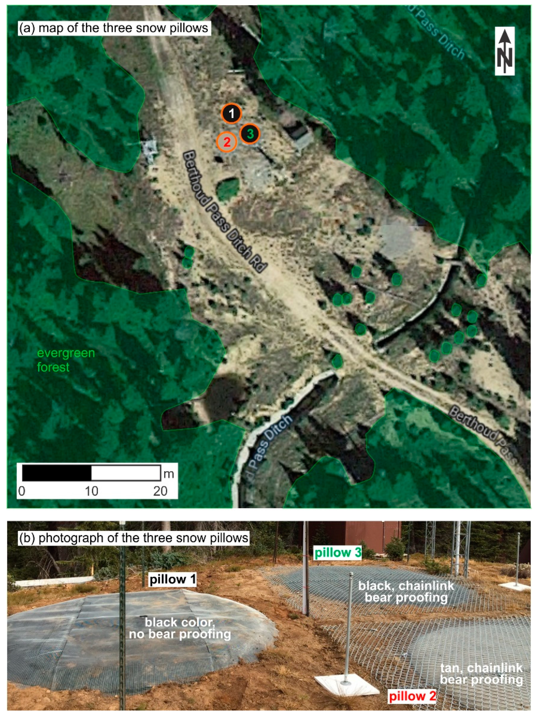
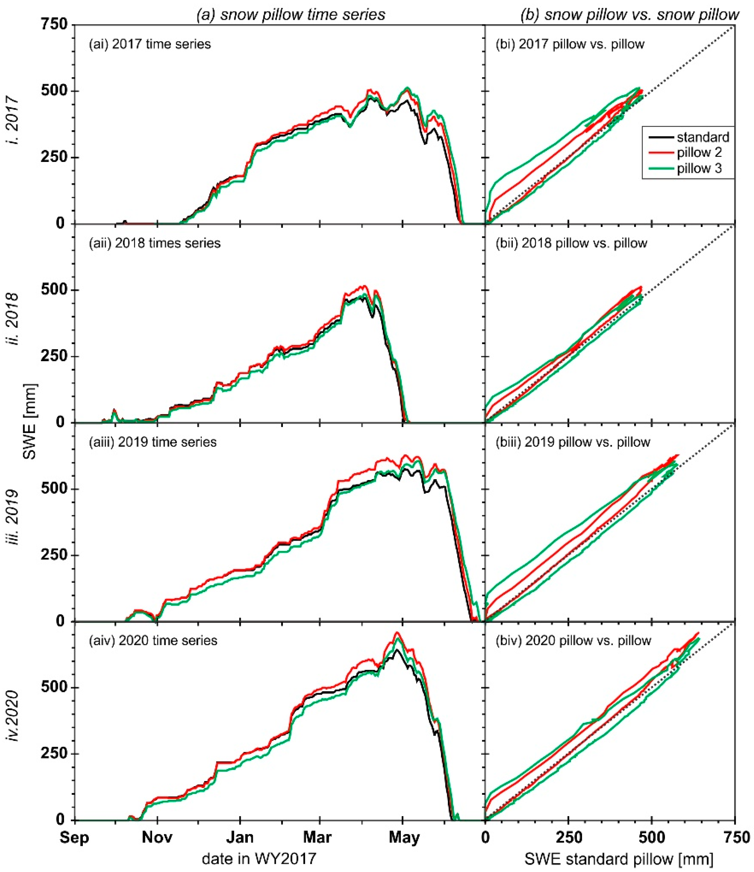
3.5. Sensor Comparisons

Sensors need to be evaluated; the difference between each measurement is a function of the sensor and spatial variability. At four locations across the domain of the NRCS Colorado Snow Survey office, additional snow pillows (and other sensors) have been installed to evaluate how snow pillow characteristics influence the measurement of SWE [70]. Four winters of data https://www.wcc.nrcs.usda.gov/ (accessed on 30 July 2021) from the Berthoud Summit SNOTEL station (station 05K14S/335) illustrate that the three pillows do not measure exactly the same SWE (Figure 7a), yet the differences are consistent from year to year (Figure 7b). Accumulation patterns are different among pillows; specifically, pillow 2 begins to accumulate more SWE than the standard pillow starting in February, while pillow 3 accumulates less snow by up to 30 mm (Figure 7b) after there is 50 mm on the ground but then in March starts to accumulate more than the standard pillow. Peak SWE at pillow 2 (pillow 3) is 33 to 66 (15 to 46) mm greater than the standard pillow. Pillow 3 melts out more slowly than the other two pillows (highest lines in Figure 7b), with a maximum difference of 125 mm in 2017 (Figure 7bi). However, while pillows 2 and 3 have more snow to melt than the standard pillow, the melt-out date is only two days earlier, except in 2018, when it is five days earlier.
SNOTEL stations are typically situated in forest clearings [71], in order to not be influenced by canopy interception and to decrease wind. The pillows are about 3.5 m in diameter and were placed about 2 m apart (Figure 8a,b). There are no trees from the southwest to the southeast for at least 20 m. At this site (Figure 8a), the forest does not throw shade differentially on any one of the snow pillows.
The expectation is that differences in snow pillow materials caused a difference in accumulation and melt (Domonkos 2016 [70]). The standard snow pillow is now black with a surface mesh (pillow 1 in Figure 2b). A tan/grey pillow is also available (pillow 2 in Figure 8b), and a chain-link fence covering yields a different surface roughness (pillows 2 and 3 in Figure 8b). It is assumed that the energy balance of the three snow pillows is different when the snowpack is shallow due to their color, i.e., albedo, and thus short-wave radiation associated with light penetration. Thus, material-related SWE variation should only be expected during the initial accumulation (depth less than 50 cm and SWE < 100 mm) and then during melt (likely shallower depth due to a decrease in light penetration from increased density).
The properties of the surface material could also influence the sensible and latent heat fluxes during initial accumulation, and these could cause differential melt. We assume that this would result in differences in SWE. However, we do not see differences in SWE until a certain amount of accumulation. Then, the differences can be 5% or greater (Figure 8b). Snow depth is not measured. It is possible that SWE is not initially different, but metamorphism rates may be different. This could cause densification at the non-standard pillows, yielding a lower snow depth. The “relative” depression at these other snow pillows can subsequently be filled in by redistributed snow.

4. Discussion and Recommendations for Sampling

Developing an effective, comprehensive sampling strategy requires knowledge of the processes that dictate the distribution of snow [13]. It also requires consideration of the purpose of the sampling, i.e., understanding processes, model input, model and remote sensing calibration, and evaluation. These considerations are also necessary when considering the temporal component of sampling, and there, the scales of variability are different. While the distribution of snow tends to be consistent from year to year [72,73,74], sampling later in the winter must consider that some of the domain may still be accumulating snow when other areas have already begun to melt [75,76]. These areas may be in close proximity to one another, or the degree of melt may vary (Figure 4). At a single location, the date of peak accumulation can vary from year to year [77]. Sampling should consider the intra- and interannual variability in snowpack properties [78].
The snowpack varies over a range of scales [13,34,42,43,44] (Figure 2b and Figure 3, Figure 4, Figure 5 and Figure 6). The resolution of sampling should consider what processes dictate the variability [13,14] and the scale of their variability [79]. Usually, it is not feasible to perform measurements such as those around the house (Figure 3), nor is it realistic or perhaps even useful to measure very fine-scale melt processes (Figure 4). Further, it is not ideal to call a measurement near the house representative (Figure 3), but the differences highlight the relevance of local micrometeorological variability; one must be cautious to randomly measure the snowpack and call that measurement characteristic of a larger area.
Snow depth is the easiest measurement to perform on the ground. To estimate snow depth for a specific location for a pixel, various snow depth sampling strategies have been employed (see also [13] for a summary). Numerous sampling efforts use a variant of the procedure employed by Elder et al. [80], where each location was randomly selected from a 25 m DEM using a random stratified sampling strategy, with snow depth recorded at five points, each 4 m away in the four cardinal directions, and then the mean of five depths is used to consider local variability. A nested approach is an alternative to the random stratified sampling strategy [81]. Clark et al. [13] also collected five snow depths, but they were taken within a 0.25 m2 area, at 10 m intervals along the contour to create a transect. To collect data at more locations, Meromy et al. [26] used the mean of three snow depths 5 m apart in a row with sampling location spaced 50 m apart along the transect and 100 m between transects. To evaluate the number of samples necessary to represent a location, the sampling strategy of Meromy et al. [26] was expanded to 11, 17, or 21 samples at 1 m intervals to represent each location [27]; on average, five snow depth samples tend to represent the mean within a 5% tolerance, but this varied based on the terrain and canopy. The 11 × 11 depth probe samples over a 100 m2 area used by López-Moreno et al. [25] is overkill, but such exercises determine how many samples must be actually measured to be representative.
A compromise is often necessary between having a random distribution of sampling locations (e.g., Figure 1b) [46] and being efficient in moving across the terrain to collect more data [26,27]. For manual measurements, the SnowHydro GPS Magnaprobe http://www.snowhydro.com/ (accessed on 30 July 2021) can help expedite data collection by integrating snow depth (up to 140 cm) and location [28]. We also need to consider other semi-automated data collection tools on our phone or tablets, such as ArcGIS Survey123 https://survey123.arcgis.com/ (accessed on 30 July 2021), together with GPS tools, such as maps.me https://maps.me/ (accessed on 30 July 2021), or GAIA GPS https://www.gaiagps.com/ (accessed on 30 July 2021).
We need to continue to evaluate both remote sensing and model data or model output [26]. We also need to be strategic in how we do these evaluations. For example, the point-to-area comparison shown in Figure 2a is not very useful, fror the reasons mentioned above. However, a more structural comparison (Figure 2b) can provide more insight into if processes and properties are actually being measured [66,82]. This also includes the identification of scale breaks to inform sampling [34,42,83].
The snow sampling tools also need to be compared, as has been done in several contexts for extracting snow cores to measure SWE [24,37,38]. López-Moreno et al. [24] also assessed the bias induced by the observations, but even over small distances, there can be substantial spatial variability (Figure 4, Figure 5, Figure 6 and Figure 7). We should continue to evaluate operational sensors (Figure 7) and ensure that any sensor inconsistencies due to changing hardware and other factors [84,85,86] are thoroughly assessed.
The NRCS occasionally collects additional SWE measurements about snow pillows to evaluate performance, especially in years of deep snow [70]. Such additional measurements could be added to the NRCS snowpack database https://www.wcc.nrcs.usda.gov/ (accessed on 30 July 2021). Additional snow depth measurements are simple (Figure 6), as long they do not disturb the snow pillow. Similarly, additional measurements around the individual snow course locations provide insight into variability along the snow course transect (Figure 5). At a minimum, an evaluation of variability from the individual snow course measurements is easily attainable [68,69].
Terrain and land cover/canopy data are often used as surrogates for meteorological forcing variables [26,27,65,80,87]. Thus, the sampling needs to consider the spatial resolution of the data, specifically the digital elevation model or DEM and associated terrain variables (e.g., slope, aspect), canopy, and land cover data, as well as variability within each pixel. Recent research [26,27] used 30 m DEM (e.g., https://nationalmap.gov, (accessed on 30 July 2021) and land cover/canopy density [88] data. Biomass can be derived from LiDAR measurements at a 1 to 3 m resolution [89], and in a snow hydrology context, these data can be used to determine evergreen forest versus other land cover types [90]. Yet, the accuracy of the location of the measurement, as discussed above related to Figure 1 and Figure 2, needs to be considered in the context of which DEM, canopy, and/or land cover pixel a sample is being collected in. The use of sub-meter accuracy Global Positioning System (GPS) units and location post-processing can reduce the uncertainty of the location, i.e., which pixel the measurement is in.
Going beyond the manual and in situ measurements, an assessment of LiDAR-based snow depth data can provide insight into optimal sampling locations, especially for the deployment of sensors [91]. Advances have been made with structure from motion and photogrammetry to map snow depth [92], including on drones or unmanned aerial vehicles (UAV) [93]. Along transects, ground-penetrating radar (GPR) has been used in various capacities [94,95] and is comparable on different platforms across scales [96,97]. Ground-based techniques such as GPS [98] and neutron probes [99] infer SWE through the signal attenuation by the SWE itself. Further, the new prevalence of do-it-yourself sensors [100,101] with inexpensive memory now allows for the construction and deployment of arrays of homemade instruments [65]. In 2016, Dozier et al. [11] highlighted the newest technology as the combined airborne lidar and multi-spectral data, such as those collected by the airborne snow observatory [27]. We should be using multiple tools from the various remote sensing technologies, with ground-truth from manual measurements and do-it-yourself sensors.

Supplementary Materials

The following are available online at https://www.mdpi.com/article/10.3390/geosciences11110435/s1, Table S1: Fresh snow core data (depth and SWE) collected around the author’s house after the 26 October 2020 snowfall event in Fort Collins Colorado USA and used for Figure 3, Table S2. (a) Preferential snowmelt snow depth and SWE snow core data for several lay-ers/intervals at 11 locations shown in Figure 4e. These data were used to estimate the bulk measurements shown in Figure 4b–d. Data were collected on 18 April 2020 in Fort Collins Colorado USA; (b) Preferential snowmelt snow depth and SWE trench data shown in Figure 4b–d. Data were collected on 18 April 2020 in Fort Collins Colorado USA, Table S3. NRCS snowcourse and additional snow depth measurements collected adjacent to the individual Federal Sampler measurements along the Cameron Pass snowcourse on 1 April 2009, Table S4. Directional snow depth measurements taken around the Joe Wright SNOTEL snow pillow (station number 05J37S/551) on (a) 2 June 2011 and (b) 4 June 2011, Figure S1. Preferential snowmelt snow depth image shown in Figure 4a and presented as data in Figure 4b–e. Image was taken by the author with an Olympus Tough TG-3 (Tokyo, Japan) on 18 April 2020 in Fort Collins Colorado USA.

Funding

This research received no direct, external funding. The image used for snow depth extracted from the roughness board in Figure 4a was collected as part of the NSF Division of Mathematical Sciences grant DMS-1615909. The additional snow course depth data presented in Figure 5 were collected as part of the NOAA Office of Hydrologic Development grant NA07NWS4620016. The additional SNOTEL snow pillow depth data presented in Figure 6 were collected as part of the NASA Terrestrial Hydrology Program award NNX11AQ66G.

Institutional Review Board Statement

Not applicable.

Informed Consent Statement

Not applicable.

Data Availability Statement

Data for Figure 1 and Figure 2 are available from the national Snow and Ice Data Center https://nsidc.org/ (accessed on 30 July 2021); for the lidar data refer to citation [41] and for the field (snow depth probe) data refer to citation [46]. Stations data for Figure 3 are available from http://ccc.atmos.colostate.edu/~autowx/ (accessed on 30 July 2021). Snowcourse data for Figure 5 (y-axis) and SNOTEL data for Figure 6 and Figure 7 are available from https://www.wcc.nrcs.usda.gov (accessed on 30 July 2021). The data collected for Figure 3a–c and Figure 4, Figure 5 (x-axis), and Figure 6 are provided in Supplementary Materials.

Acknowledgments

Various students and other individuals helped to collect many of the data presented herein; their efforts are acknowledged with thanks. The Natural Resources Conservation Service (NRCS) Colorado State Snow Survey office collected and shared the operational data. Brian Domonkos, NRCS Colorado Snow Survey Supervisor, discussed the snow pillows and shared the photograph presented in Figure 8b. Zachary Schwalbe of the Colorado Climate Center explained the difference between NWS stations FCL (US1COLR0255) and FTC (USC00053005). Niah Venable of Colorado State University provided a review of the paper. One anonymous reviewer provided very detailed comments that improved the paper.

Conflicts of Interest

The author declares no conflict of interest.

References

  1. Church, J.E. Recent studies of snow in the United States. Q. J. R. Meteorol. Soc. 1914, 40, 43–52. [Google Scholar] [CrossRef]
  2. Sproles, E.A.; Kerr, T.; Orrego Nelson, C.; Lopez Aspe, D. Developing a Snowmelt Forecast Model in the Absence of Field Data. Water Resour. Manag. 2016, 30, 2581–2590. [Google Scholar] [CrossRef]
  3. Gichamo, T.Z.; Tarboton, D.G. Ensemble streamflow forecasting using an energy balance snowmelt model coupled to a distributed hydrologic model with assimilation of snow and streamflow observations. Water Resour. Res. 2019, 55, 10813–10838. [Google Scholar] [CrossRef]
  4. Agnihotri, J.; Coulibaly, P. Evaluation of Snowmelt Estimation Techniques for Enhanced Spring Peak Flow Prediction. Water 2020, 12, 1290. [Google Scholar] [CrossRef]
  5. Rumsey, C.A.; Miller, M.P.; Sexstone, G.A. Relating hydroclimatic change to streamflow, baseflow, and hydrologic partitioning in the Upper Rio Grande Basin, 1980 to 2015. J. Hydrol. 2020, 584, 124715. [Google Scholar] [CrossRef]
  6. Armstrong, R.L.; Brun, E. (Eds.) Snow and Climate: Physical Processes, Surface Energy Exchange and Modeling; Cambridge University Press: Cambridge, UK, 2008; 222p. [Google Scholar]
  7. Räisänen, J. Warmer climate: Less or more snow? Clim. Dyn. 2008, 30, 307–319. [Google Scholar] [CrossRef]
  8. Laybourn-Parry, J.; Tranter, M.; Hodson, A.J. The Ecology of Snow and Ice Environments; Oxford University Press: Oxford, UK, 2012; 192p, ISBN 978-0-19-958308-9. [Google Scholar]
  9. Boelman, N.T.; Liston, G.E.; Gurarie, E.; Meddens, A.J.; Mahoney, P.J.; Kirchner, P.B.; Bohrer, G.; Brinkman, T.J.; Cosgrove, C.L.; Eitel, J.U.; et al. Integrating snow science and wildlife ecology in Arctic-boreal North America. Environ. Res. Lett. 2019, 14, 010401. [Google Scholar] [CrossRef]
  10. Sturm, M.; Goldstein, M.A.; Parr, C. Water and life from snow: A trillion dollar science question. Water Resour. Res. 2017, 53, 3534–3544. [Google Scholar] [CrossRef]
  11. Dozier, J.; Bair, E.H.; Davis, R.E. Estimating the spatial distribution of snow water equivalent in the world’s mountains. WIREs Water 2016, 3, 461–474. [Google Scholar] [CrossRef]
  12. Sturm, M. White water: Fifty years of snow research in WRR and the outlook for the future. Water Resour. Res. 2015, 51, 4948–4965. [Google Scholar] [CrossRef]
  13. Clark, M.P.; Hendrikx, J.; Slater, A.G.; Kavetski, D.; Anderson, B.; Cullen, N.J.; Kerr, T.; Hreinsson, E.O.; Woods, R.A. Representing spatial variability of snow water equivalent in hydrologic and land-surface models: A review. Water Resour. Res. 2011, 47, W07539. [Google Scholar] [CrossRef] [Green Version]
  14. Blöschl, G. Scaling issues in snow hydrology. Hydrol. Process. 1999, 13, 2149–2175. [Google Scholar] [CrossRef]
  15. Leavesley, G.H.; Lichty, R.W.; Troutman, B.M.; Saindon, L.G. Precipitation-Runoff Modeling System: User’s Manual; U.S. Geological Survey Water-Resources Investigations Report 83-4238; U.S. Geological Survey: Reston, VA, USA, 1983; 207p.
  16. Markstrom, S.L.; Regan, R.S.; Hay, L.E.; Viger, R.J.; Webb, R.M.T.; Payn, R.A.; LaFontaine, J.H. PRMS-IV, the Precipitation-Runoff Modeling System, Version 4; U.S. Geological Survey Techniques and Methods, Book 6, Chapter B7; U.S. Geological Survey: Reston, VA, USA, 2015; 158p.
  17. Liang, X.; Lettenmaier, D.P.; Wood, E.F.; Burges, S.J. A simple hydrologically based model of land surface water and energy fluxes for general circulation models. J. Geophys. Res. 1994, 99, 14415–14428. [Google Scholar] [CrossRef]
  18. Hamman, J.J.; Nijssen, B.; Bohn, T.J.; Gergel, D.R.; Mao, Y. The Variable Infiltration Capacity model version 5 (VIC-5): Infrastructure improvements for new applications and reproducibility. Geosci. Model Dev. 2018, 11, 3481–3496. [Google Scholar] [CrossRef] [Green Version]
  19. Hall, D.K.; Riggs, G.A.; Salomonson, V.V.; DiGirolamo, N.E.; Bayr, J.J. MODIS snow-cover products. Remote Sens. Environ. 2002, 83, 181–194. [Google Scholar] [CrossRef] [Green Version]
  20. Tran, H.; Nguyen, P.; Ombadi, M.; Hsu, K.L.; Sorooshian, S.; Qing, X. A cloud-free MODIS snow cover dataset for the contiguous United States from 2000 to 2017. Sci. Data 2019, 6, 180300. [Google Scholar] [CrossRef] [PubMed]
  21. Chang, A.T.C.; Foster, J.L.; Hall, D.K. Nimbus-7 SMMR derived global snow cover parameters. Ann. Glaciol. 1987, 9, 39–44. [Google Scholar] [CrossRef] [Green Version]
  22. Gonzalez, R.; Kummerow, C.D. AMSR-E Snow: Can Snowfall Help Improve SWE Estimates? J. Hydrometeorol. 2020, 21, 2551–2564. [Google Scholar] [CrossRef]
  23. López-Moreno, J.I.; Fassnacht, S.R.; Heath, J.T.; Musselman, K.; Revuelto, J.; Latron, J.; Morán, E.; Jonas, T. Spatial variability of snow density over complex alpine terrain: Implications for estimating snow water equivalent. Adv. Water Resour. 2013, 55, 40–52. [Google Scholar] [CrossRef] [Green Version]
  24. López-Moreno, J.I.; Leppänen, L.; Luks, B.; Holko, L.; Picard, G.; Sanmiguel-Vallelado, A.; Alonso-González, E.; Finger, D.C.; Arslan, A.N.; Gillemot, K.; et al. Intercomparison of measurements of bulk snow density and water equivalent of snow cover with snow core samplers: Instrumental bias and variability induced by observers. Hydrol. Process. 2020, 34, 3120–3133. [Google Scholar] [CrossRef]
  25. López-Moreno, J.I.; Fassnacht, S.R.; Beguería, S.; Latron, J.B.P. Variability of snow depth at the plot scale: Implications for mean depth estimation and sampling strategies. Cryosphere 2011, 5, 617–629. [Google Scholar] [CrossRef] [Green Version]
  26. Meromy, L.; Molotch, N.P.; Link, T.E.; Fassnacht, S.R.; Rice, R. Subgrid variability of snow water equivalent at operational snow stations in the western United States. Hydrol. Process. 2013, 27, 2383–2400. [Google Scholar] [CrossRef]
  27. Fassnacht, S.R.; Brown, K.S.; Blumberg, E.J.; López Moreno, J.I.; Covino, T.P.; Kappas, M.; Huang, Y.; Leone, V.; Kashipazha, A.H. Distribution of Snow Depth Variability. Front. Earth Sci. 2018, 12, 683–692. [Google Scholar] [CrossRef]
  28. Sturm, M.; Holmgren, J. An automatic snow depth probe for field validation campaigns. Water Resour. Res. 2018, 54, 9695–9701. [Google Scholar] [CrossRef]
  29. Neppel, L.; Renard, B.; Lang, M.; Ayral, P.-A.; Coeur, D.; Gaume, E.; Jacob, N.; Payrastre, O.; Pobanz, K.; Vinet, F. Flood frequency analysis using historical data: Accounting for random and systematic errors. Hydrol. Sci. J. 2010, 55, 192–208. [Google Scholar] [CrossRef]
  30. Hastings, W.K. Monte Carlo sampling methods using Markov chains and their applications. Biometrika 1970, 57, 97–109. [Google Scholar] [CrossRef]
  31. Hultstrand, D.M.; Fassnacht, S.R. The Sensitivity of Snowpack Sublimation Estimates to Instrument and Measurement Uncertainty Perturbed in a Monte Carlo Framework. Front. Earth Sci. 2018, 12, 728–738. [Google Scholar] [CrossRef]
  32. Isaaks, E.H.; Srivastava, R.M. Spatial continuity measures for probabilistic and deterministic geostatistics. Math. Geol. 1988, 20, 313–341. [Google Scholar] [CrossRef]
  33. Shook, K.; Gray, D.M. Small-scale spatial structure of shallow snowcovers. Hydrol. Process. 1996, 10, 1283–1292. [Google Scholar] [CrossRef]
  34. Deems, J.S.; Fassnacht, S.R.; Elder, K.J. Fractal distribution of snow depth from LiDAR data. J. Hydrometeorol. 2006, 7, 285–297. [Google Scholar] [CrossRef]
  35. Hopkinson, C.; Sitar, M.; Chasmer, L.; Gynan, C.; Agro, D.; Enter, R.; Foster, J.; Heels, N.; Hoffman, C.; Nillson, J.; et al. Mapping the spatial distribution of snowpack depth beneath a variable forest canopy using airborne laser altimetry. In Proceedings of the 58th Eastern Snow Conference, Ottawa, ON, Canada, 14–18 May 2001; pp. 253–264. [Google Scholar]
  36. Deems, J.S.; Painter, T.H.; Finnegan, D.C. Lidar measurement of snow depth: A review. J. Glaciol. 2013, 59, 467–479. [Google Scholar] [CrossRef] [Green Version]
  37. Revuelto, J.; López Moreno, J.I.; Azorín Molina, C.; Vicente Serrano, S.M.; Serreta, A. Aplicación de la tecnología láser escáner terrestre georreferenciada para la monitorización del manto de nieve y los glaciares. In Proceedings of the VIII Congreso de la Asociación Española de Climatología, Salamanca, Spain, 25–28 September 2012; Publicaciones de la Asociación Española de Climatología. Serie A. pp. 929–939. [Google Scholar]
  38. Painter, T.H.; Berisford, D.F.; Boardman, J.W.; Bormann, K.J.; Deems, J.S.; Gehrke, F.; Hedrick, A.; Joyce, M.; Laidlaw, R.; Marks, D.; et al. The Airborne Snow Observatory: Fusion of scanning lidar, imaging spectrometer, and physically-based modeling for mapping snow water equivalent and snow albedo. Remote Sens. Environ. 2016, 184, 139–152. [Google Scholar] [CrossRef] [Green Version]
  39. Schutz, B.E.; Zwally, H.J.; Shuman, C.A.; Hancock, D.; DiMarzio, J.P. Overview of the ICESat Mission. Geophys. Res. Lett. 2005, 32, L21S01. [Google Scholar] [CrossRef] [Green Version]
  40. Abdalati, W.; Zwally, H.J.; Bindschadler, R.; Csatho, B.; Farrell, S.L.; Fricker, H.A.; Harding, D.; Kwok, R.; Lefsky, M.; Markus, T.; et al. The ICESat-2 Laser Altimetry Mission. Proc. IEEE 2010, 98, 735–751. [Google Scholar] [CrossRef]
  41. Cline, D.; Yueh, S.; Chapman, B.; Stankov, B.; Gasiewski, A.; Masters, D.; Elder, K.; Kelly, R.; Painter, T.H.; Miller, S.; et al. NASA Cold Land Processes Experiment (CLPX 2002/03): Airborne Remote Sensing. J. Hydrometeorol. 2009, 10, 338–346. [Google Scholar] [CrossRef]
  42. Trujillo, E.; Ramirez, J.A.; Elder, K.J. Topographic, meteorologic, and canopy controls on the scaling characteristics of the spatial distribution of snow depth fields. Water Resour. Res. 2007, 43, W07409. [Google Scholar] [CrossRef]
  43. McCreight, J.L.; Slater, A.G.; Marshall, H.P.; Rajagopalan, B. Inference and uncertainty of snow depth spatial distribution at the kilometre scale in the Colorado Rocky Mountains: The effects of sample size, random sampling, predictor quality, and validation procedures. Hydrol. Process. 2014, 28, 933–957. [Google Scholar] [CrossRef]
  44. Currier, W.R.; Pflug, J.; Mazzotti, G.; Jonas, T.; Deems, J.S.; Bormann, K.J.; Painter, T.H.; Hiemstra, C.A.; Gelvin, A.; Uhlmann, Z.; et al. Comparing aerial lidar observations with terrestrial lidar and snow-probe transects from NASA’s 2017 SnowEx campaign. Water Resour. Res. 2019, 55, 6285–6294. [Google Scholar] [CrossRef] [Green Version]
  45. Tedesche, M.E.; Fassnacht, S.R.; Meiman, P.J. Scales of Snow Depth Variability in High Elevation Rangeland Sagebrush. Front. Earth Sci. 2017, 11, 469–481. [Google Scholar] [CrossRef]
  46. Elder, K.; Cline, D.; Liston, G.E.; Armstrong, R. NASA Cold Land Processes Experiment (CLPX 2002/03): Field Measurements of Snowpack Properties and Soil Moisture. J. Hydrometeorol. 2009, 10, 320–329. [Google Scholar] [CrossRef] [Green Version]
  47. Farnes, P.F.; Goodison, B.E.; Peterson, N.R.; Richards, R.P. Metrication of Manual Snow Sampling Equipment. In Proceedings of the Final Report Western Snow Conference, Spokane, WA, USA, 19–21 April 1983. [Google Scholar]
  48. Dixon, D.; Boon, S. Comparison of the SnowHydro snow sampler with existing snow tube designs. Hydrol. Process. 2012, 26, 2555–2562. [Google Scholar] [CrossRef]
  49. Doesken, N.J.; Judson, A. The Snow Booklet. A Guide to the Science, Climatology and Measurement of Snow in the United States; Department of Atmospheric Sciences, Colorado State University: Fort Collins, CO, USA, 1996; 84p. [Google Scholar]
  50. Fassnacht, S.R.; Heun, C.M.; López-Moreno, J.I.; Latron, J.B.P. Variability of Snow Density Measurements in the Rio Esera Valley, Pyrenees Mountains, Spain. Cuad. Investig. Geográfica (Geogr. Res. Lett.) 2010, 36, 59–72. [Google Scholar] [CrossRef] [Green Version]
  51. US Army Corps. Snow Hydrology: Summary Report of the Snow Investigations; North Pacific Division, Corps of Engineers, U.S. Army: Portland, OR, USA, 1956; 437p.
  52. Rees, W.G. A rapid method of measuring snow surface profiles. J. Glaciol. 1998, 44, 674–675. [Google Scholar] [CrossRef] [Green Version]
  53. Fassnacht, S.R.; Stednick, J.D.; Deems, J.S.; Corrao, M.V. Metrics for assessing snow surface roughness from digital imagery. Water Resour. Res. 2009, 45, W00D31. [Google Scholar] [CrossRef]
  54. Burns, P.J.; (Chief Information Officer, Colorado State University System, Denver, CO, USA). Personal communication. 2012. [Google Scholar]
  55. U.S. Department of Agriculture. Snow Survey and Water Supply Forecasting. In National Engineering Handbook Part 622; National Water and Climate Center (USDA): Portland, OR, USA, 2011. [Google Scholar]
  56. Ryan, W.A.; Doesken, N.J.; Fassnacht, S.R. Preliminary results of ultrasonic snow depth sensor testing for National Weather Service (NWS) snow measurements in the US. Hydrol. Process. 2008, 22, 2748–2757. [Google Scholar] [CrossRef] [Green Version]
  57. López-Moreno, J.I.; Alvera, B.; Latron, J.; Fassnacht, S.R. Instalación y Uso de un Colchón de Nieve para la Monitorización del Manto de Nieve, Cuenca Experimental de Izas (Pirineo Central). Cuad. Investig. Geográfica (Geogr. Res. Lett.) 2010, 36, 73–85. [Google Scholar] [CrossRef] [Green Version]
  58. National Water and Climate Center (USDA). Snow Survey and Water Supply Forecasting Program. Available online: https://www.wcc.nrcs.usda.gov/snotel/program_brochure.pdf (accessed on 13 April 2021).
  59. Beaumont, R.T. Mt. Hood Pressure Pillow Snow Gage. J. Appl. Meteorol. Climatol. 1965, 4, 626–631. [Google Scholar] [CrossRef] [Green Version]
  60. Johnson, J.B.; Marks, D. The detection and correction of snow water equivalent pressure sensor errors. Hydrol. Process. 2004, 18, 3513–3525. [Google Scholar] [CrossRef]
  61. Prokop, A.; Schirmer, M.; Rub, M.; Lehning, M.; Stocker, M. A comparison of measurement methods: Terrestrial laser scanning, tachymetry and snow probing, for the determination of spatial snow depth distribution on slopes. Ann. Glaciol. 2008, 49, 210–216. [Google Scholar] [CrossRef] [Green Version]
  62. Hood, J.L.; Hayashi, M. Assessing the application of a laser rangefinder for determining snow depth in inaccessible alpine terrain. Hydrol. Earth Syst. Sci. 2010, 14, 901–910. [Google Scholar] [CrossRef] [Green Version]
  63. Hiemstra, C.A.; (Geospatial Management Office, Geospatial Technology and Applications Center, U.S. Forest Service, Salt Lake City, UT, USA). Personal communication. 2012. [Google Scholar]
  64. Deems, J.S.; Fassnacht, S.R.; Elder, K.J. Interannual consistency in fractal snow depth patterns at two Colorado mountain sites. J. Hydrometeorol. 2008, 9, 977–988. [Google Scholar] [CrossRef]
  65. Erxleben, J.; Elder, K.; Davis, R. Comparison of spatial interpolation methods for estimating snow distribution in the Colorado Rocky Mountains. Hydrol. Process. 2002, 16, 3627–3649. [Google Scholar] [CrossRef]
  66. Fassnacht, S.R.; Deems, J.S. Measurement sampling and scaling for deep montane snow depth data. Hydrol. Process. 2006, 20, 829–838. [Google Scholar] [CrossRef]
  67. Meinhardt, M.; Fassnacht, S.R. Fresh Snow Density from the Fort Collins Colorado Meteorological Station and New Measurements. Colo. Water 2020, 37, 7–9. [Google Scholar] [CrossRef]
  68. Rice, R.; Bales, R.C. Embedded-sensor network design for snow cover measurements around snow pillow and snow course sites in the Sierra Nevada of California. Water Resour. Res. 2010, 46, W03537. [Google Scholar] [CrossRef]
  69. Fassnacht, S.R.; Hultstrand, M. Snowpack Variability and Trends at Long-term Stations in Northern Colorado, USA. Proc. Int. Assoc. Hydrol. Sci. 2015, 371, 131–136. [Google Scholar] [CrossRef] [Green Version]
  70. Domonkos, B.; (Snow Survey Supervisor, NRCS Colorado Snow Survey Office, Denver, CO, USA). Personal communication. 2016. [Google Scholar]
  71. Sexstone, G.A.; Clow, D.W.; Fassnacht, S.R.; Liston, G.E.; Hiemstra, C.A.; Knowles, J.F.; Penn, C.A. Snow sublimation in mountain environments and its sensitivity to forest disturbance and climate warming. Water Resour. Res. 2018, 54, 1191–1211. [Google Scholar] [CrossRef]
  72. Erickson, T.A.; Williams, M.W.; Winstral, A. Persistence of topographic controls on the spatial distribution of snow in rugged mountain terrain, Colorado, United States. Water Resour. Res. 2005, 41, W04014. [Google Scholar] [CrossRef] [Green Version]
  73. Egli, L.; Jonas, T. Hysteretic dynamics of seasonal snow depth distribution in the Swiss Alps. Geophys. Res. Lett. 2009, 36, L02501. [Google Scholar] [CrossRef] [Green Version]
  74. Schrock, I.J.Y.; Fassnacht, S.R.; Pfohl, A.K.D.; Collados-Lara, A.-J.; Sanford, W.E.; Morán-Tejeda, E. Snow Water Equivalent Accumulation Patterns from a Trajectory Approach over the U.S. Southern Rocky Mountains. Hydrology 2021, 8, 124. [Google Scholar] [CrossRef]
  75. Sturm, M.; Wagner, A.M. Using repeated patterns in snow distribution modeling: An Arctic example. Water Resour. Res. 2010, 46, W12549. [Google Scholar] [CrossRef] [Green Version]
  76. Hultstrand, D.M. Uncertainty in Hydrological Estimation. Ph.D. Thesis, Watershed Science, Colorado State University, Fort Collins, CO, USA, 2021. Unpublished. Available online: http://hdl.handle.net/10217/232572 (accessed on 30 July 2021).
  77. Fassnacht, S.R.; Venable, N.B.H.; McGrath, D.; Patterson, G.G. Sub-seasonal Snowpack Trends in the Rocky Mountain National Park Area, Colorado USA. Water 2018, 10, 562. [Google Scholar] [CrossRef] [Green Version]
  78. Fassnacht, S.R.; Patterson, G.G. Niveograph Interpolation to Estimate Peak Accumulation at Two Mountain Sites. In Cold and Mountain Region Hydrological Systems Under Climate Change: Towards Improved Projections, Proceedings of Symposium H02, IAHS-IAPSO-IASPEI Assembly, Gothenburg, Sweden, 22–26 July 2013; IAHS Press: Wallingford, UK, 2013; Volume 360, pp. 59–64. [Google Scholar]
  79. Liston, G.E.; Elder, K.A. Meteorological Distribution System for High-Resolution Terrestrial Modeling (MicroMet). J. Hydrometeorol. 2006, 7, 217–234. [Google Scholar] [CrossRef] [Green Version]
  80. Elder, K.; Dozier, J.; Michaelsen, J. Snow accumulation and distribution in an alpine watershed. Water Resour. Res. 1991, 27, 1541–1552. [Google Scholar] [CrossRef] [Green Version]
  81. Watson, F.G.R.; Anderson, T.N.; Newman, W.B.; Alexander, S.E.; Garott, R.A. Optimal sampling schemes for estimating snow water equivalents in stratified heterogeneous landscapes. J. Hydrol. 2006, 328, 432–452. [Google Scholar] [CrossRef]
  82. Kronholm, K.; Birkeland, K.W. Reliability of sampling designs for spatial snow surveys. Comput. Geosci. 2007, 33, 1097–1110. [Google Scholar] [CrossRef]
  83. Young, A.; Young, M.; Scott, B. Scale Break; J. Albert & Son Pty Ltd.: Sydney, Australia, 1976. [Google Scholar]
  84. Julander, R.P.; Curtis, J.; Beard, A. The SNOTEL temperature dataset. Mt. Views Newsl. 2007, 1, 4–7. Available online: http://www.fs.fed.us/psw/cirmount/ (accessed on 18 February 2020).
  85. Oyler, J.W.; Dobrowski, S.Z.; Ballantyne, A.P.; Klene, A.E.; Running, S.W. Artificial amplification of warming trends across the mountains of the western United States. Geophys. Res. Lett. 2015, 42, 153–161. [Google Scholar] [CrossRef] [Green Version]
  86. Ma, C.; Fassnacht, S.R.; Kampf, S.K. How temperature sensor change affects warming trends and modeling–An evaluation across the State of Colorado. Water Resour. Res. 2019, 55, 9748–9764. [Google Scholar] [CrossRef]
  87. Meiman, J.R. Snow accumulation related to elevation, aspect, and forest canopy. In Proceedings of the Snow Hydrology Workshop Seminar, Fredericton, NB, Canada, 28–29 February 1968; pp. 35–47. [Google Scholar]
  88. Wickham, J.; Homer, C.; Vogelmann, J.; McKerrow, A.; Mueller, R.; Herold, N.; Coulston, J. The Multi-Resolution Land Characteristics (MRLC) Consortium—20 Years of Development and Integration of USA National Land Cover Data. Remote Sens. 2014, 6, 7424–7441. [Google Scholar] [CrossRef] [Green Version]
  89. Lefsky, M.A.; Cohen, W.B.; Harding, D.J.; Parker, G.G.; Acker, S.A.; Gower, S.T. Lidar remote sensing of above-ground biomass in three biomes. Glob. Ecol. Biogeogr. 2002, 11, 393–399. [Google Scholar] [CrossRef] [Green Version]
  90. Fassnacht, S.R.; López-Moreno, J.I.; Ma, C.; Weber, A.N.; Pfohl, A.K.D.; Kampf, S.K.; Kappas, M. Spatio-temporal Snowmelt Variability across the Headwaters of the Southern Rocky Mountains. Front. Earth Sci. 2017, 11, 505–514. [Google Scholar] [CrossRef]
  91. Oroza, C.A.; Zheng, Z.; Glaser, S.D.; Tuia, D.; Bales, R.D. Optimizing embedded sensor network design for catchment-scale snow-depth estimation using LiDAR and machine learning. Water Resour. Res. 2016, 52, 8174–8189. [Google Scholar] [CrossRef] [Green Version]
  92. Nolan, M.; Larsen, C.; Sturm, M. Mapping snow depth from manned aircraft on landscape scales at centimeter resolution using structure-from-motion photogrammetry. Cryosphere 2015, 9, 1445–1463. [Google Scholar] [CrossRef] [Green Version]
  93. Fernandes, R.; Prevost, C.; Canisius, F.; Leblanc, S.G.; Maloley, M.; Oakes, S.; Holman, K.; Knudby, A. Monitoring snow depth change across a range of landscapes with ephemeral snowpacks using structure from motion applied to lightweight unmanned aerial vehicle videos. Cryosphere 2018, 12, 3535–3550. [Google Scholar] [CrossRef] [Green Version]
  94. Ellerbruch, D.A.; Boyne, H.S. Snow Stratigraphy and Water Equivalence Measured with an Active Microwave System. J. Glaciol. 1980, 26, 225–233. [Google Scholar] [CrossRef]
  95. Marshall, H.-P.; Koh, G.; Forster, R.R. Ground-based frequency-modulated continuous wave radar measurements in wet and dry snowpacks, Colorado, USA: An analysis and summary of the 2002–03 NASA CLPX data. Hydrol. Process. 2004, 18, 3609–3622. [Google Scholar] [CrossRef]
  96. McGrath, D.; Webb, R.; Shean, D.; Bonnell, R.; Marshall, H.P.; Painter, T.H.; Molotch, N.P.; Elder, K.; Hiemstra, C.; Brucker, L. Spatially extensive ground-penetrating radar snow depth observations during NASA’s 2017 SnowEx campaign: Comparison with in situ, airborne, and satellite observations. Water Resour. Res. 2019, 55, 10026–10036. [Google Scholar] [CrossRef] [Green Version]
  97. Bonnell, R.; McGrath, D.; Williams, K.; Webb, R.; Fassnacht, S.R.; Marshall, H.-P. Spatiotemporal Variations in Liquid Water Content in a Seasonal Snowpack: Implications for Radar Remote Sensing. Remote Sens. 2021, 13, 4223. [Google Scholar] [CrossRef]
  98. Larson, K.M.; Gutmann, E.D.; Zavorotny, V.U.; Braun, J.J.; Williams, M.W.; Nievinski, F.G. Can we measure snow depth with GPS receivers? Geophys. Res. Lett. 2009, 36, L17502. [Google Scholar] [CrossRef] [Green Version]
  99. Schattan, P.; Baroni, G.; Oswald, S.E.; Schöber, J.; Fey, C.; Kormann, C.; Huttenlau, M.; Achleitner, S. Continuous monitoring of snowpack dynamics in alpine terrain by aboveground neutron sensing. Water Resour. Res. 2017, 53, 3615–3634. [Google Scholar] [CrossRef]
  100. Ham, J.M.; Miner, G.L.; Kluitenberg, G.J. A New Approach to Sap Flow Measurement Using 3D Printed Gauges and Open-source Electronics. In Proceedings of the American Geophysical Union Fall Meeting, San Francisco, CA, USA, 14–18 December 2015; p. H32B-04. [Google Scholar]
  101. Lettenmaier, D.P. Observational breakthroughs lead the way to improved hydrological predictions. Water Resour. Res. 2017, 53, 2591–2597. [Google Scholar] [CrossRef] [Green Version]
Figure 2. Comparison of the LiDAR versus probe snow depth data presented in Figure 1. (a) Corresponding LiDAR estimate to probe point comparison for all data (teal) and the first point (orange), as per Figure 1b. (b) Snow depth semi-variograms (all LiDAR data in blue diamonds, as per Deems et al. [34], and for all matching LiDAR estimates (green triangles) and probe depth measurements (gold circles).
Geosciences 11 00435 g002
Figure 3. Snow accumulation measurements around the author’s house (N1, N2, E1, E2, W1, W2, S1, S2) after the 26 October 2020 snowfall event, plus at the National Weather Service (NWS) FCL (US1COLR0255) and FTC (USC00053005) stations, for (a) depth, (b) SWE, and (c) density. The around-the-house measurements are 10–15 m apart and are 2.4 km from the NWS stations. The two NWS measurements are 10 m apart. (d) Wind rose and (e) wind direction plus speed during the accumulation event.
Geosciences 11 00435 g003
Figure 4. Snowmelt measurements on 18 April 2020 along 180 cm transect near the author’s house after the 16 April 2020 snowfall and subsequent onset of melt event. (a) The photograph of the snow surface with the snow roughness board inserted to extract depth. The snow properties are presented as (b) snow depth, (c) SWE, (d) bulk density, and (e) layer density, from several measurement techniques. Shading at solar noon is illustrated as grey bands. This was determined from a photograph taken the following day, illustrating shading on the snow using the technique of Fassnacht et al. [53].
Geosciences 11 00435 g004
Figure 5. Mean (blue diamond) of the additional five snow depth measurements co-located with the individual Federal Sampler measurements along the Cameron Pass snowcourse (Table S3) on 1 April 2009. The horizontal whiskers represent the maximum and minimum of the five additional samples. The curly bracket represents the range with the mean stated below.
Geosciences 11 00435 g005
Figure 6. Snow depth measurements around the Joe Wright SNOTEL snow pillow (station number 05J37S/551) on (a) 2 June 2011 and (b) 4 June 2011. Measurements were made in the eight cardinal directions around the snow pillow at distances of 1, 2, and 3 m from the marker poles set by the NRCS. (c) Illustrates the snow depth difference for the 24 individual points between the two sampling dates and the best fit line. Note that 23 of the 24 points were taken in the exact same hole from 2 to 4-June; the location of the 2 m away SW hole was estimated as midway between the 1 and 3 m away holes (Table S4).
Geosciences 11 00435 g006
Figure 7. SWE comparison for three snow pillows at the Berthoud Pass SNOTEL station (number 05K14S/335) illustrating the (a) snow pillow time series, and (b) additional pillows (2 and 3) versus the standard snow pillow for winters i. 2017, ii. 2018, iii., 2019, and iv. 2020.
Geosciences 11 00435 g007
Figure 8. (a) Google map of the location of the three snow pillows at the Berthoud Pass SNOTEL station with respect to the surrounding evergreen forest (semi-transparent green), as per the data illustrated in Figure 7 (image from Maxar Technology via https://maps/google.com (accessed on 30 July 2021), and (b) photograph of the three pillows illustrating the nature of their composition (photograph from Brian Domonkos, NRCS Lakewood Colorado).
Geosciences 11 00435 g008
Publisher’s Note: MDPI stays neutral with regard to jurisdictional claims in published maps and institutional affiliations.

