Review

A Review of Hydrological Models Applied in the Permafrost-Dominated Arctic Region

1
Department of Technology and Safety, Faculty of Science and Technology, UiT The Arctic University of Norway, 9037 Tromsø, Norway
2
Centre for Sustainable Development and Innovation of Water Technology, Foundation CSDI WaterTech, 0373 Oslo, Norway
*
Author to whom correspondence should be addressed.
Geosciences 2020, 10(10), 401; https://doi.org/10.3390/geosciences10100401
Submission received: 29 June 2020 / Revised: 2 October 2020 / Accepted: 4 October 2020 / Published: 6 October 2020
(This article belongs to the Special Issue Hydrological Systems and Models Applied in Permafrost)

Abstract

:
The Arctic region is the most sensitive region to climate change. Hydrological models are fundamental tools for climate change impact assessment. However, due to the extreme weather conditions, specific hydrological process, and data acquisition challenges in the Arctic, it is crucial to select suitable hydrological model(s) for this region. In this paper, a comprehensive review and comparison of different models is conducted based on recently available studies. The functionality, limitations, and suitability of the potential hydrological models for the Arctic hydrological process are analyzed, including: (1) The surface hydrological models Topoflow, DMHS (deterministic modeling hydrological system), HBV (Hydrologiska Byråns Vattenbalansavdelning), SWAT (soil and water assessment tool), WaSiM (water balance simulation model), ECOMAG (ecological model for applied geophysics), and CRHM (cold regions hydrological model); and (2) the cryo-hydrogeological models ATS (arctic terrestrial simulator), CryoGrid 3, GEOtop, SUTRA-ICE (ice variant of the existing saturated/unsaturated transport model), and PFLOTRAN-ICE (ice variant of the existing massively parallel subsurface flow and reactive transport model). The review finds that Topoflow, HBV, SWAT, ECOMAG, and CRHM are suitable for studying surface hydrology rather than other processes in permafrost environments, whereas DMHS, WaSiM, and the cryo-hydrogeological models have higher capacities for subsurface hydrology, since they take into account the three phase changes of water in the near-surface soil. Of the cryo-hydrogeological models reviewed here, GEOtop, SUTRA-ICE, and PFLOTRAN-ICE are found to be suitable for small-scale catchments, whereas ATS and CryoGrid 3 are potentially suitable for large-scale catchments. Especially, ATS and GEOtop are the first tools that couple surface/subsurface permafrost thermal hydrology. If the accuracy of simulating the active layer dynamics is targeted, DMHS, ATS, GEOtop, and PFLOTRAN-ICE are potential tools compared to the other models. Further, data acquisition is a challenging task for cryo-hydrogeological models due to the complex boundary conditions when compared to the surface hydrological models HBV, SWAT, and CRHM, and the cryo-hydrogeological models are more difficult for non-expert users and more expensive to run compared to other models.

1. Introduction

1.1. Extreme Global Climate Change in the Arctic Region

Global climate change (GCC) is more intensive in the Arctic region than in other parts of the world [1,2]. The annual average temperature in the Arctic has increased at twice the rate of that in the rest of the world since 1980 [1]. Since 2005, the surface air temperature in the Arctic has been higher than any recorded five-year period from 1880 [1]. During the 1971–2017 period, the annual mean air temperature in the Arctic increased by around 2.7 °C [2]. It is predicted that the air temperature in autumn and winter in the Arctic region will continue to increase by around 4 °C over the next two decades [2]. Intensive climate change in the Arctic has a significant impact on the hydrological processes in the region.

1.2. The Presence of Permafrost and Its Relation to Hydrological Processes in the Arctic Region

Permafrost accounts for approximately 24% of the exposed land area in the Northern Hemisphere [3]. Permafrost regions have different hydrology and hydrology-related conditions compared to non-permafrost regions [4,5]. Permafrost can affect many hydrological processes in Arctic and sub-Arctic environments [6], for example, surface and subsurface water fluxes [4,7,8,9]. Especially, permafrost accelerates the initiation of runoff [10] and shortens the time of response to rainfall [4]. Additionally, the evapotranspiration process from vegetation is limited in permafrost environments since permafrost prevents the downward growth of roots and therefore limits the uptake of water for evapotranspiration [4,7]. Other processes, including microclimatology and thermal regimes (related to the evapotranspiration process) [11,12], water storage processes [4,13,14], and energy and water balances [13,14] are also affected by permafrost. The thin soil layer overlying permafrost is the active layer that seasonally freezes and thaws [4,5]. This active layer in the Arctic varies from several centimeters to one or two meters in depth [6] and most of the hydrological and biogeochemical processes occur in this layer [7,15]. The active layer determines the conditions for plant growth, gas fluxes, groundwater flow regimes, and soil formation [13]. While the active layer supports many hydrological and biogeochemical processes, permafrost beneath the active layer limits the amount of soil water percolation and subsurface storage of water [16]. Unlike non-permafrost soils, where a groundwater system is available and deep, the subsurface movement of water in permafrost-affected soil is mostly confined to the shallow active layer [6]. Because of this limitation of the vertical movement of subsurface flow in permafrost soil, subsurface flow in the horizontal direction is therefore important [6,17]. Moreover, the presence of permafrost has influenced the magnitude of the specific base flow in some Arctic basins. According to the study by McNamara et al., the specific base flow in a permafrost basin is lower than that in a non-permafrost basin [10].

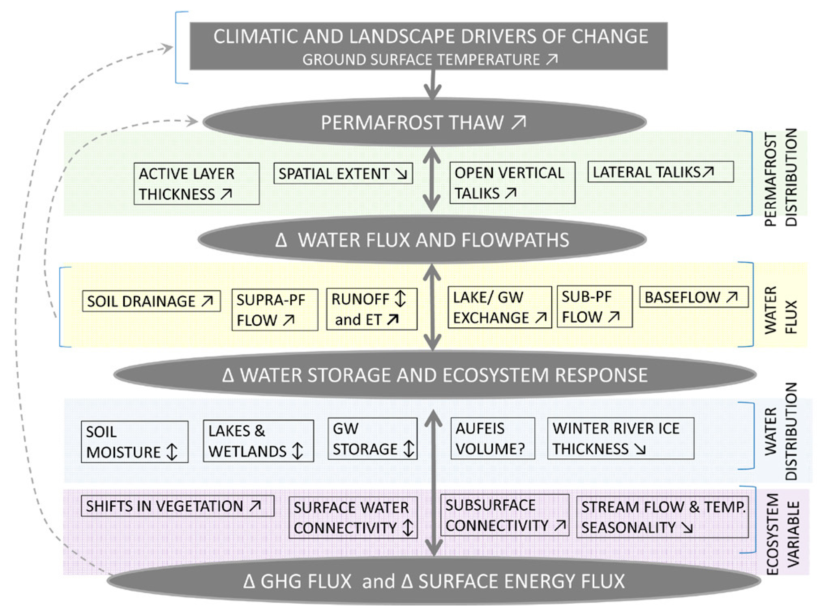
1.3. The Impacts of Permafrost Thawing on the Arctic Hydrological Processes

Climate change is expected to alter the hydrological processes in the Arctic [6,18], e.g., through thawing of the permafrost layer, which has been observed from the field measurement data obtained during the last decades [19,20,21,22,23,24]. Global warming is expected to lead to permafrost degradation through changes in the three-dimensional distribution of permafrost (Figure 1), e.g., via changes in the active layer thickness (ALT) [8,25,26,27,28], spatial extent [26], open vertical taliks [29], and lateral taliks [30]. The thawing of permafrost is expected to change both surface and subsurface hydrology in the Arctic [31]. Permafrost thawing leads to alterations in: (1) Water fluxes and flow paths, including increasing soil drainage, increasing suprapermafrost flow (SUPRA-PF) [32], runoff variation [33], increasing evapotranspiration (ET), increasing the exchange of water flow between lakes and groundwater [34], increasing subpermafrost flow (SUB-PF), and increasing baseflow [35,36,37,38]; (2) secondly, water storage and ecosystem responses including water distribution, e.g., variation in soil moisture [39], lakes and wetlands [40,41], groundwater (GW) storage [42,43]), aufeis (icing) volume [44], decreasing winter river ice thickness [45], and ecosystem variables, e.g., increasing vegetation [46,47], variation in surface water connectivity [48], increasing subsurface connectivity, decreasing streamflow, and temperature seasonality [49]; and (3) also alterations in greenhouse gasses (GHGs) and the surface energy flux [50]. It is projected that, because of permafrost degradation under global climate change, surface water systems will be transferred to more groundwater-based systems in large-scale assessments of the Arctic region [31].

1.4. Importance of Choosing the Suitable Modeling Tools for the Arctic Region

It has been demonstrated that the presence of permafrost has a high impact on hydrological processes in the Arctic. The changes of Arctic hydrology (including surface and subsurface hydrology) are expected to be more complicated under the context of global climate change, which causes permafrost degradation and changes in other related processes. Hydrological models are state-of-the-art tools for the investigation of global climate change impacts, and numerous models have been developed in recent decades. Both surface and subsurface hydrological models have demonstrated their capacities to simulate permafrost hydrology. For example, many surface hydrological models have approached analytical solutions (by using a simple heat transfer equation, e.g., Stefan’s equation) and numerical solutions (e.g., finite difference, finite element, and finite volume methods) to simulate the seasonal freezing–thawing process. Many subsurface hydrological models have coupled a three-dimensional (3D) equation for water flow (e.g., the 3D Richards equation) and a three-dimensional equation for heat transfer, especially considering the three phase changes of water in near-surface soil. However, both surface and subsurface hydrological models still have their limitations when dealing with permafrost hydrology. For example, one-dimensional (vertical direction) heat transfer, used in surface hydrological models, cannot be used to simulate multidecadal and multidimensional changes. Additionally, surface hydrological models still lack important processes in permafrost environments, such as consideration of heat capacity, thermodynamic equilibrium, and the three phase changes (ice, liquid, and gas) of water in near-surface soils. Subsurface hydrological models do not feature land surface schemes in their structures and have complex boundary conditions, and they are also difficult for non-expert users to use, etc. Moreover, sparse data of the Arctic make it more difficult to collect the necessary input data for the models. Therefore, finding suitable models for the Arctic is a challenge for hydrological modelers. The current paper presents a review and analysis of the functions, advantages, and disadvantages of different hydrological models and evaluates their suitability for simulating hydrological processes in the Arctic region. The selection of suitable models is carried out via answering the following pertinent questions:
1.
Do the models consider the important processes in permafrost environments, including the following factors:
  • Surface energy balance;
  • Snow processes, snow insulation, and snow melt;
  • Infiltration processes;
  • The dynamics of soil thermal and soil moisture fluxes;
  • Soil heterogeneities;
  • The dynamics (seasonal thawing) of the active layer;
  • Subsidence;
  • A three-phase change of water (ice, liquid, and gas) during the freezing and thawing of near-surface soil.
2.
Can the models be widely applied for Arctic permafrost, particularly considering the following requirements:
  • Requirement for input data, i.e., large or small requirement;
  • Requirement for computation processes, i.e., strong or low requirement;
  • Ability to be applied with different sizes of watersheds, i.e., small-scale and/or large-scale.

2. Some Well-Known Hydrological Models Applied in the Arctic

2.1. Topoflow Model

Topoflow is a spatially distributed and process-based hydrological model that was firstly designed for Arctic and sub-Arctic basins [6]. Topoflow has the capacity to simulate hydrological processes in permafrost environments, including the surface energy balance, snowmelt (using simple degree day or full energy balance methods), infiltration (using Green–Ampt, Smith–Parlange, or 1D Richards’ equation with three layers), and volumetric soil moisture content (using Darcian theory with multiple uniform layers). Moreover, Topoflow is able to reasonably simulate the ALT with a relatively simple method. However, such a method should be further improved in order to analyze the dynamics of the active layer more accurately, since the active layer has a high impact on the hydrological processes in permafrost environments [51]. The simulation of subsidence and a three-phase change of water (ice, liquid, and gas) during the freezing–thawing process of the near-surface soil is not mentioned in the Topoflow model.
The Topoflow model was applied in a small-scale watershed in the Arctic, Imnavait Creek, (around 2 km2) in Alaska, United States, which was underlain by continuous permafrost [6]. The results showed that the model has good performance for simulation of the hydrological cycle, including evapotranspiration, snowmelt, infiltration, runoff, and energy balances in the Arctic [6]. The hydrology change of the Imnavait Creek watershed under different climate change scenarios was also simulated [6], including evaluation of the performance of the model. The model has some limitations, such as the spatial variability of the active layer’s depth (not presented in the model) and the simplification of the complex soil moisture heterogeneity, etc.

2.2. DMHS Model

The DMHS (deterministic modeling hydrological system) model was developed for both mountainous and flat topographies, including basins with different climate zones, regardless of their scales [52]. This model can be applied to any geographical area in the world [53]. The DMHS model is a kind of physically-based, semi-distributed model for runoff estimation. The model can simulate the important processes in permafrost-affected regions, such as the surface energy balance, snow accumulation, snowmelt, sublimation, infiltration, soil heterogeneity, heat and water dynamics, and phase changes in soil layers [52,53,54,55,56]. Additionally, DMHS can also simulate the dynamics of the ALT with reliable results [57].
Vinogradov et al. [52] applied the DMHS model to six mountainous watersheds of different sizes, with areas varying from 40 to 2.4 million km2 across eastern Siberia and inside the Lena River basin in the Arctic region, showing promising results. However, the DMHS model has limitations regarding the routing scheme, which is especially not applicable to rivers which have a backwater phenomenon [58]. Another limitation of the DMHS model is the difficulty in the acquisition of soil profile properties in a required format for the model [52]. This could be a limiting factor for its wide application in the Arctic, where the available data are usually limited.

2.3. HBV Model

The HBV (Hydrologiska Byråns Vattenbalansavdelning) model is a rainfall–runoff model that was first successfully applied in 1972 [59,60,61,62,63]. The HBV model has developed significantly since then, and nowadays it is considered to be a standard tool for an increasing number of applications, such as flood forecasting, forecasts of inflow to reservoirs of hydropower dams, assessment of the impacts of climate change on water resources, or for the simulation of hazards in designing high hydropower dams, etc. [64,65,66,67]. The HBV model can be used as a semi-distributed, conceptual model. The HBV model considers the important processes of permafrost hydrology, such as the surface energy balance, snow routine, snow melt, soil moisture, and infiltration. Especially, the model uses an accumulated degree day coefficient, which is set up based on field measurement, to simulate the ALT [68]. In some case, the HBV model is coupled with other thermal hydrological models, e.g., the CryoGrid model, for simulation of the active layer dynamics [67].
The HBV model has been applied in more than 40 countries with different climate conditions [69]. In Nordic countries, the HBV model is currently used for flood forecasting and several other purposes, such as the simulation of design flood for supporting the design for spillway structures [70], water resource evaluation [71,72], and nutrient load estimates [73]. In Norway, the HBV model has been applied since 1983 [74] and has recently been considered as an important tool for water management by NVE (the Norwegian Water Resources and Energy Directorate). The model has been used for flood forecasting under the impacts of climate change [75].
The advantage of the HBV model is that it requires less input data and computer facilities, which is suitable for the sparse data in the Arctic region. Especially, the model could be a potential tool for hydrological simulation in ungauged river basins. However, obtaining the optimum model parameters for the HBV is not an easy task [64]. In addition, HBV model simplifies the equation for water storage in the catchment. Moreover, the HBV model requires the most basic input data, i.e., only daily precipitation and average daily air temperature, and these data are spatially averaged over the watersheds by Thiessen polygons. However, the Thiessen polygon method does not consider the elevation and temperature gradients in the basin. Hence, the interpolation method used in the HBV model could result in unsatisfactory modeling results.

2.4. SWAT Model

The SWAT (soil and water assessment tool) model [76] is a robust watershed modeling tool which was designed by the USDA (United States Department of Agriculture) Agricultural Research Service, the USDA Natural Resources Conservation Service, and the Texas A&M University. The model is currently used in more than 100 countries around the world. The SWAT is a physically-based, semi-distributed, watershed-scale model which operates on a daily time step [77,78]. The model was developed to simulate the impacts of land use management activities on water resources, sediment, and agricultural chemical yields [79] in large, complex, and ungauged watersheds with variation in soils, land uses, and management conditions over long periods of time [80,81]. Moreover, the model supports the understanding of complex ecosystems, climate change, and agricultural production issues around the world [82,83,84,85,86,87,88,89,90]. The SWAT model is capable of modeling river basins for thousands of square miles. Especially, it is able to simulate watersheds without requiring monitoring data. Regarding permafrost hydrology, the SWAT is able to simulate the surface energy balance, snow cover, snow melt, infiltration, soil moisture, soil heterogeneity, and lateral subsurface flow from the soil profile. Additionally, the SWAT takes into account the presence and development of the ALT in the model’s structure but only via using the average values [91]. Therefore, further development in the model’s structure to obtain a higher resolution for the spatiotemporal variation of the ALT is recommended, or otherwise coupling SWAT with other models to return better modeling results for the active layer dynamics. Moreover, simulation of soil heat transfer, snow insulation effects, and subsidence has not been developed yet for the SWAT model.
The SWAT model has been applied in many river basins in Europe and some regions in the Arctic. For instance, the SWAT model was applied to assess the variation of the hydrological regime and water quality under the impacts of human activities and climate change for the whole European territory [92]. In another study, the SWAT model was coupled with carbon modules to assess organic carbon exportation in an Arctic watershed via examination of the Yenisei River [91]. The advantage of the SWAT model is its capacity to model the temporal and spatial variations of hydrological process in large-scale Arctic watersheds [91]. The NRCS (Natural Resources Conservation Service) runoff curve number method in the SWAT provides a relatively easy way for the model to be adapted to a wide range of hydrological conditions [79].

2.5. WaSiM

The WaSiM (water balance simulation model) is a deterministic, spatially distributed hydrological model that was firstly developed during 1994-1996 by Jörg Schulla [93]. The model was designed to simulate water cycles in both surface and subsurface areas in river basins with variations in the spatial and temporal scales [93]. The WaSiM is able to simulate the hydrological processes for the catchments with sizes varying from <1 up to >100,000 km2 [93]. The WaSiM is able to solve several issues in river basins, including assessing the impacts of climate change and land use change on water resources, runoff forecasting, groundwater recharge, soil water, substance transport, etc. [93]. The model runs with time steps from minutes to several days [93]. The WaSiM can be used for both short-term (e.g., floods) and long-term (e.g., water balance) simulations [93]. The WaSiM is able to simulate the important hydrological processes in Arctic permafrost, including snow accumulation, snow melt, infiltration, soil moisture, and soil heterogeneities. Additionally, the model can simulate the ALT dynamics in permafrost regions. However, such simulation is relatively simple and is only based on empirical approaches. Particularly, the WaSiM calculates the thaw depth based on the simple formula given as follows [94]:
d thaw = α   n sf ,
where:
  • d thaw is the thaw depth (m);
  • α is an empirical coefficient (~0.02, …, 0.05);
  • n sf is the number of snow-free days.
Since the calculation approach in Equation (1) is relatively simple, in order to simulate the freezing–thawing process of the active layer more accurately, a physically-based heat transfer model is recommended [94].
The model is able to deal with soil heat flux. It provides the variations of soil temperatures in three dimensions. In addition, the WaSiM considers phase changes, which allows the model to simulate the freezing and thawing of an active layer in permafrost environments [95]. However, the drawbacks of the WaSiM is its high sensitivity to temporal and spatial resolutions. Therefore, the model is not suitable for transfer to other scales without recalibration. Moreover, the WaSiM requires intensive input data and model parameters for each grid cell of the model domain since it is a fully distributed model. This is considered as a big challenge in light of the scarce data in the Arctic region.
The WaSiM was first applied in the Arctic watershed by Liljedahl [93]. The long-term water balance during 1999–2009 was evaluated and its changes under global climate change in the permafrost-dominated watersheds were projected, such as the two vegetated drained thaw lake basins near Utqiaġvik, formerly known as Barrow, in the north of Alaska. In another study, WaSiM was applied to assess the influence of permafrost degradation on the Arctic tundra hydrology [96].

2.6. ECOMAG Model

The ECOMAG (ecological model for applied geophysics) model is a physically-based, distributed hydrological model for the simulation of hydrological cycles and water quality transformation in catchments in cold climate regions [97,98]. The model includes two separate submodels, e.g., a hydrological submodel and a water quality submodel, which operate at a daily time step. The hydrological submodel describes several processes occurring in the catchments, including surface runoff, evapotranspiration, infiltration into soil layers, soil moisture, and subsurface flow. It is able to simulate the hydrothermal processes, which are important in permafrost regions, including the formation of snow cover, snowmelt rate (using the degree day method), ALT dynamics, infiltration of snowmelt into the unfrozen and frozen soils by integrating the governing equations of basic hydrodynamic and thermodynamic of water, heat vertical transfer, horizontal water flow, etc. [99]. The water quality submodel simulates the pollution transformation process from point sources and non-point sources in the catchment, including geochemical processes and the biochemical degradation process of dissolved organic pollutants.
The ECOMAG model was tested for hydrological simulation in numerous river basins in cold climate regions such as Canada, Russia, Norway, and Sweden. The model has been applied in the large Arctic basins, including the Mackenzie River basin in Canada, with satisfactory performance [100], and the Lena River basin in Russia, also with satisfactory performance [101]. Additionally, the ECOMAG was approached to investigate climate change impacts on the water regimes of those river basins [102,103].

2.7. CRHM Model

The CRHM (cold regions hydrological model) is a physically-based, semi-distributed model developed for hydrological cycle simulation over small to medium river basins in cold climate regions [104]. The CRHM is a flexible, object-oriented modeling system with the capacity to simulate a wide range of important permafrost-related processes in the cold regions, including snow processes (e.g., snow redistribution by wind, snow interception, sublimation, snowmelt, and infiltration of snowmelt into unfrozen and frozen soils), glacier melts, actual evaporation and evapotranspiration, radiation exchange, and soil moisture balance, etc. The CRHM is able to simulate the ALT dynamics by approaching Stefan’s heat flow equation [105] as follows:
ξ = 2 kF Lw ρ ,
where:
  • ξ is the frost/thaw front depth (m);
  • k is the thermal conductivity of the soil (W m−1 k−1);
  • F is the surface freeze/thaw index (°C degree days);
  • L is the latent heat of fusion (J kg−1);
  • w is volumetric water content (m3 m−3);
  • ρ is the bulk density of the soil (kg m−3).
The CRHM is flexible in terms of its spatial solutions (from lumped to distributed) and model structures (from conceptual to physically-based), depending on the objectives of the studies and available input data for catchments. This is considered as a benefit for use in the Arctic region, which features sparse data. However, there is no required calibration for the model, and the model parameters are normally obtained based on the expert knowledge of the modeled catchment. Therefore, the modeling results have high uncertainty.

2.8. ATS Model

The ATS (arctic terrestrial simulator) model, which was developed from Amanzi code [106], is an integrated tool of the permafrost-related process model and the physically-based model [107]. The model couples the surface energy balance model [108] and the three-dimensional (3D) subsurface thermal hydrology model [109,110] for multidimensional simulations in permafrost-affected regions. The model employs the diffusion wave equation to simulate the surface hydrology, energy transport, and phase change. However, simulation of the dynamic topography due to the influence of thaw-induced subsidence has not been developed yet.
The ATS model is an open source model and one of the first tools for addressing fully-coupled surface/subsurface permafrost thermal hydrology in multidimensional simulations, which is considered as the existing challenge for hydrological models in permafrost environments. By approaching a novel multiphysics management system [111] to increase the complexity of the model, the ATS model can meet the challenge of operating many numerical models in permafrost regions, i.e., performing nonlinear constitutive modeling, phase change modeling, the coupling of several processes in different spatial domains, the ability for simulating transitions among different states on the land surface, and the possibility for using an unstructured grid according to the given topographical features. Moreover, the ATS model has a fine-scale structure and is suitable for the specific topography of the polygonal Arctic tundra, which requires a high spatial resolution, large spatial model domain, and large grid size because of long-range surface flow. Therefore, the incorporation of the extension ATS code with good parallel scaling of the Amanzi code becomes a potential tool for investigating the responses of small-scale topographic features in permafrost environments in the context of global climate change. Moreover, the ATS is able to simulate comprehensive snow processes, such as an increasing snow density with snow age, snow insulation, and snow thermal conduction [107].
However, the ATS model has limitations regarding (1) solving the convergence of nonlinear systems around the transition between freezing and thawing [112] and (2) simulating topography change by subsurface ice melting requiring the movement of grid/mesh cells but having to maintain the water and energy balance inside the moving grid cells.

2.9. CryoGrid 3 Model

The CryoGrid 3 model is a new, simple, and one-dimensional land surface model developed to simulate ground surface temperatures in permafrost-affected regions. The model was built based on the thermal permafrost model CryoGrid 2 [113] by developing further calculation of the surface energy balance and modifying the snow scheme, which are important factors in permafrost hydrology processes. The CryoGrid 3 model is considered as the upper boundary condition of the CryoGrid 2 model. The surface energy balance describes the processes of energy transfer between the atmosphere and the ground. Such processes include the radiation balance, the exchange of sensible heat, evaporation, etc. [114], as described in the following equation:
E t = S in + S out + L in + L out + Q h + Q e + Q g ,
where:
  • S in , S out are the short-wave radiation input and output, respectively (W m−2);
  • L in , L out are the long-wave radiation input and output, respectively (W m−2);
  • Q h , Q e , Q g are the sensible, latent, and ground heat fluxes, respectively (W m−2).
The CryoGrid 3 model is able to simulate other important processes in permafrost-affected regions, including subsurface heat transfer (considering the phase change of soil water), energy transfer, and mass balance of the snowpack. The subsurface thermal scheme is described by the concept of conductive heat transfer via Fourier’s law as the following equation:
c eff ( z , T ) T t z ( k ( z , T ) T z ) = 0 ,
where:
  • c eff ( z , T ) is the effective volume capacity (J m−3 K−1);
  • k ( z , T ) is the thermal conductivity (W m−1 K−1).
The energy transfer within the snowpack is conductive heat transfer, which is similar to the soil, as in the following equation:
c snow ( z , T ) T * t z ( k snow ( z , T ) T * t ) = 0 ,
where:
  • c snow ( z , T ) is the snow heat capacity (J m−3 K−1);
  • k snow ( z , T ) is the thermal conductivity of the snow (W m−1 K−1);
  • T * is the snow temperature (°C).
The CryoGrid 3 model is run in the MATLAB programming environment. The model has simple code and is open for modification. Therefore, the CryoGrid 3 model can be considered as a platform to integrate further processes in permafrost environments.
The CryoGrid 3 model has been tested in Arctic conditions with the large Lena River basin and showed satisfactory results to simulate the surface temperature, surface energy balance, ground temperature, ALT, and ground subsidence [115]. However, it is not guaranteed that the model could perform well in other permafrost basins. Instead, further considerations should be made before applying the model to a wider range of permafrost-affected regions. The CryoGrid 3 model has three major challenges [115]: (1) The model considers relatively simple snow processes (e.g., the assumption of a constant density of snowfall); (2) secondly, it is unclear that the model could perform well with the simulation of energy transfer and ground thermal regimes in regions with high vegetation cover; and, finally, (3) the simulation of the water balance needs further improvements, particularly for the simulation of seasonal changes.

2.10. GEOtop Model

The GEOtop model is a physically-based, distributed hydrological model that couples the water and energy balance [116,117]. The model was developed specifically for small catchments and complex mountain terrains. The GEOtop model combines the strengths of both land surface models and flood forecasting models [117]. In the GEOtop model, the interaction of topography with radiation is treated in detail, which is normally not considered in many hydrological models. The model simulates not only the energy balance (e.g., evapotranspiration and heat transfer) but also the water cycle (e.g., cycles of water, snow, and glaciers). The energy and mass balance is calculated based on a 3D Richards equation [118] and a 1D energy equation [112]. Vegetation, which contributes to the turbulent fluxes, is calculated based on a double layer scheme [119]. The snow processes (e.g., snow accumulation and snowmelt) are simulated by a multilayer discretization of the snowpack [120]. Additionally, a blowing snow module [121,122] is also included in the model to calculate the accumulation and blowing of snow because of wind.
The GEOtop model has been applied in a wide range of studies, including studies of soil water content [123], evaporation from soil [124,125], transpiration from vegetation [119], snow in basins [120,126,127], surface temperature [125], the temperature of soil and rock under freezing conditions [128], the mass balance of glaciers [129], interactions between the ground water table and thaw depth [118], and discharge at basin outlets [116].
The GEOtop model is a fully distributed model and requires intensive inputs, model parameters, field measurements, and experiments, as well as intensive computation. Additionally, modification of the code in the GEOtop model is not allowed, unlike other cryo-hydrogeological models (e.g., CryoGrid 3 or SUTRA-ICE).

2.11. SUTRA-ICE Model

The SUTRA-ICE [130] model was developed by modification of the existing SUTRA (saturated/unsaturated transport) numerical model [131,132] in order to simulate the processes of subsurface ice formation and melting, which is important for heat transport, groundwater, and biological activities in permafrost environments [130]. Basically, the SUTRA model is a finite element numerical model for the simulation of saturated/unsaturated groundwater flow and solute energy transport. Regarding the working mechanisms, the SUTRA model approaches the problem via a two-dimensional hybrid method (e.g., finite element and finite difference methods) to describe two interdependent processes, including: (1) Fluid density-dependent saturated or unsaturated groundwater flow; and (2) the transport of a solute or thermal energy in groundwater flow, as well as in the solid matrix of the aquifer. Especially, the SUTRA model has the capacity to model the thermal regimes, thermal energy storage, and thermal pollution in aquifers, and additionally subsurface heat conductivity, geothermal reservoirs, and natural hydrogeological convection. In addition, the SUTRA model has been applied to investigate the impacts of climate change on permafrost thawing, ALT dynamics, and groundwater flow in cold climate regions [133,134,135,136,137,138]. Besides the functions existing in the SUTRA version, the modified SUTRA-ICE (with 2-dimensional and 3-dimensional versions) model can deal with the subsurface, saturated/unsaturated freezing processes (including phase changes), latent heat, permeability, heat capacity, thermal conductivity, and liquid porosity [139]. The SUTRA-ICE model has demonstrated its high capacity to simulate the formation and melting of near-surface ice and subsurface temperature distribution in cold climate region in previous studies [140]. The SUTRA-ICE model is a free model (applying for version 3.0) and it allows users to modify the code for further development. This is considered as an advantage of the model. However, the model has some challenges [139]: (1) The boundary conditions are complex; (2) it is still a problem to simulate freezing in unsaturated zones; (3) the model is not accurate for the simulation of active layer dynamics when the pore space is filled with both liquid and ice; (4) intensive computation is required; (5) the model is not able to utilize massive parallel computing hardware [109]; and (6) field verification is needed.

2.12. PFLOTRAN-ICE Model

The PFLOTRAN-ICE is a non-isothermal, single component (water), three-phase (ice, liquid, and gas) numerical model that has been recently developed to simulate subsurface hydrology in permafrost-affected regions [141]. The model calculates the balance of mass and energy for water components in three phases (ice, liquid, and gas) via the following equations [142]:
t [ ( s g η g X w g + s l η l + s i η i ) ] + . [ v l η l ] . [ s g τ g η g D g X w g ] = Q W ,
t [ ( s l η l U l + s g η g U g + s i η i U i ) + ( 1 ) ρ r c r T ] + . [ v l η l H l ] . [ k T ] = Q e ,
v l = k rl k μ l [ p l + ρ l gz ] ,
where:
  • Subscripts l, g, and i, are the liquid, gas, and ice phases, respectively;
  • ∅ is the porosity (-);
  • s l , s g , s i (constraint: s l + s g + s i = 1) are saturation indices of the liquid, gas, and ice phases, respectively (m3 m−3);
  • η l , η g , η i are the molar densities of the liquid, gas, and ice phases, respectively (kmol m−3);
  • X w g is the mole fraction of H2O in the gas phase (-);
  • τ g is tortuosity of the gas phase (-);
  • D g is the diffusion coefficient in the gas phase (-);
  • T is the temperature (it is assumed that all the phases and soil are in thermal equilibrium) (K);
  • c r is the heat capacity of the soil (J K−1);
  • ρ r is the density of the soil (kg m−3);
  • U l , U g , U i are the molar internal energies of the liquid, gas, and ice phases, respectively (kJ mol−1);
  • H l is the molar enthalpy of the liquid phase (kJ mol−1);
  • Q W is the mass source of H2O (kmol m−3 s−1);
  • Q e is the heat source (kmol m−3 s−1);
  • ( ) is the gradient operator (-);
  • .   ( ) is the divergence operator (-);
  • v l is Darcy velocity of the liquid phase (m s−1);
  • k rl is the relative permeability of the liquid phase (-);
  • k is the absolute permeability (m2);
  • ρ l is mass density of the liquid phase (kg m−3);
  • p l is the partial pressure of the liquid phase (Pa);
  • g is acceleration because of gravity (m s−2);
  • z is the vertical distance from a reference datum (m).
Together with the above balance equations, further requirements for the constitutive relationships (e.g., the mole fraction of water vapor, saturations of the phases, thermal conductivity, relative permeability, and water vapor diffusion coefficient) for the simulation of non-isothermal elements and the multiple phases of water are also described in the PFLOTRAN-ICE model.
The PFLOTRAN-ICE model makes use of the capacity in the PFLOTRAN code [143] for finding highly-scalable, parallel subsurface multiphysics solutions. Therefore, the model can simulate the degradation of ice wedge polygon bogs, which requires elucidation of three-phase change and relatively large model domains [144]. Although the PFLOTRAN-ICE model considers one component (water), the model is able to produce similar results to the more complicated two-component model [142] for the same application. This could be an advantage for the simulation of permafrost hydrology by using fewer demanding components (e.g., a single component of water substance). Moreover, the PFLOTRAN-ICE model is suitable for the large-scale range of model domains (i.e., kilometer scales).
However, the PFLOTRAN-ICE model does not consider surface flows, the surface energy balance, and topography dynamics because of permafrost thawing and the melting of ground ice. Such processes are expected to be coupled with subsurface hydrology for the comprehensive modeling of hydrology in permafrost-dominated regions [144].

2.13. The Present Capacities and Challenges of Hydrological Models to Deal with Permafrost Hydrology in the Arctic

2.13.1. Surface Hydrological Models

Surface hydrological models have demonstrated their capacity to simulate the seasonal freeze–thaw process in soil by approaching analytical and numerical solutions [25]. Regarding the analytical solutions, many physically-based models have incorporated a simple heat transfer equation (e.g., Stefan’s equation [145]) into their structure to deal with the soil freeze–thaw process. Because of the simplification of soil freeze–thaw algorithms, simulation for large-scale basins is an advantage [146,147]. Additionally, Stefan’s equation may be easily modified to include other processes, such as the temporal variation of soil moisture [148], spatial variation of the moisture content, thermal properties [149], the freezing–thawing process in two directions [150], heat advection [151], and the soil heat capacity [152]. Beside the analytical solutions, some surface hydrological models, especially distributed models [153,154,155,156], have approached numerical solutions (e.g., via finite difference, finite element, and finite volume methods) to simulate the ground freezing–thawing process. Such numerical approaches are able to deal with complex conditions (e.g., varying soil heterogeneities and complex temperature boundaries) or complex processes (e.g., coupling heat and water transfer, discontinuous freezing–thawing process, and the temporal variation of thermal factors). Compared to analytical solutions, numerical solutions perform better in the context of the freezing–thawing process in the ground [147]. For example, numerical solutions simulate the freezing and thawing process in soil over a wide range of temperatures, unlike the assumption of sharp change by analytical solutions. Therefore, such a freezing range permits some subsurface water flow at sub-zero temperatures.
However, there are still numerous challenges for surface hydrological models in permafrost environments [25]. First of all, many surface hydrological models coupled with numerical soil freezing models only consider a vertical direction of heat transfer but ignore the lateral direction, which is crucial to the isolated and discontinuous permafrost bodies located in the lowland regions [157,158], as well as in steep and alpine regions [159,160]. Therefore, one-dimensional heat transfer is only suitable for simulating the seasonal freeze–thaw process of permafrost, but not for multidecadal and multidimensional changes. Secondly, many surface hydrological models do not consider the important factors influencing the rate of the freezing–thawing process in soil, such as the heat capacity and soil layering. A lack of those factors could result in an inaccurate calculation of frost, depths of thawing, subsurface water storage, and groundwater routing. Thirdly, many surface hydrological models or numerical models of soil freezing–thawing processes do not represent the thermo-dynamic equilibrium well, particularly the disequilibrium phase change processes occurring during freezing and thawing, as well as disequilibrium pressure during the infiltration of snowmelt into partially frozen soils. Fourthly, surface hydrological models, even complex physically-based models, cannot accurately simulate the ground surface temperature, which controls the seasonal freezing–thawing process of soil under snowpack and snow-free conditions. This is because ground thermal regimes can be highly sensitive to model parameters [140,161,162]. Lastly, in permafrost environments, surface hydrological models are still unable to clearly represent the relationship between the hydraulic conductivity (K) of soil and the ice, liquid, and gas existing in partially frozen and unsaturated soils. For example, it is unclear whether the K factor of partially frozen soils is decreased or not by resistance factors.

2.13.2. Subsurface Hydrological Models/Groundwater Models/Cryo-Hydrogeological Models

Several one-dimensional groundwater models, coupled with energy transport models, have been developed to simulate the freezing and thawing process in soil since the 1970s. However, the simulation is only limited to the vertical direction. In the last decade, many multi-dimensional models have been developed to support groundwater simulation in permafrost environments [109,130,141,163,164]. Such models work by coupling a three-dimensional equation for water flow (the Richards equation) into a three-dimensional equation for heat transfer (e.g., heat conduction, heat advection, and thermal dispersion). Such models are also known as cryo-hydrogeological models, and they take into account the pore water phase change [165] and the impacts of the latent heat of it on the effectiveness of subsurface heat capacity, as well the decreasing hydraulic conductivity of soil because of the formed pore ice. Moreover, cryo-hydrogeological models have been approached in numerous studies of climate change impacts (e.g., the increase of the ALT) on groundwater (e.g., increase of baseflow and the groundwater exchange between supra-permafrost and sub-permafrost aquifers) in permafrost basins [134,135,136,137,138,157,166,167,168,169,170].
Beside the existing achievements, the cryo-hydrogeological models have several limitations. First of all, most of the models have been applied in ideal environmental conditions, except for a few studies conducting investigations under field conditions [108,157,171]. This is due to the lack of hydrogeological data at high altitude or latitude regions. Secondly, most of the cryo-hydrogeological models do not include the land surface scheme and thermal processes in their structure. Therefore, the boundary conditions for such models must be subsurface conditions, such as the groundwater table, groundwater recharge rate, and soil temperature. However, such input data are limited and they are normally simplified and assumed. Thirdly, the models are limited into two dimensions with simplified structures, only considering small-scale areas. Additionally, the models require a fine grid structure and a small time step for application. Therefore, intensive computational processes are normally expected for the high spatial and temporal resolutions required. Finally, most of cryo-hydrogeological models are difficult for non-expert users to use because of their complexities.

2.14. Model Comparison Regarding the Capacities of the Models to Deal with Permafrost Hydrology in the Arctic

This section aims to summarize and identify the capabilities of the twelve well-known hydrological models for simulating Arctic permafrost hydrology. Permafrost is an important feature affecting hydrological processes in the Arctic. The main factor dominating water storage and transmission in permafrost basins is the ground thermal regime, which has been identified as the typical challenge of hydrological models in permafrost environments [31]. In addition to the ground thermal regime, other important processes related to permafrost hydrology and the Arctic conditions should be considered, such as the surface energy balance, snow process, snow insulation (influencing the air–soil temperature relationships), snowmelt, infiltration, soil heterogeneities, soil moisture regime, the three-phase change of water (ice, liquid, and gas) during the freezing–thawing process of near-surface soil, as well as the dynamics of the ALT. Therefore, the most suitable models for application in permafrost conditions should include as many of the important processes as possible. Table 1 summarizes the important processes for permafrost hydrology that are considered in each model’s structure.
According to Table 1, the important processes in permafrost environments considered in the model include: (1) Surface energy balance; (2) snow process; (3) snow insulation; (4) snowmelt; (5) infiltration; (6) soil thermal; (7) soil moisture; (8) soil heterogeneities; (9) active layer thickness (ALT) dynamics; (10) subsidence; and (11) three-phase change of water during the freezing–thawing process in near-surface soils. Additionally, the symbol of √ denotes available and the abbreviation of n/a defines not available, unclear, or no information.
The twelve hydrological models may be classified into two major groups. The first group are surface hydrological models, including Topoflow, DMHS, HBV, SWAT, WaSiM, ECOMAG, and CRHM. The second group are cryo-hydrogeological models, including ATS, CryoGrid 3, GEOtop, SUTRA-ICE, and PFLOTRAN-ICE. Generally, each model group has its own competences and limitations in dealing with permafrost hydrology, as addressed in prior sections. The first model group performs well for the simulation of surface hydrology, but the capacities of these models to simulate sophisticated ground thermal processes, groundwater flow, or other processes related to permafrost degradation are low. For instance, most of models in group 1 are not able to take into account the influences of snow insulation on air–soil temperature relationships, as well as a required three-phase change of water in permafrost soil (except for DMHS and WaSiM). Some models exclude the important soil thermal process in their structure, such as Topoflow, HBV, and SWAT. None of the surface hydrological models are able to simulate the subsidence as a result of permafrost thawing. On the contrary, many cryo-hydrogeological models are able to simulate subsurface hydrological processes well.
Most of the cryo-hydrogeological models consider a required three-phase change in permafrost environments. Exceptionally, the SUTRA-ICE and PFLOTRAN-ICE models do not include land surface schemes and only simulate the subsurface hydrology. These two models are also not able to simulate the subsidence. Interestingly, almost all of the twelve models in the two groups have capacities to simulate the dynamics of the ALT. However, the accuracy or reliability of the simulation results are not the same for each model. Topoflow, HBV, SWAT, WaSiM, and SUTRA-ICE have low model performance, since they approach a relatively simple method for the simulation of the active layer dynamics, and they lack consideration of spatiotemporal variation.

2.15. Model(s) Selection for the Arctic

Concerning the specific hydrological processes and the sparse data of the Arctic region, the selection of a suitable model should fulfil two main criteria: (1) The capability of the model to deal with unique permafrost hydrological processes; and (2) the possibility to be applied with moderate amounts of data. Table 2, Table 3, Table 4 and Table 5 summarize the main criteria as a basis to choose suitable models for application in the Arctic region. Since the freezing and thawing process of the ALT strongly impacts hydrological processes in the Arctic, the ALT was prioritized among other factors listed in Table 1 for selection of the suitable models for the Arctic.
First of all, if a study aims to only evaluate the surface hydrology process, Topoflow, HBV, SWAT, ECOMAG, and CRHM could be solutions, since they have been verified in many different case studies. Particularly, the conceptual model HBV and the physically-based, semi-distributed SWAT and CRHM models fit best for catchments with moderate data requirements, while the physically-based, distributed models Topoflow and ECOMAG require intensive inputs for every cell of the catchment.
Secondly, if the accuracy of subsurface hydrology simulation is prioritized, DMHS, WaSiM, and the cryo-hydrogeology models are good options, since such models take into account the three phase changes of water, which are important in permafrost environments for analyzing water during the freezing and thawing process of near-surface soils. Other models also have capacities to simulate the subsurface hydrology, but their performances are lower. Further, some cryo-hydrogeology models, e.g., GEOtop, SUTRA-ICE, and PFLOTRAN-ICE, are only suitable for applications in small-scale study areas, while ATS and CryoGrid 3 can be applied to larger basins. Since SUTRA-ICE and PFLOTRAN-ICE do not include a land surface scheme in their structure, these models should be coupled with other land surface models for applications in the Arctic region.
Further, among the five cryo-hydrogeology models, the ATS model has demonstrated its capacity to comprehensively simulate snow processes. It takes into account the snow thermal conductivity, increasing snow density by snow age, and snow insulation. While other models, e.g., CryoGrid 3, have relatively simple snow simulation processes, the ATS and GEOtop models are the first tools that have coupled surface/subsurface permafrost thermal hydrology. Although, such models still have very few applications in the Arctic, so they should be widely tested.
Although the cryo-hydrogeology models appear to be potential tools for researching permafrost hydrology, they could be difficult for non-expert users because of their complicated model structures. Workshops or training should be helpful for new users. Moreover, it is normally difficult to collect enough input data for subsurface hydrological models in Arctic regions. Thus, coupling surface hydrological models as upper boundary conditions for subsurface hydrological models is recommended as one of the solutions, where the outputs from surface hydrological models would become inputs for the subsurface hydrological models. For example, outputs from the SWAT model, e.g., groundwater recharge, soil deep percolation, and stream stage, etc., could be used as inputs for groundwater models.
Thirdly, if the accuracy of ALT dynamics is targeted, DMHS, ATS, GEOtop, and PFLOTRAN-ICE are desirable choices. The other remaining models are not recommended for the study of ALT dynamics since their approaches are relatively simple, resulting in highly uncertainty for the simulation results.
Fourthly, choosing a proper model also depends on the available input data of the catchments and the study conditions (e.g., funding, etc.). Although the cryo-hydrogeology models have high capacities to simulate permafrost hydrology, they still present challenges in terms of gathering the required input data, especially for information about the subsurface boundary conditions in the Arctic. Therefore, it is very expensive to run such simulations.
Lastly, successful application of a model also depends on the knowledge and experience of the hydrologist users to the given model. For example, although HBV is a kind of conceptual, semi-distributed model, it has been widely used in Nordic regions, i.e., cold climate region. In addition, the ECOMAG and CRHM models are well-known in Russia and Canada, respectively (Figure 2). However, the application of CRHM requires accumulated knowledge and data of the study catchments, since there is no calibration procedure or testing cases for the model. This could present a challenge for non-expert or less experienced users.

3. Conclusions

The hydrological processes in the Arctic are more complicated than in other regions. Finding a suitable hydrological model to simulate and predict changes in the hydrological processes is therefore a challenging task for modelers. This paper has reviewed the functions, structures, operational mechanisms, and performances of twelve hydrological models that have previously been applied or have potential for application in the Arctic. Of them, the DMHS, ATS, GEOtop, and PFLOTRAN-ICE models are desirable options for the simulation of ALT dynamics, which has strong impacts on surface/subsurface hydrology. The three cryo-hydrogeology models GEOtop, SUTRA-ICE, and PFLOTRAN-ICE are only suitable for small-scale case studies, while the ATS and CryoGrid 3 models could be applied to large-scale catchments. The SUTRA-ICE and PFLOTRAN-ICE models appear to be suitable subsurface hydrological models. However, since they lack land surface schemes in their structures, they should be applied in tandem with other land surface models for the comprehensive simulation of permafrost hydrology. A significant revolution of hydrological modeling is the recently developed ATS and GEOtop models, which are the first tools that couple surface/subsurface permafrost thermal hydrology. It would be valuable to test the new models and to verify their performances in the Arctic condition. In the situation of only studying the surface hydrology, Topoflow, HBV, SWAT, ECOMAG, and CRHM could be good choices. Particularly, the semi-distributed models HBV, SWAT, and CRHM fit best for catchments with moderate data requirements, whereas the fully distributed models Topoflow and ECOMAG require intensive input data and model parameters. It is worth mentioning that since there is no required calibration procedure for the CRHM and Topoflow models, application of these models requires expert knowledge of the catchments, otherwise the modeling results could feature high uncertainty. Further, if the accuracy of simulating the subsurface hydrology in permafrost environments is targeted, DMHS, WaSiM, and the cryo-hydrogeological models are good options, since they consider the three phase changes of water during the freezing and thawing of near-surface soils. Finally, the selection of the suitable models for Arctic permafrost regions should be based on several factors, besides simulating the permafrost hydrology. Other factors, such as data acquisition, the required research period, and funding could influence the model selection and reliability of the results.

Author Contributions

M.T.B. initiated the idea, planned the scope, collected the information and data, structured and produced a draft manuscript, and performed revisions. J.L. supervised the progress, supported the idea, and conducted the review and editing. L.N. contributed to the reformulation of the paper structure, HBV hydrological model, language revision, and co-supervision of the review and revision processes. All authors have read and agreed to the published version of the manuscript.

Funding

This research received no external funding.

Acknowledgments

The authors would like to thank the Department of Technology and Safety, University of Tromsø—The Arctic University of Norway, for their financial support and administration for this study under project number 301184. Additionally, the publication charges for this article have been funded by a grant from the publication fund of UiT The Arctic University of Norway under project 551011. The collaboration with CSDI WaterTech is also highly appreciated. We especially thank the three anonymous reviewers for their constructive comments that helped to reasonably improve our manuscript. Finally, we also thank MDPI for English language editing, especially the English editor Max Kooij.

Conflicts of Interest

The authors declare no conflict of interest.

References

  1. Snow, Water, Ice and Permafrost in the Arctic (SWIPA): Climate Change and the Cryosphere; Arctic Monitoring and Assessment Programme (AMAP): Oslo, Norway, 2011.
  2. Snow, Water, Ice and Permafrost in the Arctic (SWIPA): Climate Change and the Cryosphere; Arctic Monitoring and Assessment Programme (AMAP): Oslo, Norway, 2017.
  3. Romanovsky, V.; Burgess, M.; Smith, S.; Yoshikawa, K.; Brown, J. Permafrost temperature records: Indicators of climate change. Eos 2002, 83, 589–594. [Google Scholar] [CrossRef]
  4. Woo, M.-K. Introduction. In Permafrost Hydrology; Springer Science and Business Media LLC: Berlin, Germany, 2012; pp. 1–34. [Google Scholar]
  5. Woo, M.-K. Active Layer Dynamics. In Permafrost Hydrology; Springer Science and Business Media LLC: Berlin, Germany, 2012; pp. 163–227. [Google Scholar]
  6. Schramm, I.; Boike, J.; Bolton, W.R.; Hinzman, L.D. Application of TopoFlow, a spatially distributed hydrological model, to the Imnavait Creek watershed, Alaska. J. Geophys. Res. Space Phys. 2007, 112, 1–14. [Google Scholar] [CrossRef] [Green Version]
  7. Walsh, J.E.; Anisimov, O.; Hagen, J.O.M.; Jakobsson, T.; Oerlemans, J.; Prowse, T.D.; Romanovsky, V.; Savelieva, N.; Serreze, M.; Shiklomanov, A.; et al. Cryosphere and hydrology, Chapter 6. In Arctic Climate Impact Assessment; Cambridge University Press: London, UK, 2005; pp. 184–242. [Google Scholar]
  8. Walvoord, M.A.; Voss, C.I.; Wellman, T.P. Influence of permafrost distribution on groundwater flow in the context of climate-driven permafrost thaw: Example from Yukon Flats Basin, Alaska, United States. Water Resour. Res. 2012, 48, 1–17. [Google Scholar] [CrossRef]
  9. Frampton, A.; Destouni, G. Impact of degrading permafrost on subsurface solute transport pathways and travel times. Water Resour. Res. 2015, 51, 7680–7701. [Google Scholar] [CrossRef]
  10. McNamara, J.P.; Kane, D.L.; Hinzman, L.D. An analysis of streamflow hydrology in the Kuparuk River Basin, Arctic Alaska: A nested watershed approach. J. Hydrol. 1998, 206, 39–57. [Google Scholar] [CrossRef]
  11. Hinzman, L.D.; Kane, D.L.; Benson, C.S.; Everett, K.R. Energy Balance and Hydrological Processes in an Arctic Watershed. In Ecological Studies; Springer Science and Business Media LLC: Berlin, Germany, 1996; Volume 120, pp. 131–154. [Google Scholar]
  12. Hinzman, L.D.; Bolton, R.W.; Petrone, K.; Jones, J.; Adams, P. Watershed hydrology and chemistry in the Alaskan boreal forest: The central role of permafrost. In Alaska’s Changing Boreal Forest; Chapin, F.S., III, Ed.; Oxford University Press: New York, NY, USA, 2006; pp. 269–284. [Google Scholar]
  13. Boike, J.; Roth, K.; Overduin, P.P. Thermal and hydrologic dynamics of the active layer at a continuous permafrost site (Taymyr Peninsula, Siberia). Water Resour. Res. 1998, 34, 355–363. [Google Scholar] [CrossRef]
  14. Bowling, L.C.; Kane, D.L.; Gieck, R.E.; Hinzman, L.D.; Lettenmaier, D.P. The role of surface storage in a low-gradient Arctic watershed. Water Resour. Res. 2003, 39, 1087. [Google Scholar] [CrossRef]
  15. Kane, D.L.; Hinzman, L.D.; Zarling, J. Thermal response of the active layer in a permafrost environment to climatic warming. Cold Reg. Sci. Technol. 1991, 19, 111–122. [Google Scholar] [CrossRef]
  16. Vörösmarty, C.J.; Hinzman, L.D.; Peterson, B.J.; Bromwich, D.H.; Hamilton, L.C.; Morison, J.; Romanovsky, V.E.; Sturm, M.; Webb, R.S. The Hydrologic Cycle and its Role in the Arctic and Global Environmental Change: A Rationale and Strategy for Synthesis Study; Arctic Research Consortium of the United States: Fairbanks, AL, USA, 2001; pp. 1–84. [Google Scholar]
  17. Slaughter, C.W.; Kane, D.L. Hydrologic role of shallow organic soils in cold climates. In Proceedings of the Canadian Hydrology Symposium 79: Cold Climate Hydrology, Vancouver, BC, Canada, 10–11 May 1979; pp. 380–389. [Google Scholar]
  18. Hinzman, L.D.; Bettez, N.D.; Bolton, W.R.; Chapin, F.S.; Dyurgerov, M.B.; Fastie, C.L.; Griffith, B.; Hollister, R.D.; Hope, A.; Huntington, H.P.; et al. Evidence and Implications of Recent Climate Change in Northern Alaska and Other Arctic Regions. Clim. Chang. 2005, 72, 251–298. [Google Scholar] [CrossRef]
  19. Lachenbruch, A.H.; Marshall, B.V. Changing Climate: Geothermal Evidence from Permafrost in the Alaskan Arctic. Science 1986, 234, 689–696. [Google Scholar] [CrossRef]
  20. Osterkamp, T. A thermal history of permafrost in Alaska. In Proceedings of the 8th International Conference on Permafrost, Zurich, Switzerland, 21–25 July 2003; pp. 863–868. [Google Scholar]
  21. Osterkamp, T.E. Characteristics of the recent warming of permafrost in Alaska. J. Geophys. Res. Space Phys. 2007, 112. [Google Scholar] [CrossRef]
  22. Wu, Q.; Zhang, T. Recent permafrost warming on the Qinghai-Tibetan Plateau. J. Geophys. Res. Space Phys. 2008, 113, 13108. [Google Scholar] [CrossRef]
  23. Batir, J.F.; Hornbach, M.J.; Blackwell, D.D. Ten years of measurements and modeling of soil temperature changes and their effects on permafrost in Northwestern Alaska. Glob. Planet. Chang. 2017, 148, 55–71. [Google Scholar] [CrossRef] [Green Version]
  24. Farquharson, L.M.; Romanovsky, V.E.; Cable, W.L.; Walker, D.A.; Kokelj, S.V.; Nicolsky, D. Climate Change Drives Widespread and Rapid Thermokarst Development in Very Cold Permafrost in the Canadian High Arctic. Geophys. Res. Lett. 2019, 46, 6681–6689. [Google Scholar] [CrossRef] [Green Version]
  25. Åkerman, H.J.; Johansson, M. Thawing permafrost and thicker active layers in sub-arctic Sweden. Permafr. Periglac. Process. 2008, 19, 279–292. [Google Scholar] [CrossRef]
  26. Mazhitova, G.G.; Malkova, G.; Chestnykh, O.; Zamolodchikov, D. Recent decade thaw depth dynamics in the European Russian Arctic based on the Circumpolar Active Layer Monitoring (CALM) data. In Proceedings of the 9th International Conference on Permafrost, Fairbanks, AL, USA, 29 June–3 July 2008; Institute of Northern Engineering, University of Alaska: Fairbanks, AL, USA, 2008; pp. 1155–1160. [Google Scholar]
  27. Brutsaert, W.; Hiyama, T. The determination of permafrost thawing trends from long-term streamflow measurements with an application in eastern Siberia. J. Geophys. Res. Space Phys. 2012, 117, 1–10. [Google Scholar] [CrossRef]
  28. Overeem, I.; Jafarov, E.; Wang, K.; Schaefer, K.; Stewart, S.; Clow, G.; Piper, M.; Elshorbany, Y. A Modeling Toolbox for Permafrost Landscapes. Eos 2018, 99, 1–11. [Google Scholar] [CrossRef]
  29. Smith, L.C.; Sheng, Y.; Macdonald, G.M.; Hinzman, L.D. Disappearing Arctic Lakes. Science 2005, 308, 1429. [Google Scholar] [CrossRef] [Green Version]
  30. Jepsen, S.M.; Voss, C.I.; Walvoord, M.A.; Minsley, B.J.; Rover, J. Linkages between lake shrinkage/expansion and sublacustrine permafrost distribution determined from remote sensing of interior Alaska, USA. Geophys. Res. Lett. 2013, 40, 882–887. [Google Scholar] [CrossRef]
  31. Walvoord, M.A.; Kurylyk, B.L. Hydrologic impacts of thawing permafrost—A review. J. Vadose Zone 2016, 15, 1–20. [Google Scholar] [CrossRef]
  32. Lyon, S.W.; Destouni, G. Changes in Catchment-Scale Recession Flow Properties in Response to Permafrost Thawing in the Yukon River Basin. Int. J. Clim. 2009, 30, 2138–2145. [Google Scholar] [CrossRef]
  33. Gelfan, A.N. Modelling hydrological consequences of climate change in the permafrost region and assessment of their uncertainty. In Proceedings of Cold Region Hydrology in a Changing Climate; Marsh, P., Ed.; IAHS: Wallingford, UK, 2011; Volume 346, pp. 92–97. [Google Scholar]
  34. Fedorov, A.; Gavriliev, P.P.; Konstantinov, P.Y.; Hiyama, T.; Iijima, Y.; Iwahana, G. Estimating the water balance of a thermokarst lake in the middle of the Lena River basin, eastern Siberia. Ecohydrology 2013, 7, 188–196. [Google Scholar] [CrossRef]
  35. Smith, L.C.; Pavelsky, T.M.; Macdonald, G.M.; Shiklomanov, A.I.; Lammers, R.B. Rising minimum daily flows in northern Eurasian rivers: A growing influence of groundwater in the high-latitude hydrologic cycle. J. Geophys. Res. Space Phys. 2007, 112, 1–18. [Google Scholar] [CrossRef] [Green Version]
  36. Walvoord, M.A.; Striegl, R.G. Increased groundwater to stream discharge from permafrost thawing in the Yukon River basin: Potential impacts on lateral export of carbon and nitrogen. Geophys. Res. Lett. 2007, 34, 1–6. [Google Scholar] [CrossRef] [Green Version]
  37. Jacques, J.-M.S.; Sauchyn, D.J. Increasing winter baseflow and mean annual streamflow from possible permafrost thawing in the Northwest Territories, Canada. Geophys. Res. Lett. 2009, 36, 1–6. [Google Scholar] [CrossRef]
  38. Rennermalm, A.K.; Wood, E.F.; Troy, T.J. Observed changes in pan-arctic cold-season minimum monthly river discharge. Clim. Dyn. 2010, 35, 923–939. [Google Scholar] [CrossRef]
  39. O’Donnell, J.A.; Jorgenson, M.T.; Harden, J.W.; McGuire, A.D.; Kanevskiy, M.Z.; Wickland, K.P. The Effects of Permafrost Thaw on Soil Hydrologic, Thermal, and Carbon Dynamics in an Alaskan Peatland. Ecosystems 2011, 15, 213–229. [Google Scholar] [CrossRef]
  40. Labrecque, S.; Lacelle, D.; Duguay, C.R.; Lauriol, B.; Hawkings, J. Contemporary (1951–2001) Evolution of Lakes in the Old Crow Basin, Northern Yukon, Canada: Remote Sensing, Numerical Modeling, and Stable Isotope Analysis. Arctic 2009, 62, 225–238. [Google Scholar] [CrossRef] [Green Version]
  41. Rover, J.; Ji, L.; Wylie, B.K.; Tieszen, L.L. Establishing water body areal extent trends in interior Alaska from multi-temporal Landsat data. Remote. Sens. Lett. 2011, 3, 595–604. [Google Scholar] [CrossRef]
  42. Muskett, R.R.; Romanovsky, V. Alaskan Permafrost Groundwater Storage Changes Derived from GRACE and Ground Measurements. Remote. Sens. 2011, 3, 378–397. [Google Scholar] [CrossRef] [Green Version]
  43. Velicogna, I.; Tong, J.; Zhang, T.; Kimball, J.S. Increasing subsurface water storage in discontinuous permafrost areas of the Lena River basin, Eurasia, detected from GRACE. Geophys. Res. Lett. 2012, 39, 1–5. [Google Scholar] [CrossRef] [Green Version]
  44. Yoshikawa, K.; Hinzman, L.D.; Kane, D.L. Spring and aufeis (icing) hydrology in Brooks Range, Alaska. J. Geophys. Res. Space Phys. 2007, 112, 1–14. [Google Scholar] [CrossRef] [Green Version]
  45. Beltaos, S.; Prowse, T. River-ice hydrology in a shrinking cryosphere. Hydrol. Process. 2009, 23, 122–144. [Google Scholar] [CrossRef]
  46. Chasmer, L.; Hopkinson, C.; Quinton, W. Quantifying errors in discontinuous permafrost plateau change from optical data, Northwest Territories, Canada: 1947–2008. Can. J. Remote. Sens. 2010, 36, S211–S223. [Google Scholar] [CrossRef]
  47. Baltzer, J.L.; Veness, T.; Chasmer, L.E.; Sniderhan, A.E.; Quinton, W.L. Forests on thawing permafrost: Fragmentation, edge effects, and net forest loss. Glob. Chang. Biol. 2014, 20, 824–834. [Google Scholar] [CrossRef]
  48. Connon, R.F.; Quinton, W.L.; Craig, J.; Hayashi, M. Changing hydrologic connectivity due to permafrost thaw in the lower Liard River valley, NWT, Canada. Hydrol. Process. 2014, 28, 4163–4178. [Google Scholar] [CrossRef]
  49. Liu, B.; Yang, D.; Ye, B.; Berezovskaya, S. Long-term open-water season stream temperature variations and changes over Lena River Basin in Siberia. Glob. Planet. Chang. 2005, 48, 96–111. [Google Scholar] [CrossRef] [Green Version]
  50. Lawrence, D.M.; Koven, C.D.; Swenson, S.C.; Riley, W.J.; Slater, A.G. Permafrost thaw and resulting soil moisture changes regulate projected high-latitude CO 2 and CH 4 emissions. Environ. Res. Lett. 2015, 10, 094011. [Google Scholar] [CrossRef] [Green Version]
  51. Bolton, W.R. Dynamic Modeling of the Hydrologic Processes in Areas of Discontinuous Permafrost. Ph.D. Thesis, University of Alaska Fairbanks, Fairbanks, AL, USA, August 2006. [Google Scholar]
  52. Vinogradov, Y.B.; Semenova, O.M.; Vinogradova, T.A. An approach to the scaling problem in hydrological modelling: The deterministic modelling hydrological system. Hydrol. Process. 2010, 25, 1055–1073. [Google Scholar] [CrossRef]
  53. Semenova, O.M.; Vinogradova, T.A. A universal approach to runoff processes modelling: Coping with hydrological predictions in data-scarce regions. In Proceedings of Symposium HS.2 at the Joint IAHS & IAH Convention; IAHS: Wallingford, UK, 2009; Volume 333, pp. 11–19. [Google Scholar]
  54. Vinogradov, Y.B. Mathematical Modelling of Runoff Formation. A Critical Analysis; Gidrometeoizdat: Leningrad, Russia, 1988. (In Russian) [Google Scholar]
  55. Semenova, O.; Lebedeva, L.; Vinogradov, Y. Simulation of subsurface heat and water dynamics, and runoff generation in mountainous permafrost conditions, in the Upper Kolyma River basin, Russia. Hydrogeol. J. 2013, 21, 107–119. [Google Scholar] [CrossRef]
  56. Semenova, O.; Vinogradov, Y.; Vinogradova, T.; Lebedeva, L.; Semenova, O. Simulation of Soil Profile Heat Dynamics and their Integration into Hydrologic Modelling in a Permafrost Zone. Permafr. Periglac. Process. 2014, 25, 257–269. [Google Scholar] [CrossRef]
  57. Lebedeva, L.; Semenova, O.; Vinogradova, T. Simulation of Active Layer Dynamics, Upper Kolyma, Russia, using the Hydrograph Hydrological Model. Permafr. Periglac. Process. 2014, 25, 270–280. [Google Scholar] [CrossRef]
  58. Finney, D.L.; Blyth, E.; Ellis, R. Improved modelling of Siberian river flow through the use of an alternative frozen soil hydrology scheme in a land surface model. Cryosphere 2012, 6, 859–870. [Google Scholar] [CrossRef] [Green Version]
  59. Bergström, S. Development and Application of a Conceptual Runoff Model for Scandinavian Catchments; Report RH07; SMHI: Norrköping, Sweden, 1976; pp. 1–134. [Google Scholar]
  60. Bergström, S. Parametervärden för HBV-Modellen i Sverige (Parameter Values for the HBV Model in Sweden); No 28; SMHI Hydrologi: Norrköping, Sweden, 1990; pp. 1–35. (In Swedish) [Google Scholar]
  61. Bergström, S. Principles and Confidence in Hydrological Modelling. Hydrol. Res. 1991, 22, 123–136. [Google Scholar] [CrossRef]
  62. Bergström, S.; Harlin, J.; Lindström, G. Spillway design floods in Sweden. I. New guidelines. Hydrol. Sci. J. 1992, 37, 505–519. [Google Scholar] [CrossRef] [Green Version]
  63. Bergström, S. Computer Models of Watershed Hydrology: The HBV Model; Singh, V.P., Ed.; Water Resources Publications: Highlands Ranch, CO, USA, 1995; pp. 443–476. [Google Scholar]
  64. Bergström, S. Experience from applications of the HBV hydrological model from the perspective of prediction in ungauged basins. IAHS Public 2006, 307, 97–107. [Google Scholar]
  65. Bøggild, C.E.; Knudby, C.J.; Knudsen, M.B.; Starzer, W. Snowmelt and runoff modelling of an Arctic hydrological basin in west Greenland. Hydrol. Process. 1999, 13, 1989–2002. [Google Scholar] [CrossRef]
  66. Wawrzyniak, T.; Osuch, M.; Nawrot, A.; Napiorkowski, J.J. Run-off modelling in an Arctic unglaciated catchment (Fuglebekken, Spitsbergen). Ann. Glaciol. 2017, 58, 36–46. [Google Scholar] [CrossRef] [Green Version]
  67. Osuch, M.; Wawrzyniak, T.; Nawrot, A. Diagnosis of the hydrology of a small Arctic permafrost catchment using HBV conceptual rainfall-runoff model. Hydrol. Res. 2019, 50, 459–478. [Google Scholar] [CrossRef] [Green Version]
  68. Bruland, O.; Killingtveit, Å. Application of the HBV-Model in Arctic catchments - some results from Svalbard. In Proceedings of the XXII Nordic Hydrological Conference, Røros, Norway, 4–7 August 2002. [Google Scholar]
  69. Melesse, A.M. Nile River Basin: Hydrology, Climate and Water Use, 1st ed.; Springer: Dordrecht, The Netherlands, 2011. [Google Scholar]
  70. Bergström, S. The HBV Model, Its Structure and Applications, No. 4; SMHI-Swedish Meteorological and Hydrological Institute: Norrkoping, Sweden, 1992; pp. 1–35. [Google Scholar]
  71. Jutman, T. Production of a New Runoff Map of Sweden. In The Nordic Hydrological Conference, NHP report No.30; Østrem, G., Ed.; KOHYNO: Oslo, Norway, 1992; pp. 643–651. [Google Scholar]
  72. Brandt, M.; Bergström, S. Integration of Field Data into Operational Snowmelt-Runoff Models. Hydrol. Res. 1994, 25, 101–112. [Google Scholar] [CrossRef]
  73. Arheimer, B. Riverine Nitrogen—Analysis and Modeling under Nordic Conditions; Tema, Linköpings Universitet: Linköping, Sweden, 1999; ISBN 91-7219-408-1. [Google Scholar]
  74. Andersen, L.; Hjukse, T.; Roald, L.; Saelthun, N.R. Hydrologisk Modell for Flomberegninger (A Hydrological Model for Simulation of Floods, in Norwegian); Rapport nr 2-83; NVE: Vassdragsdirektoratet, Oslo, Norway, 1983; pp. 1–40. [Google Scholar]
  75. Lawrence, D.; Haddeland, I.; Langsholt, E. Calibration of HBV Hydrological Models Using PEST Parameter Estimation; Report No. 1-2009; NVE: Oslo, Norway, 2009; p. 44. ISBN 978-82-410-0680-7. [Google Scholar]
  76. SWAT: Soil and Water Assessment Tool. Available online: http://swat.tamu.edu/publications/ (accessed on 10 January 2019).
  77. Arnold, J.G.; Fohrer, N. SWAT2000: Current capabilities and research opportunities in applied watershed modelling. Hydrol. Process. 2005, 19, 563–572. [Google Scholar] [CrossRef]
  78. Srinivasan, R.; Ramanarayanan, T.S.; Arnold, J.G.; Bednarz, S.T. Large Area Hydrologic Modeling and Assessment Part II: Model Application. JAWRA J. Am. Water Resour. Assoc. 1998, 34, 91–101. [Google Scholar] [CrossRef]
  79. Gassman, P.W.; Reyes, M.R.; Green, C.H.; Arnold, J.G. The Soil and Water Assessment Tool: Historical Development, Applications, and Future Research Directions. Trans. ASABE 2007, 50, 1211–1250. [Google Scholar] [CrossRef] [Green Version]
  80. Arnold, J.G.; Williams, J.R.; Maidment, D.R. Continuous-Time Water and Sediment-Routing Model for Large Basins. J. Hydraul. Eng. 1995, 121, 171–183. [Google Scholar] [CrossRef]
  81. Ndomba, P.M.; Mtalo, F.W.; Killingtveit, Å. Developing an Excellent Sediment Rating Curve From One Hydrological Year Sampling Programme Data: Approach. J. Urban Environ. Eng. 2008, 2, 21–27. [Google Scholar] [CrossRef]
  82. Dile, Y.T.; Berndtsson, R.; Setegn, S.G. Hydrological Response to Climate Change for Gilgel Abay River, in the Lake Tana Basin—Upper Blue Nile Basin of Ethiopia. PLoS ONE 2013, 8, e79296. [Google Scholar] [CrossRef] [Green Version]
  83. Dile, Y.T.; Karlberg, L.; Daggupati, P.; Srinivasan, R.; Wiberg, D.; Rockström, J. Assessing the implications of water harvesting intensification on upstream–downstream ecosystem services: A case study in the Lake Tana basin. Sci. Total. Environ. 2016, 542, 22–35. [Google Scholar] [CrossRef]
  84. Krysanova, V.; Hattermann, F.; Wechsung, F. Implications of complexity and uncertainty for integrated modelling and impact assessment in river basins. Environ. Model. Softw. 2007, 22, 701–709. [Google Scholar] [CrossRef] [Green Version]
  85. Lautenbach, S.; Volk, M.; Strauch, M.; Whittaker, G.; Seppelt, R. Optimization-based trade-off analysis of biodiesel crop production for managing an agricultural catchment. Environ. Model. Softw. 2013, 48, 98–112. [Google Scholar] [CrossRef]
  86. Panagopoulos, Y.; Makropoulos, C.; Mimikou, M. Decision support for diffuse pollution management. Environ. Model. Softw. 2012, 30, 57–70. [Google Scholar] [CrossRef]
  87. Schoul, J.; Abbaspour, K.; Srinivasan, R.; Yang, H. Estimation of freshwater avaiability in the West African sub-continent using the SWAT hydrologic model. J. Hydrol. 2008, 352, 30–49. [Google Scholar] [CrossRef]
  88. Schuol, J.; Abbaspour, K.; Yang, H.; Srinivasan, R.; Zehnder, A.J.B. Modeling blue and green water availability in Africa. Water Resour. Res. 2008, 44, 1–18. [Google Scholar] [CrossRef] [Green Version]
  89. Srinivasan, M.S.; Veith, T.L.; Gburek, W.J.; Steenhuis, T.S.; Gérard-Marchant, P. Watershed Scale modeling of critical source areas of runoff generation and phosphorus transport. JAWRA J. Am. Water Resour. Assoc. 2005, 41, 361–377. [Google Scholar] [CrossRef]
  90. Vandenberghe, V.; Bauwens, W.; Vanrolleghem, P.A. Evaluation of uncertainty propagation into river water quality predictions to guide further monitoring campaigns. Environ. Model. Softw. 2007, 22, 725–732. [Google Scholar] [CrossRef] [Green Version]
  91. Fabre, C.; Sauvage, S.; Tananaev, N.; Srinivasan, R.; Teisserenc, R.; Pérez, J.M.S. Using Modeling Tools to Better Understand Permafrost Hydrology. Water 2017, 9, 418. [Google Scholar] [CrossRef]
  92. Abbaspour, K.; Rouholahnejad, E.; Vaghefi, S.; Srinivasan, R.; Yang, H.; Kløve, B. A continental-scale hydrology and water quality model for Europe: Calibration and uncertainty of a high-resolution large-scale SWAT model. J. Hydrol. 2015, 524, 733–752. [Google Scholar] [CrossRef] [Green Version]
  93. Liljedahl, A.K. The Hydrologic Regime at Sub-Arctic and Arctic Watersheds: Present and Projected. Ph.D. Thesis, University of Alaska Fairbanks, Fairbanks, AL, USA, May 2011. [Google Scholar]
  94. Simple Permafrost Model. Available online: http://www.wasim.ch/en/the_model/feature_permafrost.htm (accessed on 11 August 2020).
  95. Model Description WaSiM (Water Balance Simulation Model). Available online: http://www.wasim.ch/downloads/doku/wasim/wasim_2012_ed2_en.pdf (accessed on 15 August 2020).
  96. Liljedahl, A.; Boike, J.; Daanen, R.P.; Fedorov, A.N.; Frost, G.V.; Grosse, G.; Hinzman, L.D.; Iijima, Y.; Jorgenson, J.C.; Matveyeva, N.; et al. Pan-Arctic ice-wedge degradation in warming permafrost and its influence on tundra hydrology. Nat. Geosci. 2016, 9, 312–318. [Google Scholar] [CrossRef]
  97. Motovilov, Y.G.; Belokurov, A. Modelling the pollution transfer and transformation processes in river basin for the tasks of environmental monitoring. Proc. Inst. Appl. Geophys. 1996, 8, 32–35. (In Russian) [Google Scholar]
  98. Motovilov, Y. ECOMAG: A distributed model of runoff formation and pollution transformation in river basins. IAHS Public 2013, 361, 227–234. [Google Scholar]
  99. Motovilov, Y.G.; Gottschalk, L.; Engeland, K.; Belokurov, A. ECOMAG—Regional Model of Hydrological Cycle. Application to the NOPEX Region; Report Series no.105; Department of Geophysics, University of Oslo: Oslo, Norway, 1999; ISBN 82-91885-04-4. [Google Scholar]
  100. Motovilov, Y.; Kalugin, A.; Gelfan, A. An ECOMAG-based Regional Hydrological Model for the Mackenzie River basin. EGUGA 2017. Available online: https://ui.adsabs.harvard.edu/abs/2017EGUGA..19.8064M (accessed on 29 June 2020).
  101. Motovilov, Y. Modeling fields of river runoff (a case study for the Lena River basin). Russ. Meteorol. Hydrol. 2017, 42, 121–128. [Google Scholar] [CrossRef]
  102. Gelfan, A.; Gustafsson, D.; Motovilov, Y.; Arheimer, B.; Kalugin, A.; Krylenko, I.; Lavrenov, A. Climate change impact on the water regime of two great Arctic rivers: Modeling and uncertainty issues. Clim. Chang. 2016, 141, 499–515. [Google Scholar] [CrossRef]
  103. Krysanova, V.; Vetter, T.; Eisner, S.; Huang, S.; Pechlivanidis, I.; Strauch, M.; Gelfan, A.; Kumar, R.; Aich, V.; Arheimer, B.; et al. Intercomparison of regional-scale hydrological models and climate change impacts projected for 12 large river basins worldwide—A synthesis. Environ. Res. Lett. 2017, 12, 105002. [Google Scholar] [CrossRef]
  104. Pomeroy, J.W.; Gray, D.M.; Brown, T.; Hedstrom, N.R.; Quinton, W.L.; Granger, R.J.; Carey, S.K. The cold regions hydrological model: A platform for basing process representation and model structure on physical evidence. Hydrol. Process. 2007, 21, 2650–2667. [Google Scholar] [CrossRef]
  105. Krogh, S.A.; Pomeroy, J.W.; Marsh, P. Diagnosis of the hydrology of a small Arctic basin at the tundra-taiga transition using a physically based hydrological model. J. Hydrol. 2017, 550, 685–703. [Google Scholar] [CrossRef]
  106. Moulton, J.D.; Berndt, M.; Garimella, R.; Prichett-Sheats, L.; Hammond, G.; Day, M.; Meza, J.C. High-Level Design of Amanzi, the Multi-Process High Performance Computing Simulator; ASCEM-HPC-2011-03-1; Office of Environmental Management, U.S. Department of Energy: Washington, DC, USA, 2012. [Google Scholar]
  107. Painter, S.; Coon, E.T.; Atchley, A.; Berndt, M.; Garimella, R.V.; Moulton, D.; Svyatskiy, D.; Wilson, C.J. Integrated surface/subsurface permafrost thermal hydrology: Model formulation and proof-of-concept simulations. Water Resour. Res. 2016, 52, 6062–6077. [Google Scholar] [CrossRef]
  108. Atchley, A.L.; Painter, S.L.; Harp, D.R.; Coon, E.T.; Wilson, C.J.; Liljedahl, A.K.; Romanovsky, V.E. Using field observations to inform thermal hydrology models of permafrost dynamics with ATS (v0.83). Geosci. Model Dev. 2015, 8, 2701–2722. [Google Scholar] [CrossRef] [Green Version]
  109. Karra, S.; Painter, S.L.; Lichtner, P.C. A three-phase numerical model for subsurface hydrology in permafrost-affected regions (PFLOTRAN-ICE v1.0). Cryosphere 2014, 8, 1935–1950. [Google Scholar] [CrossRef] [Green Version]
  110. Painter, S.L.; Karra, S. Constitutive Model for Unfrozen Water Content in Subfreezing Unsaturated Soils. Vadose Zone J. 2014, 13, 1–8. [Google Scholar] [CrossRef]
  111. Coon, E.T.; Moulton, J.D.; Painter, S. Managing complexity in simulations of land surface and near-surface processes. Environ. Model. Softw. 2016, 78, 134–149. [Google Scholar] [CrossRef] [Green Version]
  112. Dall’Amico, M.; Endrizzi, S.; Gruber, S.; Rigon, R. A robust and energy-conserving model of freezing variably-saturated soil. Cryosphere 2011, 5, 469–484. [Google Scholar] [CrossRef] [Green Version]
  113. Westermann, S.; Schuler, T.V.; Gisnås, K.; Etzelmüller, B. Transient thermal modeling of permafrost conditions in Southern Norway. Cryosphere 2013, 7, 719–739. [Google Scholar] [CrossRef] [Green Version]
  114. Westermann, S.; Langer, M.; Heikenfeld, M.; Boike, J. CryoGrid 3—A new flexible tool for permafrost modeling. In Proceedings of the CryoFIM Back work shop Svalbard, Longyearbyen, Svalbard, 15–19 April 2013. [Google Scholar]
  115. Westermann, S.; Langer, M.; Boike, J.; Heikenfeld, M.; Peter, M.; Etzelmüller, B.; Krinner, G. Simulating the thermal regime and thaw processes of ice-rich permafrost ground with the land-surface model CryoGrid 3. Geosci. Model Dev. 2016, 9, 523–546. [Google Scholar] [CrossRef] [Green Version]
  116. Rigon, R.; Bertoldi, G.; Over, T.M. GEOtop: A Distributed Hydrological Model with Coupled Water and Energy Budgets. J. Hydrometeorol. 2006, 7, 371–388. [Google Scholar] [CrossRef]
  117. GEOTop: A Distributed Hydrological Model with Coupled Water and Energy Balance. Available online: http://geotopmodel.github.io/geotop/ (accessed on 8 August 2020).
  118. Endrizzi, S.; Quinton, W.L.; Marsh, P. Modelling the spatial pattern of ground thaw in a small basin in the arctic tundra. Cryosphere Discuss. 2011, 5, 367–400. [Google Scholar] [CrossRef]
  119. Endrizzi, S.; Marsh, P. Observations and modeling of turbulent ßuxes during melt at the shrub-tundra transition zone 1: Point scale variations. Hydrol. Res. 2010, 41, 471–491. [Google Scholar] [CrossRef]
  120. Endrizzi, S. Snow Cover Modelling at Local and Distributed Scale over Complex Terrain. Ph.D. Thesis, Institute of Civil and Environmental Engineering, Universita’ degli Studi di Trento, Trento, Italy, 2007. [Google Scholar]
  121. Pomeroy, J.; Gray, D.; Landine, P. The Prairie Blowing Snow Model: Characteristics, validation, operation. J. Hydrol. 1993, 144, 165–192. [Google Scholar] [CrossRef]
  122. Essery, R.; Li, L.; Pomeroy, J. A distributed model of blowing snow over complex terrain. Hydrol. Process. 1999, 13, 2423–2438. [Google Scholar] [CrossRef]
  123. Gebremichael, M.; Rigon, R.; Bertoldi, G.; Over, T.M. On the scaling characteristics of observed and simulated spatial soil moisture fields. Nonlinear Process. Geophys. 2009, 16, 141–150. [Google Scholar] [CrossRef]
  124. Bertoldi, G.; Rigon, R.; Over, T.M. Impact of Watershed Geomorphic Characteristics on the Energy and Water Budgets. J. Hydrometeorol. 2006, 7, 389–403. [Google Scholar] [CrossRef]
  125. Bertoldi, G.; Notarnicola, C.; Leitinger, G.; Endrizzi, S.; Zebisch, M.; Della Chiesa, S.; Tappeiner, U. Topographical and ecohydrological controls on land surface temperature in an alpine catchment. Ecohydrology 2010, 3, 189–204. [Google Scholar] [CrossRef]
  126. Zanotti, F.; Endrizzi, S.; Bertoldi, G.; Rigon, R. The GEOTOP snow module. Hydrol. Process. 2004, 18, 3667–3679. [Google Scholar] [CrossRef]
  127. Dall’Amico, M.; Endrizzi, S.; Rigon, R. Snow mapping of an alpine catchment through the hydrological model GEOtop. In Proceedings of the Conference Eaux en Montagne, Lyon, France, 16–17 March 2011; pp. 255–261. [Google Scholar]
  128. Dall’Amico, M. Coupled Water and Heat Transfer in Permafrost Modeling. Ph.D. Thesis, Institute of Civil and Environmental Engineering, Universita’ degli Studi di Trento, Trento, Italy, June 2010. Available online: http://eprints-phd.biblio.unitn.it/335/ (accessed on 29 June 2020).
  129. Noldin, I.; Endrizzi, S.; Rigon, R.; Dall’Amico, M. Sistema di drenaggio di un ghiacciaio alpino: Modello GEOtop. Nevee Valanghe 2010, 69, 48–54. [Google Scholar]
  130. McKenzie, J.M.; Voss, C.I.; Siegel, D.I. Groundwater flow with energy transport and water–ice phase change: Numerical simulations, benchmarks, and application to freezing in peat bogs. Adv. Water Resour. 2007, 30, 966–983. [Google Scholar] [CrossRef]
  131. Voss, C.I.; Provost, A. SUTRA: A Model for 2D or 3D Saturated-Unsaturated, Variable-Density Ground-Water Flow with Solute or Energy Transport; United States Geological Survey: Reston, VA, USA, 2002. [Google Scholar]
  132. Voss, C.I. A Finite-Element Simulation Model for Saturated-Unsaturated, Fluid-Density-Dependent Ground-Water Flow with Energy Transport or Chemically-Reactive Single-Species Solute Transport, Water Resources Investigations Report 84-4369; United States Geological Survey: Reston, VA, USA, 1984. [Google Scholar]
  133. Kurylyk, B.L.; Hayashi, M.; Quinton, W.L.; McKenzie, J.M.; Voss, C.I. Influence of vertical and lateral heat transfer on permafrost thaw, peatland landscape transition, and groundwater flow. Water Resour. Res. 2016, 52, 1286–1305. [Google Scholar] [CrossRef] [Green Version]
  134. Ge, S.; McKenzie, J.; Voss, C.; Wu, Q. Exchange of groundwater and surface-water mediated by permafrost response to seasonal and long term air temperature variation. Geophys. Res. Lett. 2011, 38, 1–6. [Google Scholar] [CrossRef] [Green Version]
  135. McKenzie, J.M.; Voss, C.I. Permafrost thaw in a nested groundwater-flow system. Hydrogeol. J. 2013, 21, 299–316. [Google Scholar] [CrossRef]
  136. Wellman, T.P.; Voss, C.I.; Walvoord, M.A. Impacts of climate, lake size, and supra- and sub-permafrost groundwater flow on lake-talik evolution, Yukon Flats, Alaska (USA). Hydrogeol. J. 2013, 21, 281–298. [Google Scholar] [CrossRef]
  137. Briggs, M.A.; Walvoord, M.A.; McKenzie, J.M.; Voss, C.I.; Day-Lewis, F.D.; Lane, J.W. New permafrost is forming around shrinking Arctic lakes, but will it last? Geophys. Res. Lett. 2014, 41, 1585–1592. [Google Scholar] [CrossRef]
  138. Evans, S.G.; Ge, S.; Liang, S. Analysis of groundwater flow in mountainous, headwater catchments with permafrost. Water Resour. Res. 2015, 51, 9564–9576. [Google Scholar] [CrossRef]
  139. Cold-Regions Groundwater Modeling Status and Challenges. Available online: http://ccrnetwork.ca/science/workshops/2015-modelling-workshop/Files/McKenzie_CCRN_Presentation.pdf (accessed on 4 August 2020).
  140. Wu, M.-S.; Jansson, P.-E.; Tan, X.; Wu, M.-S.; Huang, J. Constraining Parameter Uncertainty in Simulations of Water and Heat Dynamics in Seasonally Frozen Soil Using Limited Observed Data. Water 2016, 8, 64. [Google Scholar] [CrossRef] [Green Version]
  141. Endrizzi, S.; Gruber, S.; Dall’Amico, M.; Rigon, R. GEOtop 2.0: Simulating the combined energy and water balance at and below the land surface accounting for soil freezing, snow cover and terrain effects. Geosci. Model Dev. 2014, 7, 2831–2857. [Google Scholar] [CrossRef] [Green Version]
  142. Painter, S. Three-phase numerical model of water migration in partially frozen geological media: Model formulation, validation, and applications. Comput. Geosci. 2010, 15, 69–85. [Google Scholar] [CrossRef]
  143. Lichtner, P.C.; Hammond, G.E.; Lu, C.; Karra, S.; Bisht, G.; Andre, B.; Mills, R.; Kumar, J. PFLOTRAN User Manual: A Massively Parallel Reactive Flow and Transport Model for Describing Surface and Subsurface Processes; Office of Scientific and Technical Information, U.S. Department of Energy: Washington, DC, USA, 2015. [Google Scholar] [CrossRef] [Green Version]
  144. Painter, S.; Moulton, J.D.; Wilson, C.J. Modeling challenges for predicting hydrologic response to degrading permafrost. Hydrogeol. J. 2012, 21, 221–224. [Google Scholar] [CrossRef]
  145. Stefan, J. Über die Theorie der Eisbildung, insbesondere über die Eisbildung im Polarmee. Ann. Phys. Chem. 1891, 278, 269–286. [Google Scholar] [CrossRef] [Green Version]
  146. Riseborough, D.; Shiklomanov, N.; Etzelmüller, B.; Gruber, S.; Marchenko, S. Recent advances in permafrost modelling. Permafr. Periglac. Process. 2008, 19, 137–156. [Google Scholar] [CrossRef]
  147. Zhang, Y.; Carey, S.K.; Quinton, W.L. Evaluation of the algorithms and parametrizations for ground thawing and freezing simulation in permafrost regions. J. Geophys. Res. 2008, 113, D17116. [Google Scholar] [CrossRef]
  148. Hayashi, M.; Goeller, N.; Quinton, W.L.; Wright, N. A simple heat-conduction method for simulating the frost-table depth in hydrological models. Hydrol. Process. 2007, 21, 2610–2622. [Google Scholar] [CrossRef]
  149. Kurylyk, B.L. Discussion of ‘A simple thaw–freeze algorithm for a multi-layered soil using the Stefan equation. Permafr. Periglac. Process 2015, 26, 200–206. [Google Scholar] [CrossRef]
  150. Woo, M.-K.; Arain, M.A.; Mollinga, M.; Yi, S. A two-directional freeze and thaw algorithm for hydrologic and land surface modelling. Geophys. Res. Lett. 2004, 31. [Google Scholar] [CrossRef]
  151. Kurylyk, B.L.; McKenzie, J.M.; MacQuarrie, K.T.; Voss, C.I. Analytical solutions for benchmarking cold regions subsurface water flow and energy transport models: One-dimensional soil thaw with conduction and advection. Adv. Water Resour. 2014, 70, 172–184. [Google Scholar] [CrossRef]
  152. Kurylyk, B.L.; Hayashi, M. Improved Stefan Equation Correction Factors to Accommodate Sensible Heat Storage during Soil Freezing or Thawing. Permafr. Periglac. Process. 2015, 27, 189–203. [Google Scholar] [CrossRef]
  153. Gouttevin, I.; Krinner, G.; Ciais, P.; Polcher, J.; Legout, C. Multiscale validation of a new soil freezing scheme for a land-surface mode with physically-based hydrology. Cryosphere 2012, 6, 407–430. [Google Scholar] [CrossRef] [Green Version]
  154. A Rawlins, M.; Nicolsky, D.J.; McDonald, K.C.; Romanovsky, V. Simulating soil freeze/thaw dynamics with an improved pan-Arctic water balance model. J. Adv. Model. Earth Syst. 2013, 5, 659–675. [Google Scholar] [CrossRef]
  155. Zhang, Y.; Cheng, G.; Li, X.; Han, X.; Wang, L.; Li, H.; Chang, X.; Flerchinger, G.N. Coupling of a simultaneous heat and water model with a distributed hydrological model and evaluation of the combined model in a cold region watershed. Hydrol. Process. 2012, 27, 3762–3776. [Google Scholar] [CrossRef]
  156. Clark, M.P.; Nijssen, B.; Lundquist, J.D.; Kavetski, D.; Rupp, D.E.; Woods, R.A.; Freer, J.E.; Gutmann, E.D.; Wood, A.W.; Brekke, L.D.; et al. The Structure for Unifying Multiple Modeling Alternatives (SUMMA), Version 1.0: Technical Description; Rep. NCAR/TN 514+STR; National Center for Atmospheric Research: Boulder, CO, USA, 2015. [Google Scholar]
  157. McClymont, A.F.; Hayashi, M.; Bentley, L.R.; Christensen, B.S. Geophysical imaging and thermal modeling of subsurface morphology and thaw evolution of discontinuous permafrost. J. Geophys. Res. Earth Surf. 2013, 118, 1826–1837. [Google Scholar] [CrossRef]
  158. Sjöberg, Y.; Coon, E.; Sannel, A.B.K.; Pannetier, R.; Harp, D.R.; Frampton, A.; Painter, S.; Lyon, S.W. Thermal effects of groundwater flow through subarctic fens: A case study based on field observations and numerical modeling. Water Resour. Res. 2016, 52, 1591–1606. [Google Scholar] [CrossRef] [Green Version]
  159. Noetzli, J.; Gruber, S.; Kohl, T.; Salzmann, N.; Haeberli, W. Three-dimensional distribution and evolution of permafrost temperatures in idealized high-mountain topography. J. Geophys. Res. Space Phys. 2007, 112, 02–13. [Google Scholar] [CrossRef] [Green Version]
  160. Noetzli, J.; Gruber, S. Transient thermal effects in Alpine permafrost. Cryosphere 2009, 3, 85–99. [Google Scholar] [CrossRef] [Green Version]
  161. Gubler, S.; Endrizzi, S.; Gruber, S.; Purves, R.S. Sensitivities and uncertainties of modeled ground temperatures in mountain environments. Geosci. Model Dev. 2013, 6, 1319–1336. [Google Scholar] [CrossRef] [Green Version]
  162. Harp, D.R.; Atchley, A.L.; Painter, S.; Coon, E.T.; Wilson, C.J.; Romanovsky, V.; Rowland, J.C. Effect of soil property uncertainties on permafrost thaw projections: A calibration-constrained analysis. Cryosphere 2016, 10, 341–358. [Google Scholar] [CrossRef] [Green Version]
  163. Bense, V.; Kooi, H.; Ferguson, G.; Read, T. Permafrost degradation as a control on hydrogeological regime shifts in a warming climate. J. Geophys. Res. Space Phys. 2012, 117, 1–18. [Google Scholar] [CrossRef] [Green Version]
  164. Frederick, J.; Buffett, B.A. Effects of submarine groundwater discharge on the present-day extent of relict submarine permafrost and gas hydrate stability on the Beaufort Sea continental shelf. J. Geophys. Res. Earth Surf. 2015, 120, 417–432. [Google Scholar] [CrossRef]
  165. Kurylyk, B.L.; MacQuarrie, K.T.; McKenzie, J.M. Climate change impacts on groundwater and soil temperatures in cold and temperate regions: Implications, mathematical theory, and emerging simulation tools. Earth-Sci. Rev. 2014, 138, 313–334. [Google Scholar] [CrossRef]
  166. Bense, V.; Ferguson, G.; Kooi, H. Evolution of shallow groundwater flow systems in areas of degrading permafrost. Geophys. Res. Lett. 2009, 36, 1–6. [Google Scholar] [CrossRef] [Green Version]
  167. Frampton, A.; Painter, S.; Lyon, S.W.; Destouni, G. Non-isothermal, three-phase simulations of near-surface flows in a model permafrost system under seasonal variability and climate change. J. Hydrol. 2011, 403, 352–359. [Google Scholar] [CrossRef]
  168. Jiang, Y.; Zhuang, Q.; O’Donnell, J.A. Modeling thermal dynamics of active layer soils and near-surface permafrost using a fully coupled water and heat transport model. J. Geophys. Res. Space Phys. 2012, 117, 1–15. [Google Scholar] [CrossRef] [Green Version]
  169. Grenier, C.; Régnier, D.; Mouche, E.; Benabderrahamane, H.; Costard, F.; Davy, P. Impact of permafrost development on groundwater flow patterns: A numerical study considering freezing cycles on a two-dimensional vertical cut through a generic river-plain system. Hydrogeol. J. 2012, 21, 257–270. [Google Scholar] [CrossRef]
  170. Frampton, A.; Painter, S.; Destouni, G. Permafrost degradation and subsurface-flow changes caused by surface warming trends. Hydrogeol. J. 2012, 21, 271–280. [Google Scholar] [CrossRef]
  171. Sjöberg, Y.; Marklund, P.; Pettersson, R.; Lyon, S.W. Geophysical mapping of palsa peatland permafrost. Cryosphere 2015, 9, 465–478. [Google Scholar] [CrossRef] [Green Version]
Figure 1. A sketch of impacts and responses of permafrost thawing on water fluxes and distribution. The symbols of ∆, ↗, ↘, ↕, and ? denote change, increase, decrease, variation, and unknown changes, respectively. Modified from [25].
Geosciences 10 00401 g001
Figure 2. Number of recent publications on applications of hydrological/cryo-hydrogeological models in the Arctic (found via https://www.scopus.com/).
Geosciences 10 00401 g002
Table 1. Model comparison regarding the model’s capacities to simulate the important processes in permafrost environments.
ModelImportant Processes in Permafrost Environments Considered in the Model
(1)(2)(3)(4)(5)(6)(7)(8)(9)(10) (11)
Topoflown/an/an/an/an/a
DMHSn/an/a
HBVn/an/an/an/a
SWATn/an/an/an/a
WaSiMn/an/a
ECOMAGn/an/an/a
CRHMn/an/an/a
ATS
CryoGrid 3
GEOtop
SUTRA-ICEn/an/an/an/an/a
PFLOTRAN-ICEn/an/an/an/an/a
Table 2. Summarization of model comparisons.
ModelData RequirementsTime StepSimulating the ALT DynamicsStudy Area (km2)Ease-of-UseModel Availability
TopoflowSpatial data: Digital elevation model (DEM) and soil.
Meteorological data: Precipitation, air temperature, air pressure, wind speed, wind direction, relative humidity, solar radiation, and soil temperature.
Seconds to minutesUsing a relatively simple method. Spatial variability of the ALT is not presented.<250Simply learned command syntax; no calibration procedure; requires expert knowledge of the given catchment.Open code
WaSiMSpatial data: DEM, land use, and soil.
Meteorological data: Precipitation, air temperature, wind speed, vapor pressure, and solar radiation.
Minutes to daysUsing a relatively simple method only based on empirical parameters.<1 to >100,000The model allows various model configurations depending on the targets of studies, available input data, and quality of input data.
The model can be operated with various spatial and temporal discretization solutions.
Open software
ECOMAGSpatial data: DEM, land use, and soil;
Meteorological data (for hydrological submodel): Precipitation, air temperature, and humidity.
DailySolving the thermodynamic equations and heat vertical transfer.<250 to >2500The model structure can be flexibly adjusted according to the available input data.Requires a licensed ArcView platform
Table 3. Summarization of model comparisons (continued).
ModelData RequirementsTime StepSimulating the ALT DynamicsStudy Area (km2)Ease-of-UseModel Availability
DMHSSpatial data: DEM, land use, and soil.
Meteorological data: Precipitation, air temperature, and relative humidity.
Daily/sub-dailyUsing a heat transfer analytical solution via considering phase change in the soil profile.<250 to >2500Less effort for weather data collection, but difficult for acquisition of the soil profile properties in a suitable format for the model. n/a
HBVSpatial data: DEM, land use, and soil;
Meteorological data: Precipitation, air temperature, and estimates of potential evapotranspiration.
DailyUsing an accumulated degree day coefficient from field measurements.<250 to >2500Requires little time to learn and run the model.Open software
SWATSpatial data: DEM, land use, and soil.
Meteorological data: Precipitation, max. and min. air temperature, wind speed, relative humidity, and solar radiation.
DailyOnly using the average values of the ALT.<250 to >2500Time consuming for data collection and processing, calibration, and validation.Requires a licensed ArcGIS platform (applying for ArcSWAT)
CRHMSpatial data: DEM, land use, and soil.
Meteorological data: Precipitation, air temperature, wind speed, relative humidity, and short- and long-wave radiation.
DailySolving Stefan’s heat flow equation.<250 to 2500No calibration procedure, but requires expert knowledge of the catchment.Open software
Table 4. Summarization of model comparisons (continued).
ModelData RequirementsTime StepSimulating the ALT DynamicsStudy Area (km2)Ease-of-UseModel Availability
ATSMeteorological data: Air temperature, snow precipitation, rain precipitation, wind speed, relative humidity, incoming short-wave and long-wave radiation, and water table elevations.DailySolving equations for the coupled surface (using the diffusion wave equation) and subsurface (using a three phase (ice, liquid, and gas) Richards-like equation), including the energy and flow (using an advection-diffusion equation) and surface energy balance, including snow.<250 to >2500Preparing the XML input code is a challenge.Open code
CryoGrid 3Meteorological data: Air temperature, relative or absolute humidity, wind speed, incoming short-wave and long-wave radiation, air pressure, and rates of snowfall and rainfall.DailyUsing a simple 1D parameterization.<250 to >2500The source code is simple and modifiable.Open code
GEOtopSpatial data: Elevation (DTM), land use, and soil.
Meteorological data: Precipitation intensity, wind velocity, wind direction, relative humidity, air temperature, dew temperature, air pressure, short-wave solar global radiation, short-wave solar direct radiation, short-wave solar diffuse radiation, short-wave solar net radiation, and long-wave incoming radiation.
HourlySolving the energy and mass balance equations dealing with phase change based on the globally convergent Newton scheme.<250The source code is modifiable. High effort is required for data acquisition and processing of the hourly forcing data.Open code
Table 5. Summarization of model comparisons (continued).
ModelData RequirementsTime StepSimulating the ALT DynamicsStudy Area (km2)Ease-of-UseModel Availability
SUTRA-ICEFlow data (specified pressures, specified flows and fluid sources) and energy or solute data (specified temperatures or concentrations, diffusive fluxes of energy, or solute mass at boundaries).<1 to <12 hApproaching a two-zone (frozen and thawed) analytical solution to simulate ice forming and melting in porous media, also ignoring a mushy zone containing both ice and water (as considered in the three-zone analytical solution of Lunardini).Applicable for small-scale study areas (approx. a few hundred square meters).The source code can be easily modified to add new processes by users.Open code
PFLOTRAN-ICERiver stage, river chemistry, groundwater recharge, specified infiltration rate, temperature, gas pressure, and infiltration chemistry.Hours to daysSolving the energy and mass balance equation for soil water in three-phase (ice, liquid, and gas) change.The size of the study area can be up to a few kilometers.The source code can be easily modified and further developed by users.Open code

