Simplification of the Model of Piezoelectric Actuator Control Based on Preliminary Measurements

Abstract

This article describes a mathematical model simplification, designed to automate the iterative process of non-circular drilling with a precise shape. This model has been optimized for systems that already have experimental data for processing and analysis. Additionally, using optimization steps, the model can be used for systems with insufficient experimental data with a self-learning opportunity. The high-end model can be used for drilling systems represented as a “black box” without knowing of any parameters of the system. The simplification and assumptions algorithm is based on controlling the input signal for non-circular drilling in the cylinders of internal combustion engines using a drilling machine controlled by 8 piezoelectric actuators. The total dynamics of this system is unknown and consists of the dynamics of electrical converters, piezo-kinematics, and mechanics. Simplification is carried out starting from the methods of diacoptics for a complex system with different process-flow rates, and ending with one or the sum of linear models valid for a given system of assumptions.

1. Introduction

Technological change, increasing competitive pressure and ever-increasing demands on resource efficiency, both in the manufacturing process of a product and throughout its lifetime, require the constant optimization of manufacturing processes or the development of new processes. Particularly in the field of metal-cutting machine tools, there is a large number of research papers [1] which deal with the use of piezo-ceramic actuators in order to expand the production limits of existing machine systems and to optimize process chains. Due to their properties such as a high-power density and a high positioning accuracy combined with high dynamics, piezoelectric actuators offer great potential to extend the functionality of machine tools and thus achieve the intended goals.

If, in relation to the positioning system, larger masses have to be moved or if the movement must be translated or deflected by means of levers and solid-state joints, mechanical restrictions come into play, which severely limit the maximum possible controller bandwidth. A constructive optimization in terms of mass or rigidity, to increase the natural frequency and thus the bandwidth, are also application-related limits, since the required travel paths or forces cannot otherwise be realized.

The first mechanical natural frequency, which determines the controller bandwidth, is therefore typically in the range of 100 to 500 Hz for positioning piezoelectric systems. However, this is not a criterion that the bandwidth of the controller can be fully utilized even up to the first mechanical natural frequency. The performance and the advantages of piezoelectric actuators in terms of dynamics cannot be exploited because of the restrictions of the overall system or the necessary positioning or because the manufacturing accuracy can no longer be guaranteed. Depending on the application, the added value compared to existing machining processes and systems is lost and makes the use of piezoelectric systems unattractive.

The piezo-kinematic system, which has been qualified for the form drilling process, is to be used in this research. The basic procedure can also be transferred to other piezoelectric systems such as cross tables, single-axis systems for surface structuring, revolution drilling and systems for adjusting mirrors for lasers or optical systems. In addition, the transfer to other electromechanical actuator principles is conceivable.

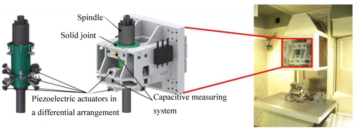
The advantage of the selected system results from the parallel kinematic arrangement with eight actuators (Figure 1). For simplified considerations, it is possible to initially only use individual degrees of movement freedom and the coupled degrees of processing freedom. This means that the results of the research can be transferred not only to the simple single-axis systems, but can also be used for very complex systems with several degrees of freedom and couplings.

The methods and algorithms to be implemented should essentially be based on the measurement data. For a later application in production, this method has the advantage, that the models, which combine data-learning technics with dynamics analyse are more widely accepted than methods based “purely” on simulation data. However, in this case, the final model will have high complexity and cannot be used with different kinds of machines. That’s why on this step of the research the simplification of the dynamic’s simulation will be researched. Ideally the whole dynamics must be in the form of a “black-box” and modelling should be with minimal error even without any knowledge about properties of the machine and its dynamics.

The dynamics overviews will be used only for supporting role in model creating stage. This will make it possible to concentrate on essentials first and to exclude other sources of error or to be able to localize errors later on the real systems better.

In order to be able to calculate the control data in advance, a suitable mathematical–physical relationship in the form of a model should be derived from the component measurement data and the specified target geometry. Since the actual data are obtained directly on the component, the influence of the tool, component and machining process is also recorded indirectly. With a pure system identification based on measurement data of the transfer functions of the kinematic axes, these would not be included.

To implement the intended goal, the tested approaches from experimental system identification, the area of learning control processes or machine learning should be used and these should be adapted accordingly.

This article is an overview of simplifying the model, taking into account the importance of the main parameters of the dynamics and a search for mathematical techniques to “ignore” these parameters with minimal error.

2. State of Research

In the industrial environment of the machine tool, piezoceramic actuator systems have so far been used in two main areas of application. On the one hand, this is the ultrasound-assisted processing of brittle hard materials or composite materials. By superimposing the rotary motion of the tool with a high-frequency vibration in the axial direction, it is possible to process complex materials more efficiently with increasing the process quality. For this, as example, DMG-Mori launched the Ultrasonic machine series [2]. On the other hand, the Fast Tool Servos (FTS) with monolithic diamond cutting edges (example from Kinetic Ceramics [3]) are used to process the inner or outer contour of rotating parts.

Apart from these two fields of application, piezoelectric actuator systems have not yet been able to establish themselves in the area of the machine tools. The causes for this are multifarious. However, many potential applications have in common that the active additional systems cannot take advantage of the dynamic advantages of the piezoelectric actuators due to the system (mechanical restrictions or position of natural frequencies). This disadvantage does not apply to ultrasound-assisted machining and FTS-systems. The advantage of ultrasonic vibration systems is that they operate in their design-based resonance and that exact and controlled positioning is not necessary. Due to the design, a very high mechanical natural frequency can be achieved with the FTS systems (1 kHz to 5 kHz) [3,4,5]. The systems are uniaxial, simple and only a very small part, usually the tool with cutting edge, is moved. This makes possible to achieve a very high bandwidth with these systems.

However, if larger parts have to be moved in relation to the positioning system, mechanical restrictions come into play that severely limit the maximum possible controller range. For example, cross-coupling between the axes [6] or the moving workpiece [7] mean, that the effective controller bandwidth is often significantly smaller. In [8], for example, a piezo-kinematic tool with a natural frequency of 1.1 kHz is presented, the bandwidth of which, depending on the control algorithm used, is only 300, 450 or 520 Hz. The piezoelectric tool for revolution systems presented by Altintas in [5] can realize a bandwidth of 200 Hz using “sliding mode control”, while the natural frequency of the tool in the machining direction is 3.2 kHz. The manufacturer of physics instruments also specifies the first natural frequency in the range of, for example, 400 Hz to 800 Hz (series P-612 and P-62X) for its piezoelectric nano-positioning systems, which already drops to 200 Hz to 300 Hz with a load mass of 100 g [9]. The performance and the advantages of piezoelectric actuators with regard to dynamics can therefore not be exploited due to the restrictions of the overall system, or the necessary positioning or manufacturing accuracy can no longer be guaranteed.

In the course of numerous preparatory works, several additional piezoelectric actuator systems for machine tools have already been developed and their potential for process optimization has been examined. In addition to systems for vibration compensation and increased dynamics in the power train [10] of machine tools, two active spindle systems [6,11], an active honing tool [12] and a piezoelectric cross table [12] for the fine positioning of the cutting edge or workpiece were developed, which can be used for the targeted structuring and contouring of surfaces or bores. The use of PI controllers [13] and compensation controllers was also examined using the production of typical cloverleaf geometries. However, sufficient stability of the control loop and accuracy could only be achieved significantly below 1000 rpm. Production-relevant parameters, for example for the machining of gray cast iron, are sometimes above 4000 rpm in order to achieve the required surface quality. The cycle time also plays an important role in the economy of the machining process, which in turn determines the feed to be used and thus the speed. A reduction in the machining speed or adjustment of the cycle times just to meet the bandwidth of the controller is therefore not acceptable. The advantages of piezoelectric actuators cannot therefore be exploited in controlled operation.

3. Model Build and Simplification

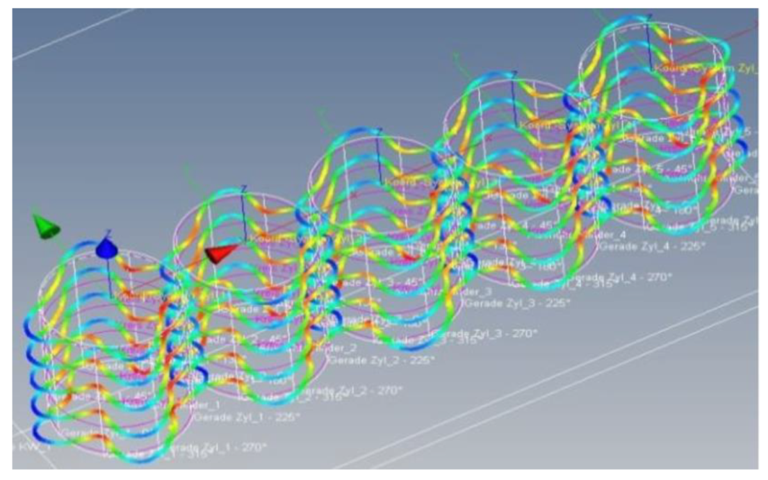
Since the piezoelectric kinematics have a very good repeat accuracy (Figure 2), an iterative process has therefore been developed in further investigations. Figure 2 represents output data of tactile micrometer. The tool with a cutting edge moves along Z-axis from top (0 mm) to bottom (120 or 150 mm) of the cylinder. After drilling of the cylinder is complete, the tool goes up and moves to the right to the next cylinder. In previous projects it was investigated, that this process has a high repeatability and with the same input signals with the same cylinder materials, the shape will be repeated at any position of the tool along the X-axis (left-right).

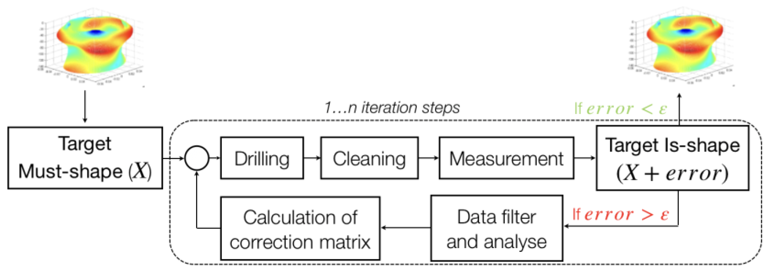
From control engineering, the method of “iterative learning control” (ILC) is also known [14,15] and can therefore also be used to describe the general procedure. By using ILC, the existing error of the drive signal of a periodic signal is corrected after the passage of a period. For the subsequent iterative production process carried out, the period would therefore amount to several hours and be carried out “manually”. The schematic procedure is shown in Figure 3.

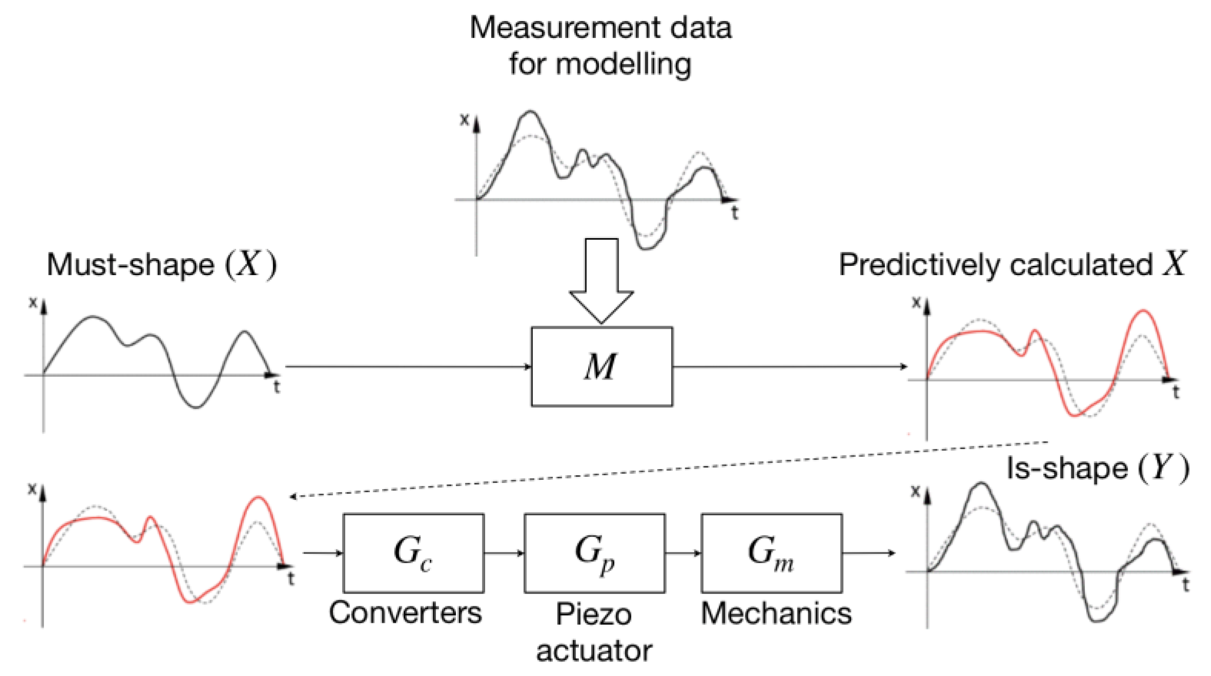
It is relevant to create such a model with the help of which it would be possible to predict the dynamics of a given system, thereby getting rid of this iterative process (Figure 4).

Having X and using the model, the input signal can be found, applying which Y = X output will be received given the fluctuations and dynamics errors.

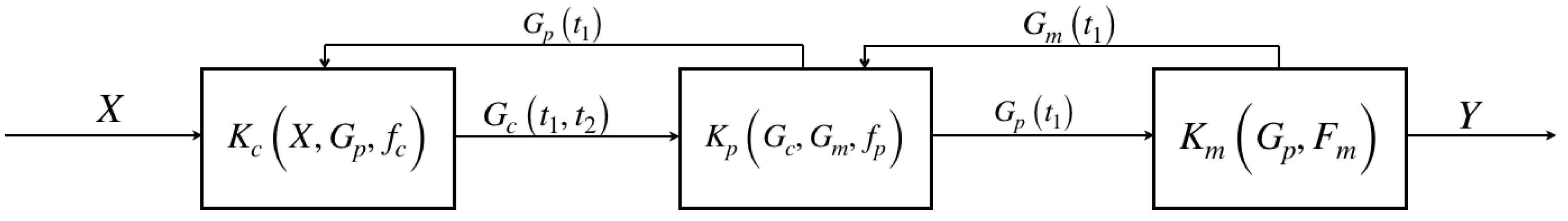
In an open-type system without feedback, the dependence between real output (Y) and given/control (X) will be as follows:

$$Y=G\left(G_c,G_p,G_m\right)$$

(1)

• $G_c\left(X,G_p,K_c\right)$ —power circuit dynamics, which depends on the control signal X, the inverse dynamics of the piezoelectric actuators G_p, and the own converter static coefficients K_c;
• $G_p\left(G_c,G_m,K_p\right)$ —piezoelectric actuators dynamics, which depends on the power circuit dynamics G_c, mechanics dynamics G_m, and the own piezoelectric actuators static coefficients;
• $G_m\left(G_p,F_m\left(Y\right),K_m\right)$ —mechanics dynamics which depends on the piezoelectric actuator’s dynamics G_p, processed material reaction F_b, which depends on the output form Y, and the own mechanic static coefficients K_m.

In expanded form, this function is represented as:

$$Y=G\left(G_c\left(X,G_p,K_c\right),G_p\left(G_c,G_m,K_p\right),G_m\left(G_p,F_m\left(Y\right),K_m\right)\right)$$

(2)

The complete model is shown in Figure 5.

This function has interchangeable parameters, where one parameter depends on the second in a closed loop. In order to remove the cycle, it is necessary to discretize the function. Since control is implemented by setting 721 control points per spindle revolution, the discretization can also be done with the same step.

$$Y\left[n\right]=G_k\left(Y\left[n-1\right],F_m,K_k,f_p,G_c\left(X\left[n\right],Z_p\left(F,\vartheta ,S\right),f_c\right)\right)$$

(3)

n = 1, 2, …, 721.

Since $\Delta Y=Y\left[n\right]-Y\left[n-1\right]$ is extremely small over an extremely small period of time for changing mechanics and piezoelectric dynamics, it can be used as the piezoelectric actuator’s length and for calculations in the moment. Then the static coefficients of the entire kinematics can be taken out in a separate matrix, both mechanics and piezoelectric actuator functions can be combined into the kinematic function. To describe the dynamics of piezoelectric actuators in a mechanical circuit, it is enough to analyze the frequency of the mechanical oscillations. The dynamics of the converter depends on the control signal, the piezoelectric actuator impedance, and the control frequency. The oscillation form of a piezoelectric actuator in steady-state modes has the same frequency as the frequency of the converter, but it is out of phase.

Open-type system dynamics can be represented in vector form as

$$\Delta \overrightarrow{G}=\overrightarrow{AG}\left[n\right]+\overrightarrow{BF}\left[n\right]$$

(4)

G—dynamics, F—reaction or influence, A—coefficient matrix, and B—influence matrix.

The speed of the parameters G[n] and F[n] of the piezoelectric actuators can approximately match the speed of the parameters of the power circuit. However, the speed of the state variables A and B of mechanical and electrical circuits is variable. Since in this function it is necessary to use two or more different lengths of the integration steps, this function needs to be divided or simplified.

Piezoelectric actuator state change in $G\left(G_p\left[n\right],G_m\left[n\right]\right)$ system is

$$\Delta G_p=A_p{G}_p\left[n\right]+B_p{F}_m\left(G_m\left[n\right]\right)$$

(5)

As in (3), mechanical processes in the spindle and mechanical part of the electro-mechanical processes in piezoelectric actuators are approximately proportional in speed and can be merged into a kinematic model, which contains the functions of the piezoelectric actuators and mechanics, as well as the reaction of the processed material:

$$\Delta G_k=A_k{G}_k\left[n\right]$$

(6)

Kinematics state change in $G\left(G_k\left[n\right],G_c\left[n\right]\right)$:

$$\Delta G_k=A_k{G}_k\left[n_k\right]+B_{k}F\left(G_c\left[n_c\right]\right)$$

(7)

The effect of the power circuit on the kinematics is described as an external action with variable parameters. Since the speed of the dynamic of these systems will be different, the whole system will have a high coefficient of rigidity.

Power circuit’s state change in $G\left(G_k\left[n\right],G_c\left[n\right]\right)$:

$$\Delta G_c=A_c\left(G_k\left[n_k\right]\right)G_c\left[n_c\right]+B_c$$

(8)

As a reactive load with variable values, kinematics affects the parameters of the electric circuit, thereby changing the value of the coefficient matrix.

The solution to the problem of system stiffness is a separation of values with different integration steps.

Then using the diacoptics [16] principles for system of equations:

$$\begin{array}{l}\{\begin{array}{l}\Delta G_k=A_k{G}_k\left[n_k\right]+B_{k}F\hfill \\ \Delta G_c=A_c{G}_c\left[n_c\right]+B_c\hfill \end{array}\hfill \\ F\to F\left(G_c\left[n_c\right]\right)=F\left(G_c\left[m_c{h}_c\right]\right)=U_p\left[m_c{h}_c\right]\hfill \\ A_c\to A_c\left(G_k\left[n_k\right]\right)=A_c\left[n_k-1\right]+\Delta A_c\left(G_k\left[m_k{h}_k\right]\right)=A_{c_{const}}+\Delta A_c\left[m_k{h}_k\right]\hfill \end{array}$$

(9)

U_p—piezoelectric actuator voltage; m—count of the step h.

With this approach, the kinematics model can be built on the interval of electric circuit structure constancy with step h and the converters model can be built on the interval of kinematic structure constancy with step h_k.

The system of equations with communication equations is presented in Figure 6.

The complexity of this approach lies in the fact that it is rather difficult to calculate the intervals of constancy to satisfy the stability conditions of both systems together. Sufficient stability conditions can be calculated only for real values of the characteristic equation roots of the entire system. Using Rayleigh’s formulas, approximate stability zones of this method can be calculated for complex values.

These minimal requirements must be met:

• For stability: h_k/h_c ≈ λ_c/λ_k, since the roots of the characteristic equation directly depend on the speed of the processes of a particular model.
• Sensitivity characteristic: S_λ(i)/ΔG→0.

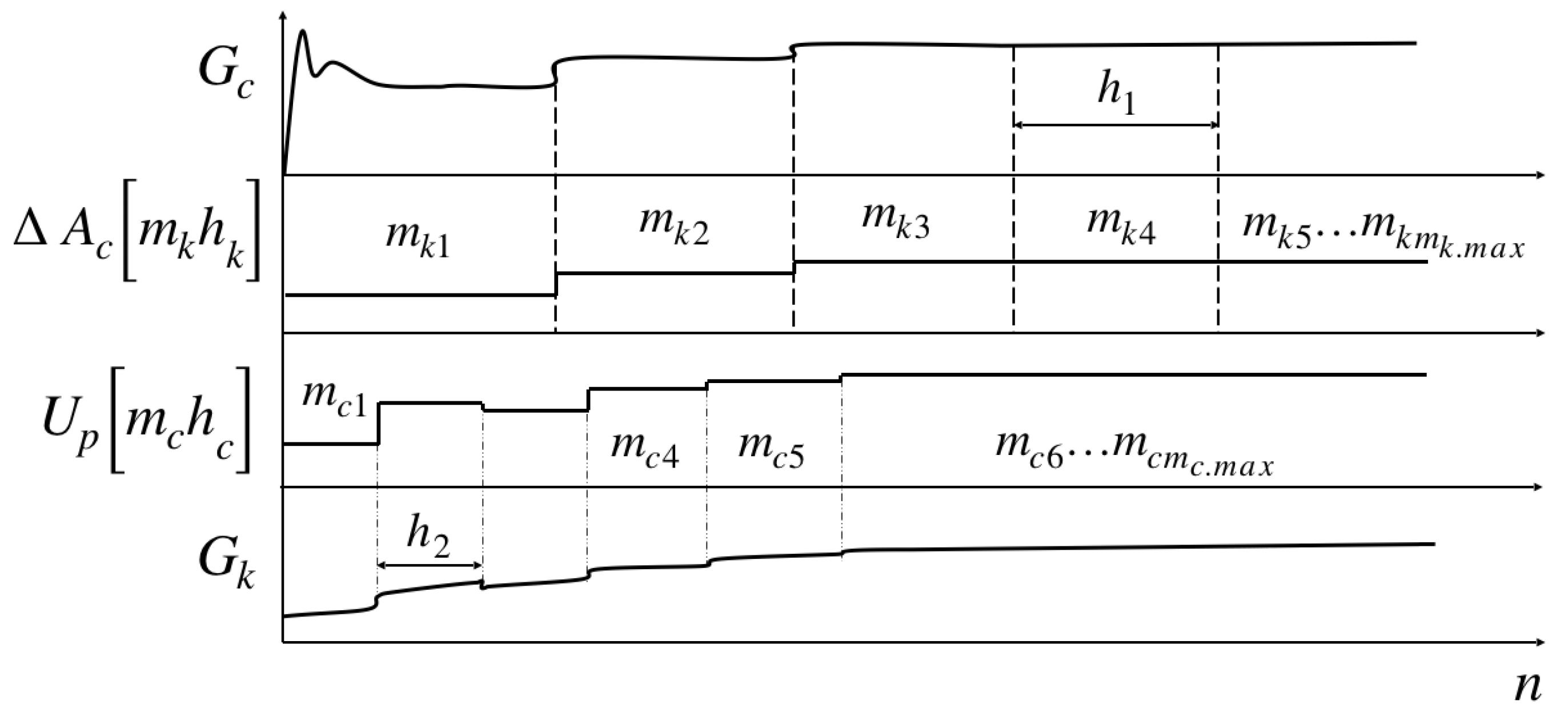
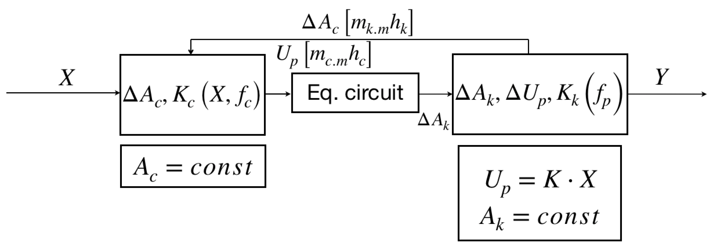
The model takes the form as in Figure 7.

If h_c includes the interval $n_1\dots n_{m_c}$ (where $h_c=n_{m_c}-1$), then $U_p\left[n_1\right]\dots U_p\left[n_{m_c}\right]=U_p\left[n_1\right]=U_p\left[m_{c.m}{h}_c\right]$ is constant during the whole step h_c and is equal to the value at the first point $n_1$. If $n_{m_c+1}$ belongs to the next step $\left(m_c+1\right)h$ then U_p becomes the new constant value at the new step $U_p\left[m_{c.m}{h}_c\right]=U_p\left[n_{m_c+1}\right]$. In exactly the same way, $\Delta A_c\left[m_{k.m}{h}_k\right]$ can be calculated.

$U_p\left[m_{c.m}{h}_c\right]$ includes gained given control signal U_p = K⋅X and fluctuations caused by the dynamics of the power circuit and parasitic feedback of the piezoelectric element ΔU_p which are constant on the interval h_c and therefore can be separated from the signal U_p.

Kinematics coefficient matrix has the following form:

$$A_{k+}=\left|\begin{array}{ccc}0& 1& 0\\ -\frac{K_e}{m}& -\frac{K_d}{m}& \frac{K_u}{m}\\ 0& -\frac{K_{dr}}{C_p}& -\frac{1}{R{C}_p}\end{array}\right|, A_{k0}=\left|\begin{array}{ccc}0& 1& 0\\ -\frac{K_e}{m}& -\frac{K_d}{m}& \frac{K_u}{m}\\ 0& -\frac{K_{dr}}{C_p}& 0\end{array}\right|$$

(10)

K_e—elasticity coefficient, K_d—damping coefficient, K_u—reverse piezoelectric effect, K_dr—direct piezoelectric effect, m—weight, A_k+—plus or minus control (with external power source), A_k0—null control (without external power source, only reactive elements).

All values except the piezoelectric element capacitance C_p can be taken as constant given the operating modes of the device. To simplify this model, it is necessary to separate constant values from variable ones.

The equation characterizing the movement of kinematics (Is-value Y(t)) can be set in the following form:

$$m\frac{{\mathrm{d}}^{2}Y}{\mathrm{d}t}+K_d\frac{\mathrm{d}Y}{\mathrm{d}t}+K_{e}Y=F$$

(11)

F—force

Given that dY/dt = ϑ, Equation (11) can be written as:

$$m\frac{\mathrm{d}\vartheta }{\mathrm{d}t}+K_d\vartheta +K_e\int \vartheta \mathrm{d}t=F$$

(12)

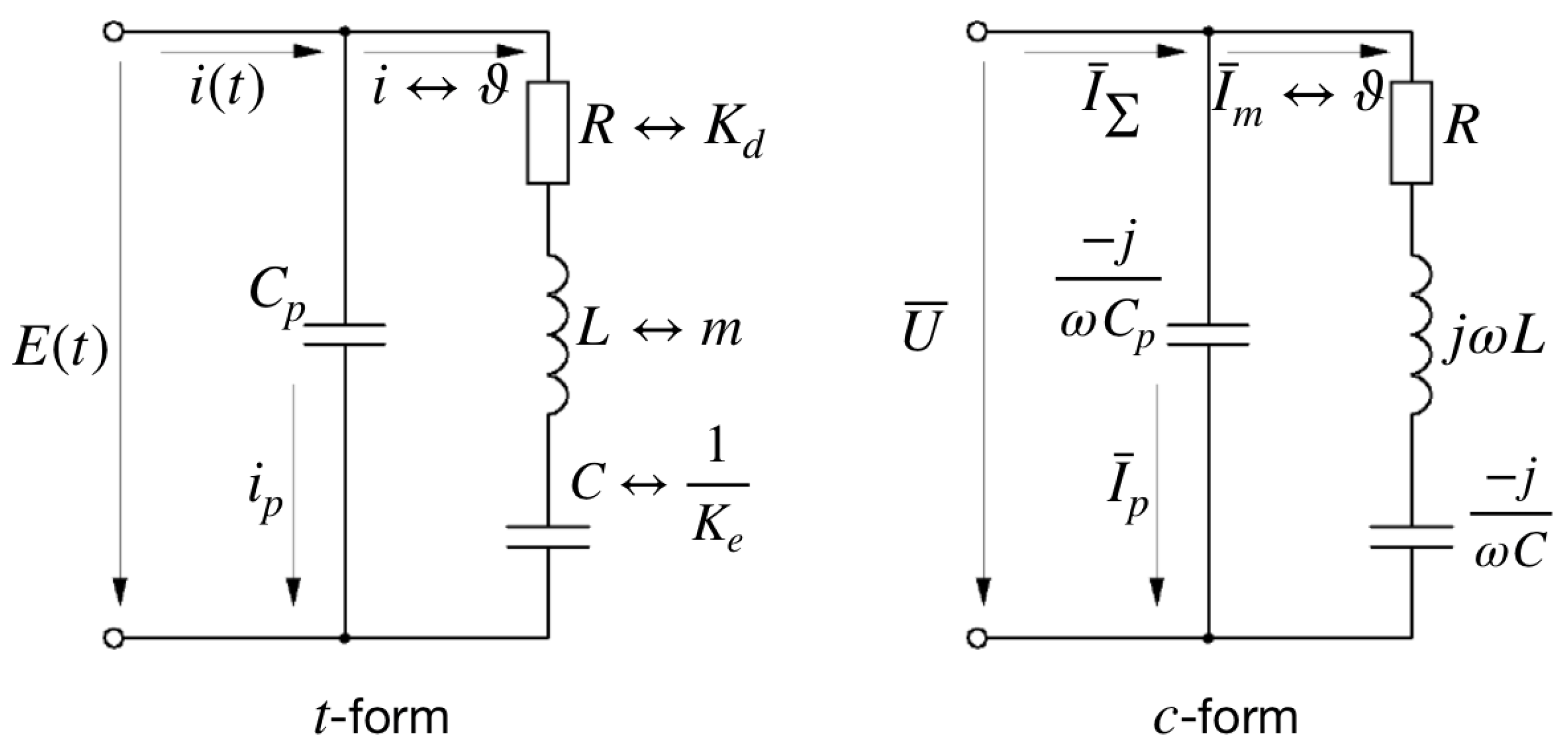
The equation for an electric circuit:

$$L\frac{\mathrm{d}i}{\mathrm{d}t}+Ri+\frac{1}{C}\int i\mathrm{d}t=E$$

(13)

Comparing (12) and (13) an equivalent electrical circuit can be created (Figure 8). Values F∼E, ϑ∼i, m∼L, K_d∼R, K_e∼1/C. During resonance: U/I = F/ϑ.

Piezoelectric element capacity:

$$C_p=\frac{\epsilon {\epsilon }_0{l}_1{l}_2}{l_3}\left(1-k_{31}^2\right)$$

(14)

k₃₁—electromechanical coupling coefficient.

In the case of this equivalent replacement, the frequency response formula will look like:

$$G_k\left(\omega \right)=\sqrt{\frac{{\left(-C_{p}RC{\omega }^2\right)}^2+{\left(\left(C_p+C\right)\omega -C_{p}LC{\omega }^3\right)}^2}{{\left(1-LC{\omega }^2\right)}^2+{\left(RC\omega \right)}^2}}$$

(15)

and phase-frequency characteristic:

$$\phi \left(\omega \right)=\arctan \frac{\left(C_p+C\right)-C_{p}LC{\omega }^2}{-C_{p}RC\omega }-\arctan \frac{RC\omega }{1-LC{\omega }^2}$$

(16)

The model takes the next form (Figure 9):

The complete system dynamics G_ck with complete coefficient matrix A_ck in this case will look like [17]:

for (+) or (−) control:

$$G_{ck}\left(\left(n+1\right)h\right)=e^{A_{ck}Dh}{G}_{ck}\left(nh\right)+A^{-1}\left(e^{A_{ck}Dh}-I\right)B$$

(17)

for (0) control

$$G_{ck}\left(\left(n+1\right)h\right)=e^{A_{ck}\left(1-D\right)h}{G}_{ck}\left(nh\right)$$

(18)

D—duration of (+) control.

At this step, assumptions were made that, having identified and calculated the most influential parameters of the dynamics of the piezoelectric element, the coefficient matrix can be represented as a constant matrix influenced by the function of influence:

$$A=A_{const}+G_A\left[n\right]$$

(19)

Having enough experimental data, it is possible to find the function of G_A using regression analysis or machine learning to represent the coefficient matrix of mechanics as a constant.

Same way as in (19), voltage fluctuations can be represented as a function, taken from experimental data and processed by regression or machine learning tools:

$$U_p=K·X+G_U\left[n\right]$$

(20)

or if provide the model as a holistic system, G_U [n] can be represented through K⋅X and G_A [n].

The model takes the form as in Figure 10:

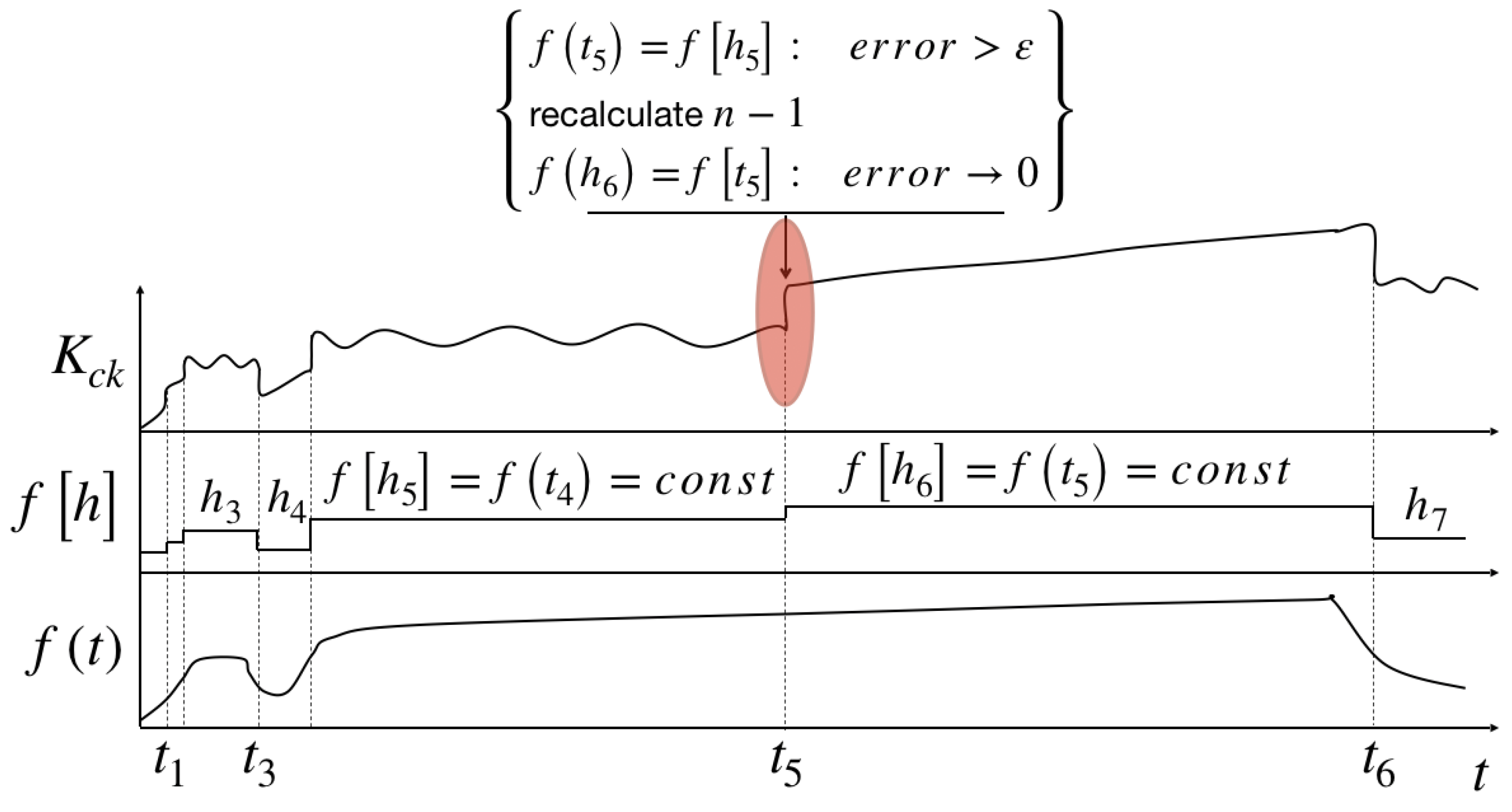
The frequency depends on the drilling shape which is specified in the control signal $X$. For basic symmetrical shapes (cylinder, three leaf, six leaf), the frequency will be constant during whole drill revolution. For non-symmetrical shapes, the frequency will be changed during revolution. Finding the frequency ranges, within which the frequency changes have influence for $K_{ck}$ mode change less, than the permissible error (Figure 11), the model can be simplified even more.

$$\{\begin{array}{l}f\left[h_1\right]=f\left[t_1\right] \parallel n=1,\dots ,m-1:error<\epsilon \hfill \\ f\left[h_2\right]=f\left[t_m\right] \parallel n=m,\dots ,k-1:error<\epsilon \hfill \\ f\left[h_3\right]=f\left[t_k\right] \parallel \dots \hfill \end{array}$$

(21)

Since the frequency has a constant value at constancy intervals, the difference between f_c and f_p as well as the phase shift between power electrical circuit and kinematics can be described linearly.

The state of the entire system (Figure 12) can be described as:

$$\Delta Y=K_{ck}\left(f\left[h\right]Y\left[n-1\right]+G_{ck}\left(A,X\right)\right)$$

(22)

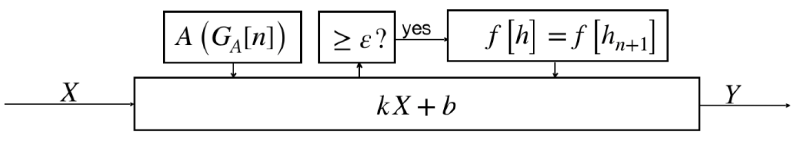
This model allows using data from previous experiments and completing the database of A(G_A [n]), create learning system which can transform the given data (X) to real output signal (Y) as a linear function Y = kX + b, where k represents dynamic of the whole system and b represents the shape of the drilling.

4. Implementation of the Method

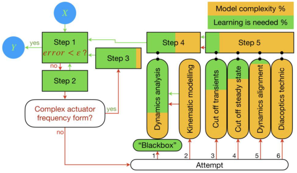
Processing of the complex shape drilling can be divided into five steps. The larger the step number, the more complex of a model must be used and the less experimental data usage is necessary. After necessary operations are completed, the model is returning to a lower step number.

Step 1. Assumption: all dynamics can be divided into constant form and function of changes. Then the real form depends linear on the given form with constant coefficient plus drilling shape function $Y=kX+b$.

Step 2. If the error of Step 1 exceeds the permissible value, there can be used some hardware implementations: Plus-minus control can be used instead of plus-null control to transform the non-symmetric shape to a symmetric shape or to decrease the necessary actuator frequency to its half. Additionally, experimental tests found that using $0.7U_{p.max}$ greatly improves the shape.

Step 3. Assumption: dynamic is constant on different frequency bands.

Step 4. In a first attempt, the whole dynamic except the piezoelectric actuator is a “black box” built by analysis or machine learning based on experimental data. If this method does not satisfy the error requirements, in a next attempt the whole actuator dynamic calculation takes place.

Step 5. If the actuator dynamic calculation still does not satisfies the error requirements, there are 4 attempts for modeling the power circuit: transients and steady state operation modes replaced by function from experimental data, regression methods, and if no previous attempt satisfy the error requirements, then full model calculation using diacoptics methods (system state equations with functions of communication).

The block diagram in Figure 13 describes the full functioning of the model.

The next step is the experimental drilling with such shapes, an analysis of which will be used for building a function that will allow simulating all possible shapes using a step no higher than Step 3.

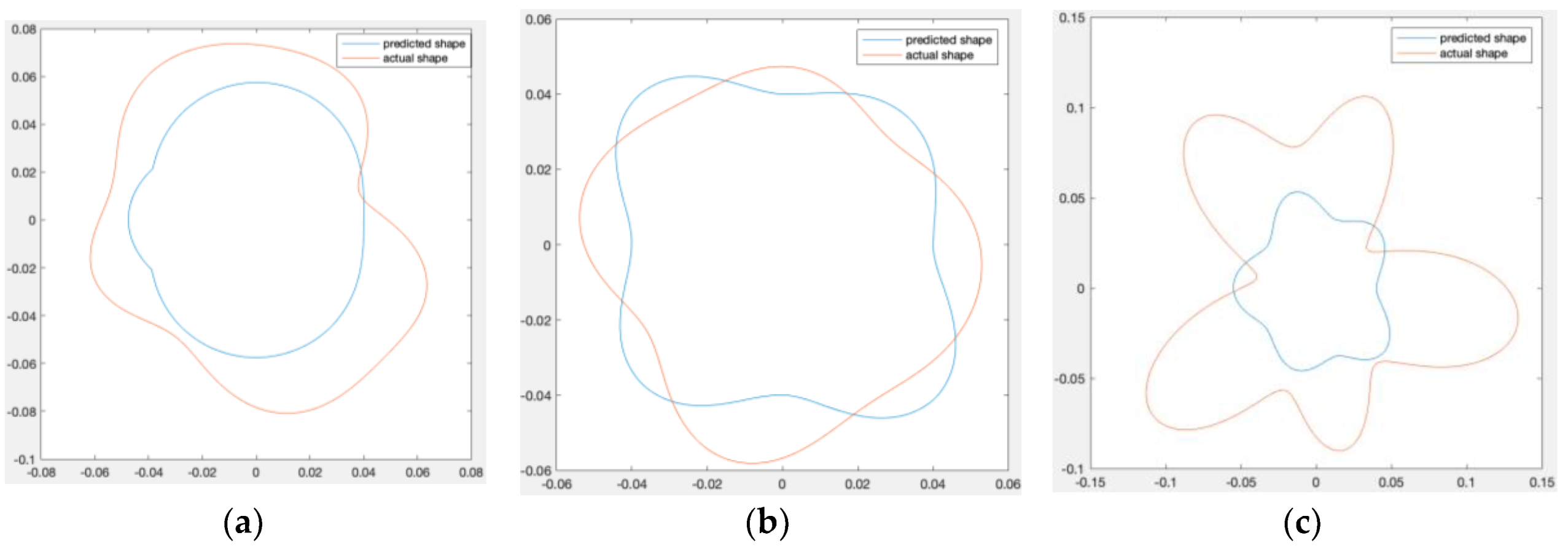
Of course, with a complete calculation of the dynamics it is possible to predict such a control signal in which the shape of the bore will be as accurate as possible. But such a technique cannot be transferred to another system, as well as cannot be used in industry with frequent changes in shapes, workpiece materials, cutting edges and processing speeds. Even when working with the same material, there are non-lineal errors on the part of the dynamics, resonances during movement from top to bottom, natural resonances of the machine at different speeds of revolution, vibration of the table, differences in response of the piezoelectric elements by processing different shapes.

Figure 14a shows the shape with three pulses per revolution on Z = 40 mm. A small phase shift is observed, as well as an uneven electrical resonance of piezoelectric elements located along the X- and Y-axis, which distorts the shape and increases the processing amplitude by 2.5 times (excluding the initial cylinder diameter). Figure 14b shows the shape inside of the same cylinder but on Z = 80 mm. There are no resonances, and dynamics is linear, and the actual shape has minimal error compared to predicted. But there is significant increased phase shift (almost 45°) because of increasing of pulse amount per revolution. Figure 14c shows the shape inside of the same cylinder but on Z = 100 mm. That is the worst position and shape combination for the processing at 4000 revolutions per minute. The electrical resonance of actuators is combined with mechanical vibrations and self-resonance of the machine creates almost the same amplitudes in the X- and Y-axes, which does not distort the shape, but increases the processing amplitude by a factor of 7.2. Phase shift is increased again to almost 90°.

This shows the lack of conventional machine learning methods for these processes due to non-linear changes in dynamics during the processing of even the sae cylinder. Pre-processing in air before any new shape combination without a cylinder may help to improve the processing, but it takes time and in industrial mass production is unacceptable.

Taking the worst scenario of processing of this cylinder, the frequency intervals of states can be learnt. Additionally, the pulse frequency can be double decreased by turning X and Y actuators through time. This allows to get rid of the phase shift (Figure 15a). The mechanical resonance can be decreased by separating revolution speed on different constancy intervals (step 3, the speed varies from 4000 to 6000 rpm Figure 15b) or using the speed in close range to self-resonance speed but with increasing actuator force (step 5, increasing voltage, switch from “+ 0” control to “+ −” control with a sharp retraction of the cutting edge after touching, parallel connection of 3µF capacitors to each piezoelectric actuator, taking into account the capacitance of the actuator 0.8µF and voltage range 200−800V per actuator—Figure 15c). The third option is slightly more accurate that the second. However, at the same time, it is more universal for all shapes.

At this stage, there is still a very high percentage of the dynamic’s calculations, which does not correspond to the condition of compatibility with a high number of machines of the same type or same machine with different processes or cylinder materials.

The next stage of the research involves model training to identify dynamics without directly knowing what dynamics of the process are currently present. The techniques of this training imply further investigation of vibration using a laser vibrometer, parallel experiments with harmonic analysis, noise reduction and pulse width suppression of parasitic harmonics of the process. The end results mean processing with “black box” without any knowing about process dynamics.

5. Conclusions

To get rid of iteration steps during shape drilling, the model representing the drilling system dynamic was created. With optimization goals, as well as with the goal to use the model on different systems without access to the parameters of such systems but only with access to previous experimental data, the model was simplified for different system-knowledge levels and the amount of previous experimental data. The method was implemented for a different usage of the drilling system parameters and experimental data. This method is planned as self-learning, that is why the model complexity is divided in steps from Step 1 to Step 5. Even if the model does not have experimental data and operates using Step 5, after obtaining the data, the step number will be decreased.

The machine learning tools can be created using regression analysis of the drilling systems output combined with an analysis of the systems full model represented by Steps 5 and 4.

The cons of the simplification are the dependency on the workpiece material. This means that the experimental data have to be collected for each individual material. The advantage of the models is that the drilling system can be represented as “black box” without knowing most parameters or any parameters at all.