Article

Analysis of the Influence of Suspension Actuator Limitations on Ride Comfort in Passenger Cars Using Model Predictive Control

1
Department of Mechanical Engineering, Institute of Automotive Technology, Technical University of Munich, Boltzmannstr. 15, 85748 Garching, Germany
2
Bayerische Motoren Werke AG, Petuelring 130, 80788 München, Germany
*
Author to whom correspondence should be addressed.
Actuators 2020, 9(3), 77; https://doi.org/10.3390/act9030077
Submission received: 27 July 2020 / Revised: 12 August 2020 / Accepted: 20 August 2020 / Published: 25 August 2020
(This article belongs to the Section Actuators for Land Transport)

Abstract

:
Active suspension systems help to deliver superior ride comfort and can be used to resolve the objective conflict between ride comfort and road-holding. Currently, there exists no method for analyzing the influence of actuator limitations, such as maximum force and maximum rate of change, on the achievable ride comfort. This research paper presents a method that is capable of doing this. It uses model predictive control to eliminate the influence of feedback controller performance and to integrate both actuator limitations and necessary constraints on dynamic wheel-load variation and suspension travel. Various scenarios are simulated, such as driving over a speed bump and inner city driving, as well as driving on a country road and motorway driving, using a state-of-the-art quarter-car model, parameterized for a luxury class vehicle. It is analyzed how comfort, or in one scenario road-holding, can be improved with consideration for the actuator limitations. The results indicate that actuator rate limitation has a strong influence on vertical vehicle dynamics control system performance, and that relatively small maximum forces of around 1000 to 2000 N are sufficient to successfully reject disturbances from road irregularities, provided the actuator is capable of supplying the forces at a sufficiently high rate of change.

1. Introduction

Together, automated and autonomous driving, and new propulsion technologies, make up one of the biggest research fields in the automotive industry. The switch in roles from driver to passenger, offers both opportunities and pitfalls for the near future, at least in some scenarios. Many characteristics of today’s road vehicles are designed to please the driver, as he or she is usually the customer. A typical development methodology is the so called V-Model [1,2], which is defined for mechatronic systems in VDI 2206 [3]. It prescribes a framework for development according to requirements defined for the product, subsystem and component levels. Vehicles thus developed must fulfill all requirements prescribed by law. In automotive software development, ISO 26262 [4] is applied to secure functional safety. Other requirements are more difficult to define, as they are dependent on many internal and external factors, such as customer demand, market strategy, self-set quality standards and price targets. Having set these vehicle-specific requirements on product level, they need to be broken down to subsystem and component level. In order to do this, it is necessary to understand the interdependency between subsystem performance and product performance. Objective measures for quantifying subsystem and product performance are also required. In the case of vehicle dynamics and suspension development for passenger cars, these matters are well-understood thanks to the decades of experience and research carried out by the manufactures and universities [5,6]. However, this all changes when it comes to automated and autonomous vehicles, as there is a lack of accumulated experience, and it is not clear how the customer preferences might change. Previous studies of the authors indicate a demand for increased comfort during an automated drive [7,8,9]. This is in conflict with traditional driving-dynamics requirements where requirements placed on longitudinal and lateral dynamics generally have priority over comfort, except in the case of luxury vehicles. Furthermore, an ideal vehicle offering automated driving functionality must be able to fulfill both automated and non-automated requirements in the best possible manner. Active suspension systems help to resolve this conflict, because they can be tuned to suit the different objectives for each driving mode. However, the precise relationship between active suspension system actuator performance and comfort requirements at vehicle level are currently neither known nor understood, either in academia, or in the automotive industry. This research paper aims to close this research gap.

2. State of the Art

This section gives an overview of the current state of the art. Section 2.1 outlines vertical dynamics components their properties. Section 2.2 summarizes the objectification methods, while Section 2.3 and Section 2.4 provide an overview of passive, semi-active and active suspension systems and the current research into model predictive control in the context of vertical vehicle dynamics control. Finally, the gap in research is outlined in Section 2.5.

2.1. Suspension Components

The most important suspension components responsible for vertical vehicle dynamics are the springs and dampers, because it is these that have a major effect on the vehicle’s response to road irregularities and the reaction of the vehicle body to longitudinal and lateral accelerations. In combination with the mass of the vehicle body, the unsprung mass and the vertical stiffness of the tires, they define the frequency response of the vehicle in the range of 0 Hz to 20 Hz , which includes the body-mode eigenfrequency and the wheel-mode eigenfrequency. A more detailed description of this is given in Section 2.3. The general characteristics of passive and (semi-)active suspension springs and dampers will be explained in the following. Further information can be found in [10] (pp. 426–474).
The majority of main suspension springs fitted to road cars are either coil-, leaf- or air-type. Most active springs are air-type that can either switch between different airchambers to change suspension stiffness [11], or are controlled by air-pressure, mainly for ride-height adjustments in a low-bandwidth system [5]. An example of a high-bandwidth active spring system for controlling vehicle response is presented in [12]. Anti-roll bars (ARBs) are another type of springs fitted to vehicles, which connect the wheels (unsprung masses) of an axle to reduce body roll under lateral acceleration. The wheels are coupled, and any road-excitation from one side is transferred to the other. Active ARBs were developed as a means of providing roll stiffness under lateral acceleration, varying the roll-stiffness distribution, and minimizing coupling during straight-line driving. Examples of such systems are described in [13,14]. Besides springs, dampers are another integral part of a vehicle suspension. The design and working principles of suspension dampers are described in detail by Dixon [15]. As will be shown in Section 2.3, there is a conflict between ride comfort and road-holding. Electronically controlled, semi-active continuously variable dampers (CVD) were invented in an attempt to resolve this conflict. CVDs are usually magnetorheological [16] or electromechanical [17] systems. An implementation of a control system for CVDs is described in [18]. Active dampers are able to generate a desired force independently of the relative velocity of the damper, as introduced by Daimler [19]. An overview of passive, semi-active and active suspension dampers is given in [17]. There are also other active elements that cannot be directly classified as springs, dampers or ARBs, for example the fully active system developed by Lotus [20], or the system introduced by Ovalo and Audi, which can be installed in place of an ARB [21].

2.2. Objective Performance Measures

To quantify the performance of a vehicle suspension by simulation, it is necessary to define objective performance indicators that reflect human perception while driving a vehicle. In the context of this research, objective measures for vertical vehicle dynamics are needed. In terms of comfort, the main task of the suspension system is to insulate the vehicle occupant from road vibration induced by road irregularities. In order to quantify suspension performance, it is therefore necessary to quantify the vibration of the car body for a given road excitation, as it is this vibration that is transferred to the vehicle occupant through the seat, and it is also the output quantity that is solely dependent on the performance of the suspension system.
Human sense vibration through their visual, vestibular, somatic and auditory systems [22]. For measuring ride comfort in the context of vehicle suspension, the frequency range of interest is between 0 Hz to 20 Hz as stated in Section 2.1. As this is under the auditory threshold, the auditory system can be neglected in terms of suspension ride comfort, contrary to the field of noise, vibration and harshness. The mechanism of perception is still complex and there is a genuine difference between comfort and discomfort. According to Looze et al. [23] comfort has not yet been clearly defined, and the exact relationship between comfort and discomfort is still subject to debate. One theory is that comfort and discomfort are independent factors, and so a reduction in discomfort will not automatically yield an increase in comfort [24]. Furthermore, discomfort is a result of several factors, of which vibration is only one [25] (p. 44). The automotive term ’ride comfort’ is therefore imprecise, because it is usually suspension vibration discomfort that is the subject of analysis. Other influences, such as noise, can still have an unwanted effect on the subjective rating of suspension vibration discomfort in real vehicles [26].
There are three standards by which vibration discomfort is generally assessed, these being ISO 2631 [27], BS 6841 [28] and VDI 2057 [29]. They all apply the same method of using acceleration measurements to calculate a weighted root mean square (RMS) acceleration comfort value. Weighting is performed in the frequency domain with factors representing the frequency sensitivity. RMS acceleration values for each direction are calculated from the weighted signals and combined to a discomfort value using directional weighting factors representing the directional sensitivity of human perception. VDI 2057 [29] extends the method of ISO 2631 [27] for vibration containing shocks, while BS 6841 [28] uses slightly different frequency weighting factors. The authors performed a comparison of objectification methods for ride comfort. The results indicate, that the standardized methods are more robust and reliable than methods developed by other researchers [9]. All of these methods have in common that they objectify the ride comfort (vibration discomfort) as perceived by an untrained customer. Development engineers specializing in vertical vehicle dynamics have a different perception because of their background knowledge. They try to identify such different vibration phenomena as wheel hop, engine shake and copying and then correlate them to different parts and systems of the car. An overview of subjective development criteria is given in [30] (pp. 530–531).

2.3. Passive Suspension Systems

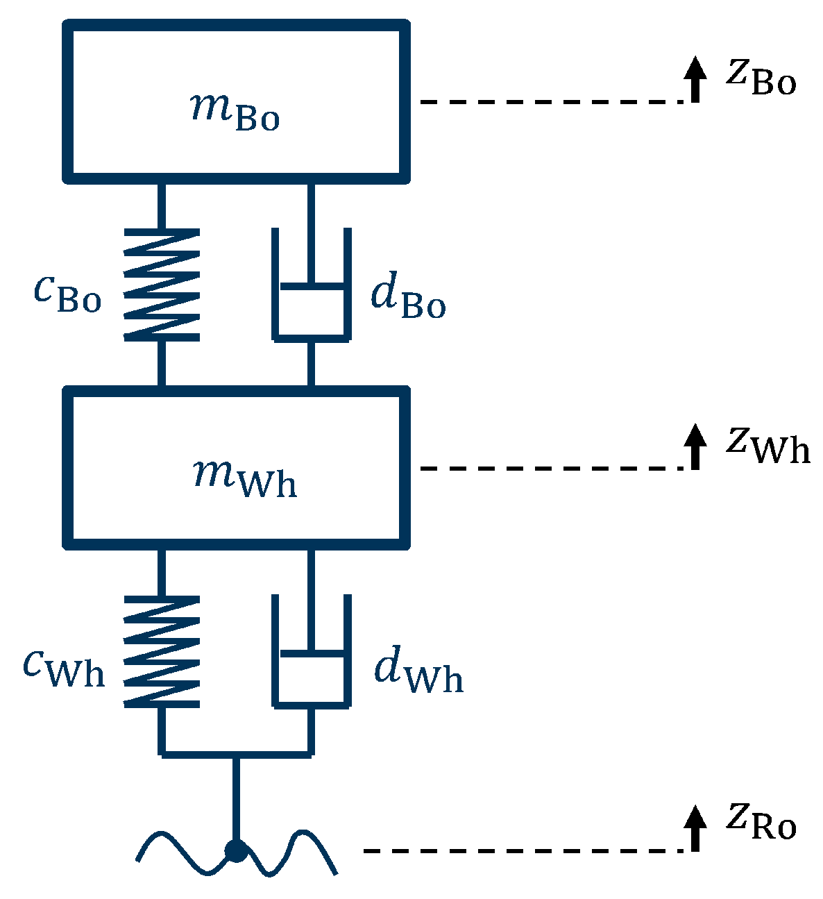
The quarter-vehicle model is used to describe the vertical dynamics of a passenger car. Here, the full vehicle is reduced to one corner and modeled as a two-mass spring-damper system, as illustrated in Figure 1. The mass m Bo represents the body, m Wh the unsprung mass. The two are connected by a spring and a damper representing the suspension stiffness c Bo and suspension damping d Bo . The wheel and the road are also connected by a spring and a damper, where c Wh is the tire stiffness and d Bo the tire damping. The displacements of the two masses and the road-profile are defined as z Bo , z Wh and z Ro . For a longitudinally symmetric vehicle, the quarter body mass is half of the corresponding axle weight, which itself depends on the front-to-rear weight distribution. The unsprung mass represents the mass of the wheel assembly. Tire stiffness is usually one magnitude higher than suspension stiffness, and tire damping is virtually negligible. The physical derivation of this model is described in [30] (pp. 295–299). This model has only two degrees of freedom and cannot model the pitch and roll behavior of vehicles. However, it is sufficient for describing the essential vertical dynamic behavior of a vehicle, which is characterized by the objective conflict between ride comfort, suspension travel and road-holding [31] (p. 112). The advantage of this model is its simplicity as a linear lumped parameter model, which makes it well suited to be used in control systems and for simulation purposes.
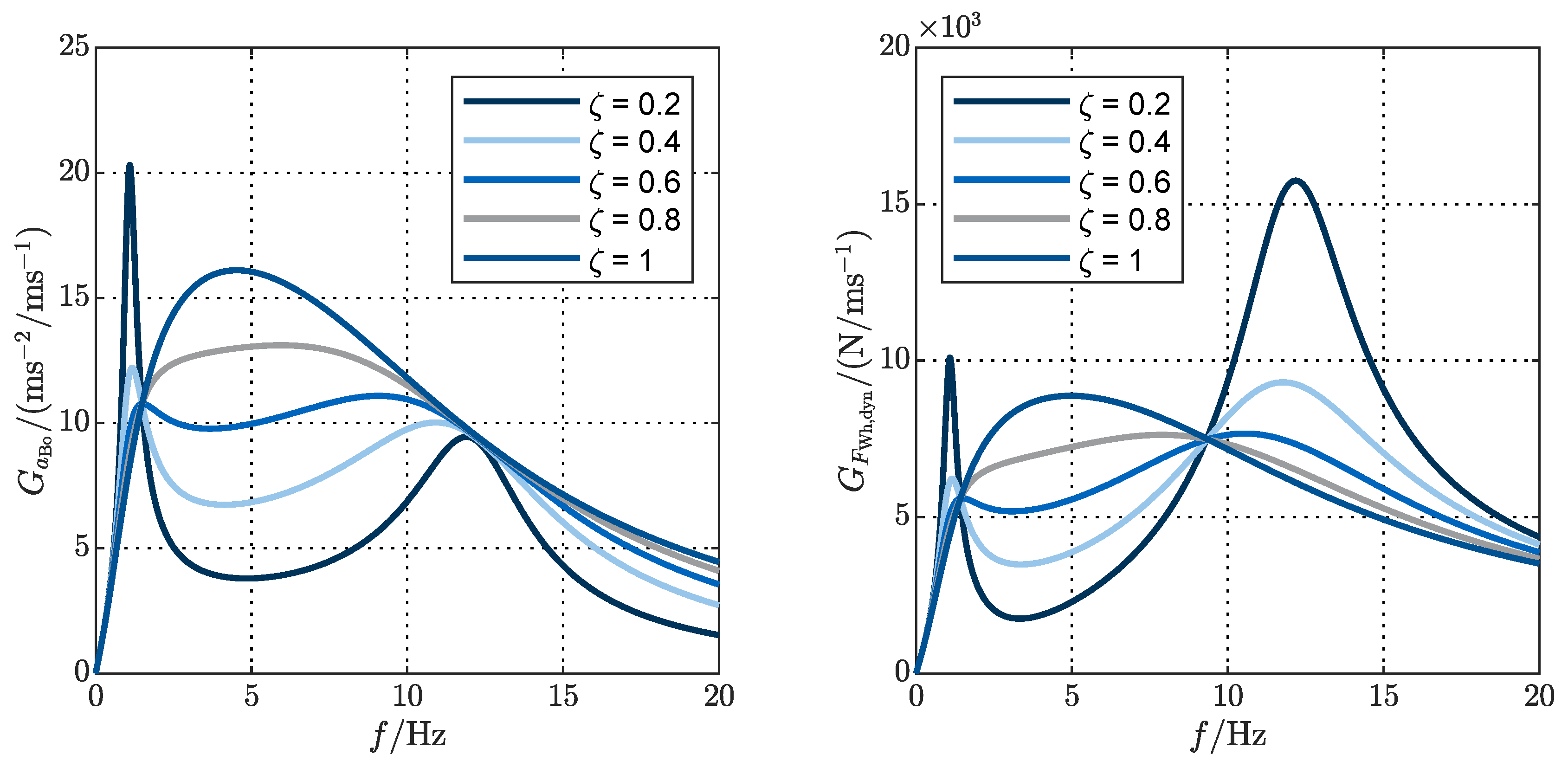
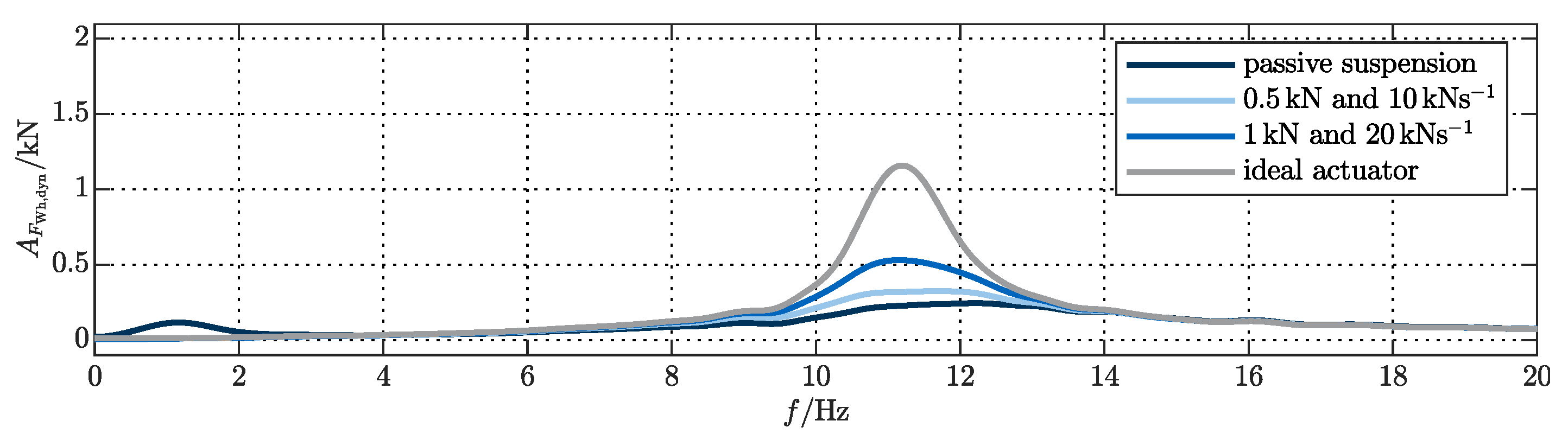
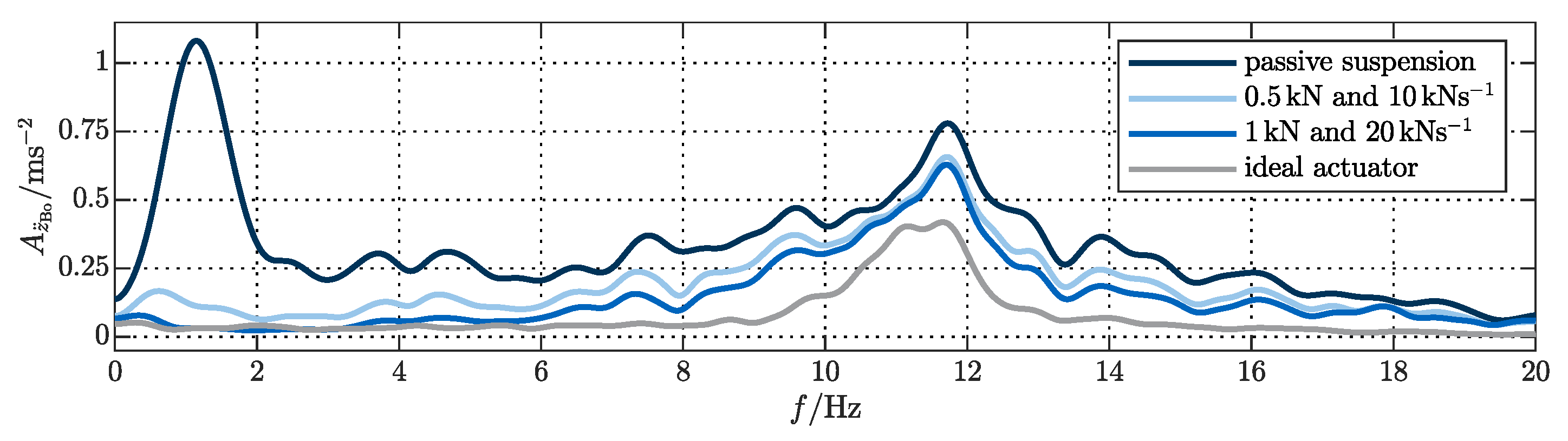
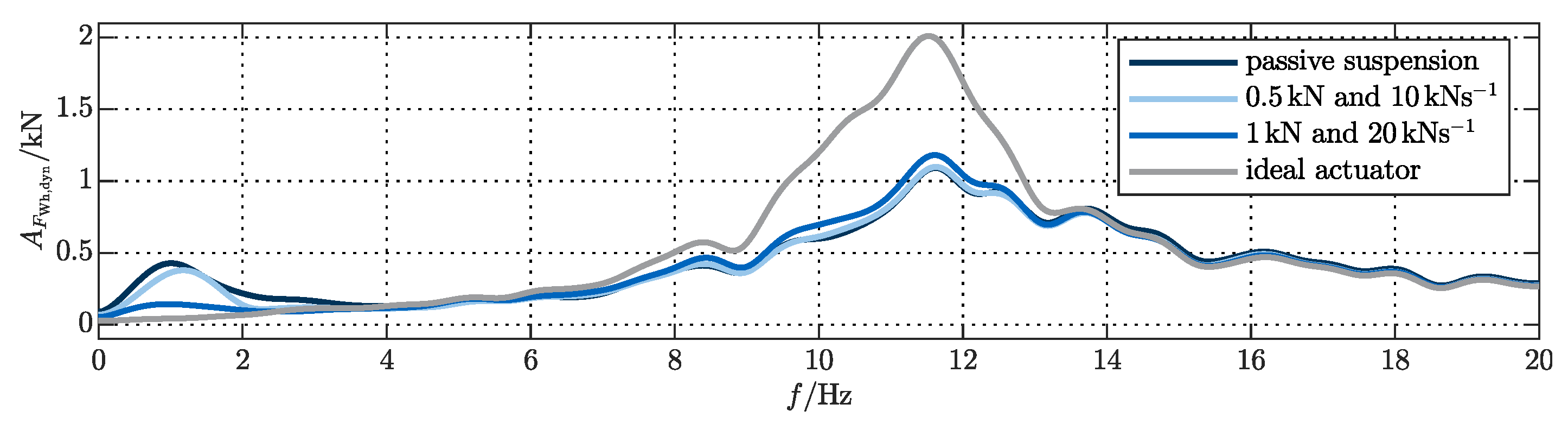
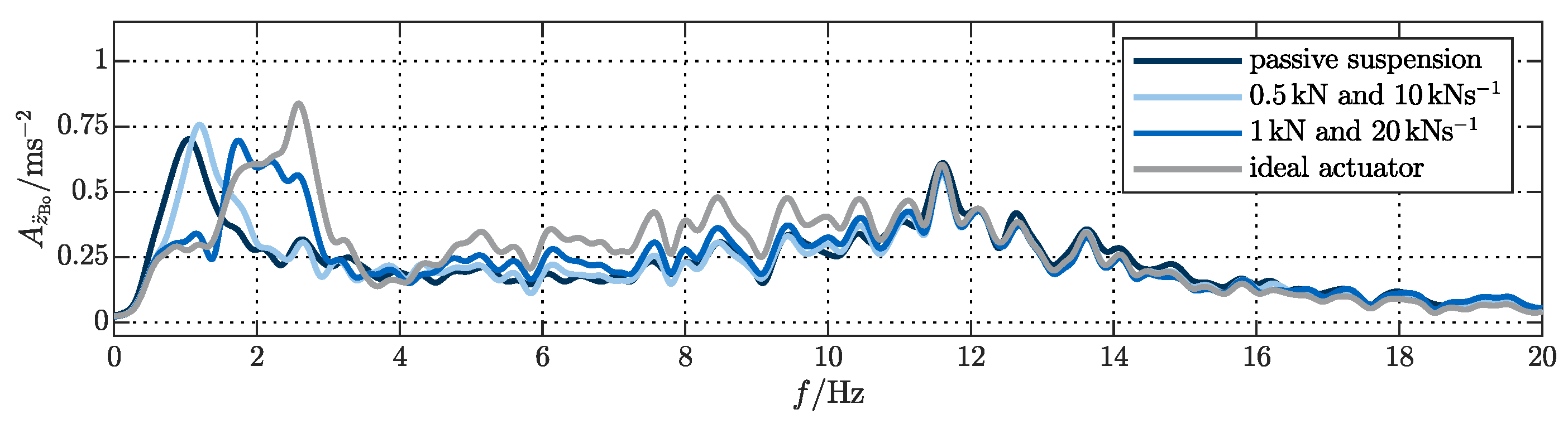
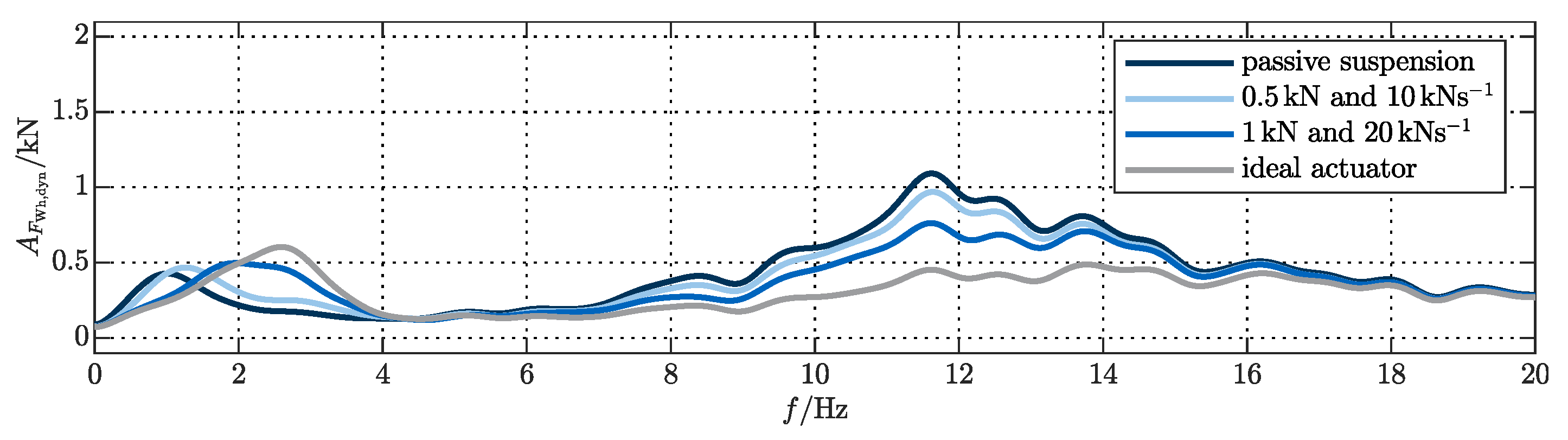
The conflict between ride comfort and road-holding is best described in the frequency domain. Figure 2 shows the frequency response of a quarter-vehicle model in terms of dynamic wheel-load and body acceleration to road excitation for different suspension damping coefficients. The first peak of around 1 Hz corresponds to the body eigenmode, the second peak around 12 Hz to the wheel eigenmode. Low damping results in a high response amplitude of the body acceleration at the body eigenfrequency and low response amplitude between the invariant points [32]. For high damping, the opposite applies. The response of the dynamic wheel-load with low damping is high at the body and the wheel eigenfrequencies. Because humans are sensitive to frequencies between 4 Hz and 10 Hz , it is desirable to have low suspension damping, but this results in high dynamic wheel-load variations, which in turn results in bad road-holding, because the side force potential of the tire decreases with increasing wheel-load variations. Higher damping would be beneficial for good road-holding, but this entails higher body accelerations and less ride comfort. Active systems can resolve this conflict but still have to find a balance between these objectives [33] (p. 267).

2.4. Semi-Active and Active Suspension Control

To resolve the conflict between ride comfort and road-holding, a suitable control algorithm needs to be implemented that outputs the required forces, which in turn need to be supplied by the actuators. Suspension systems can be classified as, passive, slowly-variable/adaptive, semi-active and active systems [34]. In the following, research on control strategies for semi-active and active systems will be summarized, including the application of model predictive control.
The first concept for the vertical dynamics control of active vehicle suspensions was developed by Karnopp [35]. This approach was later extended to semi-active force generators [36]. Ten years after the introduction of the skyhook principle, a modal control concept for fully active suspensions was developed by Wright and Williams [20]. A comparison of SHC and LMC, as well as more information on each controller can be found in [37]. Linear optimal control theory, developed by Anderson [38], was also applied to vertical vehicle dynamics control [39,40,41]. A thorough literature review on the application of LQ-optimal control can be found in [42]. Another important research topic is the use of preview information for suspension control, which is investigated in [43,44,45,46]. Furthermore, model and parameter uncertainties can be incorporated by using H -control [47,48]. An example of adaptive non-linear control is given in [49]. The skyhook control logic is extended to triple-skyhook control in [50], while an alternative to the skyhook principle is acceleration-driven damping, which was developed by Savaresi et al. [51,52]. General summaries of control methods for semi-active suspensions can be found in [53,54] and for active suspensions in [55]. An analytic derivation of performance constraints and limitations in vertical vehicle dynamics control is given in [56].
The latest research in the field focuses on new signal differentiation methods [57], improved vehicle stability control with active suspension systems [58], optimal control application [59,60], preview strategies [61,62,63], incorporating physiological and psychological effects [64], adaptive controllers [65,66,67,68] and fault tolerant control [69]. A multi-objective optimization method for semi-active suspensions is shown in [70]. A non-linear controller considering actuator and state constraints is developed in [71]. Actuator time delays are included in [72,73], while actuator dynamics are introduced in [74,75,76]. Clipped optimal control for vehicle suspensions is presented in [77]. Another way to incorporate system and actuator constrains is model predictive control.
Model predictive control (MPC) can be regarded as an advancement of optimal control. An overview of the history and industrial application of MPC is given in [78]. The first application of MPC to vertical vehicle dynamics control of which the authors are aware is presented in [79,80]. Robust MPC [81] and fast MPC [82,83] were applied later. A comparison of MPC to clipped optimal control is given in [84]. One of the main problems of real-time MPC in vertical vehicle dynamics control is the requirement of optimization convergence within sampling times of 1–10 ms and the required quality of the road-profile preview. A recent implementation of MPC in low-bandwidth suspension systems is presented by Göhrle [85,86]. He also compares the performance of MPC to other control strategies [61,87] and shows different methods of road-profile estimation [62]. For real-time capable implementations explicit MPC is used, as presented in [88,89,90]. Other recent publications are focusing especially on MPC for semi-active suspension [91,92]. Fault estimation for electro-rheological semi-active dampers is present in [93].

2.5. Research Gap

Recapitulating the previous sections, it is clear that a lot of effort has been invested in developing various kinds of control strategies for active and semi-active suspension systems. A number of different suspension actuators exist, and research has been carried out to understand actuator system properties and performance. However, the current state-of-the-art lacks information on the effect of actuator system properties, such as maximum force and maximum rate of change, on achievable ride comfort. This is not trivial to investigate, because the control system performance depends on actuator performance in conjunction with the performance of the control logic. To fill this research gap, the authors present a new method in this article, which makes it possible to quantify the effect of actuator limitations on achievable ride comfort, while assuring best possible control logic performance through the application of MPC. This approach allows to deduct the actuator characteristics required to achieve desired ride comfort targets and displays the sensitivity of ride comfort with respect to these actuator attributes. It shows the pure influence of the actuator properties for the best possible control input. To the best knowledge of the authors, no method and results comparable to this have previously been published in the literature.

3. Method

This section describes the method used to investigate the influence of actuator limitations on achievable ride comfort. Section 3.1 introduces the simulation model, while Section 3.2 describes the different test scenarios and Section 3.3 presents the data processing and analysis procedures. The simulations were performed in MATLAB© using the Model Predictive Control Toolbox. The underlying theory of MPC can be found in [94,95,96]. The simulation can also be built with non-proprietary software such as Octave or Python using the equations given in Section 3.1 and a suitable solver for convex cost functions.
In optimal control, a feedback law based on the system properties and disturbances is derived for an infinite time horizon. In model predictive control, this time horizon is finite and set to a certain preview time referred to as prediction horizon (PH). The control horizon defines the number of preview steps for which an optimal control input is calculated. Whereas in optimal control, a constant feedback matrix is derived for the controller, in MPC the optimization problem is solved in each time step through the PH. At the end of a time step, the optimal control for the next time step is outputted as control demand to the actuator. In the next time step, the system states and PH are updated and the optimization is solved again. This is referred to as receding horizon optimization. As it involves the repeated calculation of an updated feed-forward control problem, MPC is a form of feedback control, because it always starts from measured or estimated states that are independent of model inaccuracies and dependent on non-modelled disturbances. Convergence of the optimization solution within one sampling interval is a prerequisite for real-time implementation of MPC, which is hard to achieve and a reason for research work into explicit MPC. The performance of MPC in a real vehicle is also highly dependent on quality of the preview information, which has to be estimated from sensor measurements of the vehicle (camera, lidar, etc.), or needs to be supplied from a back-end (cloud) for the current position of the vehicle. In this research work here, MPC is used as a tool to obtain the theoretically best solution, considering given actuator limitations. There is no need for real-time feasibility, and preview information as well as system states are known exactly in all the simulations. Detailed information about the structure of the MPC in this research is given in Section 3.1.3.

3.1. System Modelling

This subsection introduces the different parts of the simulation model. First, the vehicle model and the derivation of the discrete-time state-space model is explained in Section 3.1.1, the generation of the stochastic road-profile and the single-obstacle are presented in Section 3.1.2. The synthesis of the MPC controller including the derivation of the cost function, is described in Section 3.1.3. Finally, the implementation of the actuator limitations (input constraints) and boundary conditions (output constraints) is presented in Section 3.1.4, along with the weighting of the optimization objectives.

3.1.1. Vehicle Model

The equations of motion for the quarter-vehicle model in Figure 1 are shown in Equation (1). The model has two degrees of freedom, which results in two equations of motion.
m Bo z ¨ Bo = c Bo z Bo z Wh d Bo z ˙ Bo z ˙ Wh + F Ac
m Wh z ¨ Wh = c Bo z Bo z Wh + d Bo z ˙ Bo z ˙ Wh c Wh z Wh z Ro d Wh z ˙ Wh z ˙ Ro
These can be formulated as a continuous-time state-space model (Equation (2)) with system matrix A c , input matrix B c , transition matrix C c , feedthrough matrix D c , state vector x ( t ) , input vector u ( t ) and output vector y ( t ) .
x ˙ ( t ) = A c x ( t ) + B c u ( t )
y ( t ) = C c x ( t ) + D c u ( t )
Equation (2a) is the state equation and Equation (2b) is the output equation. The matrices and vectors of Equation (2) can be found in Appendix A. This form of the state-space representation with the chosen states was also used in [65]. The model is transformed into a discrete-time state-space model with sample time t s , according to Equation (3).
A d = exp ( A c t s )
B d = A d I 4 A c 1 B c
C d = C c
D d = D c
Another option would be to use the forward Euler method to transform the model. The delay of the actuator force is absorbed into the state-space model by defining a new state vector containing the delayed actuator force, and a new input vector containing the actuator force which is calculated in the current step.
x k * = z Bo , k z Wh , k z ˙ Bo , k z Wh , k z Ro , k z ˙ Ro , k F Ac , k 1 ; u k * = F Ac , k z ˙ Ro , k
The state-space matrices then have to be transformed accordingly. The state matrix is changed so that the current force becomes the delayed force in the next time step, and the input matrix is changed so that only the delayed input is used to calculate the new states.
A = A i j ( d ) 6 p t B i 1 ( d ) 6 p t 0 1 , 4 0 ; B = 0 4 , 1 B i 2 ( d ) 6 p t 1 0 ; C = C i j ( d ) 6 p t D i 1 ( d ) 6 p t ; D = 0 3 , 1 D i 2 ( d ) 6 p t
The discrete state-space model is then given as
x k + 1 = A x k + B u k
y k = C x k + D u k
with the state solution
x k = A k x 0 + i = 0 k 1 A k i 1 B u k
and the output solution
y k = C A k x 0 + i = 0 k 1 A k i 1 B u k + D u k

3.1.2. Road Model

The inverse Discrete Fourier Transform (DFT) method of Cebon and Newland [97] is used to generate a road surface profile, which is subsequently used as disturbance input. It is implemented according to Agostinacchio et al. [98], where the height profile is calculated as:
z Ro ( x ) = i = 0 N Δ n 2 k r · 10 3 n 0 i Δ n cos 2 π i Δ n x + φ i
n max = 1 B Δ n = 1 L N = n max Δ n
In Equation (7), the total length of the road-profile is L (in m ), with a sampling interval of length B (in m ). This defines the maximum spatial sampling frequency resolution ( n max ), which produces N equally spaced spacial frequency domain points in the interval from 0 to Δ n . Using the reference spatial frequency n 0 = 0.1 / m and a set of random and uniformly distributed phase angles φ i in the interval of 0 ; 2 π , a road-profile can be generated in dependency of the parameter k r , which corresponds to an ISO 8608 [99] road roughness classification according to Table 1.
Following generation by inverse DFT, the profile is filtered with a moving average filter of length l cp , which is the assumed contact patch length of the tire. Finally, the profile is converted to a height profile as a function of time, using the vehicle speed as in Equation (8):
z Ro ( t ) = z Ro ( x / v x , veh )
The single-obstacle (bump) is modelled according to Equation (9) as a half-sine wave [30] (pp. 345–346) with height 2 h ^ = 0.1   m and length L = 3.8   m .
f ( x ) : = 0 for x 0 and x L h ^ 1 cos 2 π L x for x 0 and x L

3.1.3. Controller Design

In order to investigate the influence of actuator limitations on achievable ride comfort, it is necessary to exclude to the influence of controller performance. In general, an optimal control problem is formulated, which results in the best possible control input for the actuator. In the case of vertical vehicle dynamics control, it is necessary to incorporate constraints on the dynamic wheel-load and suspension travel (see Section 3.1.4). In optimal control, these constraints can only be considered indirectly via the cost function, and the optimization problem needs to be solved over the whole length of the simulation. MPC allows explicit consideration of these constraints and divides the problem into sub-problems of the size of the prediction horizon, which results in faster computation time, and was therefore used in this investigation.
Figure 3 shows a schematic overview of the simulation model with the MPC controller. The vehicle plant model from Section 3.1.1 is also used in the MPC controller. At time step k, the road disturbance v k is inputted to the plant, and the vector of road disturbances over the preview horizon v ˜ k is inputted to the MPC controller. The current state vector x k of the plant is also inputted to the MPC controller. This controller computes the optimal sequence of control inputs over the prediction horizon u ˜ k with respect to the cost function (Equation (17)), which is depending on the vector of outputvectors y ˜ k over the prediction horizon (PH). The first input of the computed optimal control sequence is then inputted to the plant for the next time step. To derive the cost function, it is necessary to split the input into actuator input u and road disturbance v, as shown in Equation (10).
x k + 1 = A x k + b ( u ) u k + b ( v ) v k
y k = C x k + d v k
b ( u ) = B i 1 ; b ( v ) = B i 2 ; d = D i 2 ; u k = F Ac , k ; v k = z ˙ Ro , k
The state solution becomes
x k = A k x 0 + i = 0 k 1 A k i 1 b ( u ) u k + b ( v ) v k
and the output solution
y k = C A k x 0 + i = 0 k 1 A k i 1 b ( u ) u k + b ( v ) v k + d v k
The solutions for the next p steps over the PH can be written in matrix form as
y k + 1 y k + 2 y k + p = CA C A 2 C A p x k + C b ( u ) 0 0 CA b ( u ) C b ( u ) 0 C A p 1 b ( u ) C A p 2 b ( u ) C b ( u ) u k u k + 1 u k + p 1 + + C b ( v ) d 0 0 CA b ( v ) C b ( v ) d 0 C A p 1 b ( v ) C A p 2 b ( v ) C A p 3 b ( v ) d v k v k + 1 v k + p
and by defining
y ˜ = y k + 1 y k + 2 y k + p ; u ˜ = u k u k + 1 u k + p 1 ; v ˜ = v k v k + 1 v k + p ; Ω = CA C A 2 C A p ;
Γ u = C b ( u ) 0 0 CA b ( u ) C b ( u ) 0 C A p 1 b ( u ) C A p 2 b ( u ) C b ( u ) ; Γ v = C b ( v ) d 0 0 C A b ( v ) C b ( v ) d 0 C A p 1 b ( v ) C A p 2 b ( v ) C A p 3 b ( v ) d ;
Equation (13) becomes
y ˜ k = Ω x k + Γ u u ˜ k + Γ v v ˜ k
Using Equation (14) and introducing the weighting matrix W , which is used for each time step and gives a vector of matrices W ˜ , the vector of slack variables ϵ and the constraint violation penalty ρ , the cost function for the optimal control problem over the prediction horizon can defined as:
J k u ˜ k , ϵ = Ω x k + Γ u u ˜ k + Γ v v ˜ k T W ˜ Ω x k + Γ u u ˜ k + Γ v v ˜ k + ϵ T ρ ϵ
and rewritten as
J k u ˜ k , ϵ = 1 2 u ˜ k T Γ u T W ˜ Γ u u ˜ k + x k T Ω ˜ T W ˜ Γ u + v ˜ k T Γ v T W ˜ Γ u u ˜ k + 1 2 ϵ T ρ ϵ +            + 1 2 v ˜ k T Γ v T W ˜ Γ v v ˜ k + x k T Ω T T ˜ 2 Γ v v ˜ k + x k T Ω T W ˜ Ω x k
The cost function is only a function of the input and the slack variable, and all terms that do not include these are constant and can be ignored. The final cost function is shown in Equation (17).
J k u ˜ k , ϵ = 1 2 u ˜ k T Γ u T W ˜ Γ u u ˜ k + x k T Ω ˜ T W ˜ Γ u + v ˜ k T Γ v T W ˜ Γ u u ˜ k + 1 2 ϵ T ρ ϵ
The QP KWIK solver [100], which is based on the dual algorithm of Goldfarb and Idnani [101], is used to solve the quadratic problem in order to obtain the optimal control inputs for each time step. This algorithm is pre-implemented in the MATLAB© Model Predictive Control Toolbox, but can also be implemented in non-proprietary software such as GNU Octave or other programming languages. Another option is to use a solver from the YALMIP toolset [102] if the Model Predictive Control Toolbox and Optimization Toolbox are not available in MATLAB©.

3.1.4. Actuator Limitations, System Constraints and Weights

The optimization problem formulated in Equation (17) needs to be solved with consideration for the constraints of the control input (actuator force and rate) and output constraints on the dynamic wheel-load and suspension travel. This is necessary to ensure that the problem solution stays within the valid range of the simulation model. The optimization problem is therefore subject to the following linear inequality input constraints
F Ac , min F Ac , k F Ac , max
F ˙ Ac , min F ˙ Ac , k F ˙ Ac , max
and output constraints
F dyn , min ϵ k F dyn , k F dyn , max + ϵ k
z sus , min ϵ k z sus , k z sus , max + ϵ k
F Ac , k is the actuator force (control input) at time step k , F dyn , k and z sus , k are the discrete output values of the dynamic wheel-load and the suspension-deflection. The full output vector including the body acceleration a Bo , k is shown in Appendix A. The values of the constraints on the actuator force are shown in Section 3.2. For all simulations, the output constraints were set according to Table 2.
The constraint on the dynamic wheel-load ensures that the actual wheel-load (static + dynamic) is always positive and lift off does not occur. Lift off is non-linear and can therefore not be incorporated in this model. The maximum value of the dynamic wheel load in pressure is unconstrained. The suspension travel is limited to 10   c m to ensure that it stays within the linear range. This value is set conservatively and may be increased depending on the vehicle. Unlike the input constrains, the output constraints are soft constraints, which allows for a minor violation of the constraint. It is done to ensure feasibility of the optimization problem. The validity of the results was checked in post-processing, see Section 3.3.
Figure 4 shows an example of the implementation of the actuator constraints in the controller. The dashed red line shows the desired force of a non-restricted controller without delay. The blue line shows the force of a controller, in which the maximum force is limited to 2000   N and the maximum rate to 10   k N   s −1. The restricted force also contains the delay of one time step from controller output to actuator input. The dotted orange line shows the highest possible change of the actuator force according to the rate constraint. At around 0.04   s , the unrestricted force changes with a step to 2500   N . The restricted force starts to rise accordingly at the maximum rate of change, delayed by one time step, and saturates at the maximum force limit. At around 0.45   s , the desired force descends below the maximum force limit at a rate smaller than the maximum rate restriction. The restricted force follows the unrestricted, delayed by one time step. Finally, the unrestricted force drops from 1000   N to 0   N , and the restricted force follows in compliance with the rate limitation.

3.2. Test Scenarios

Different test scenarios were used in this research, defined by the road-profile, the vehicle speed and the optimization objective (Table 3). A simulation was performed on the single-obstacle profile at 36   k m   h −1, with the objective of minimizing the vehicle body acceleration for comfort. The single-obstacle profile is shown in Figure 5. The figure only shows the section of the bump; the full profile is extended as a flat road before and after the bump.
On the stochastic road-profile A-B, three simulations were carried out at speeds of 45   k m   h −1, 90   k m   h −1 and 180   k m   h −1. In all three cases, the objective was to minimize the vehicle body acceleration. On the B-C profile, two simulations were performed at 90   k m   h −1; in one case, the objective was to minimize the body acceleration, while in the other case, the objective was to minimize the dynamic wheel-load variation. Figure 6a shows the stochastic road-profiles. The spatial power spectral density of the stochastic road-profiles can be seen in Figure 6b.
All simulations were carried out at a sampling frequency of 100   Hz and a preview horizon of 2   s . The control horizon was set to its maximum of 1.99   s , which is one sample less than the preview horizon. A summary of these settings is given in Table 4. The quarter-car model is parameterized according to Table 5. These parameters correspond to a vehicle with a total mass of 2200   k g , a body eigenfrequency of 1.1   Hz , a wheel eigenfrequency of 12.2   Hz and 22 % critical damping. These are exemplary values for a modern, premium class luxury vehicle, for example a BMW 7-Series or a Mercedes S-Class. The formulae for calculating the full vehicle parameters can be found in Appendix B.
The actuator limitations of maximum force and maximum rate of change were varied from 0   N to 10,000 N and 0   N   s −1 to 10,000 N s1 respectively. A passive vehicle and a vehicle with an MPC controller without input constraints were also simulated according to the scenario. The passive vehicle was the baseline and the ideal MPC vehicle was the reference for what could be achieved in the best case. Table 6 shows the different values of the input constraints in the single-obstacle scenario. They were defined in an iterative process to achieve good resolution in the areas of interest; these are shown in Section 3.3. All combinations of force and rate constraints were simulated.
Table 7 shows the different input constraints for the stochastic road-profile scenarios. All possible combinations were simulated. Compared with the limitations for the bump-profile, the values were chosen to have better resolution at lower maximum force limits and higher maximum rate of change limits. Again, this was determined in preliminary experiments and will be explained in Section 3.3.
Table 8 shows the weighting factors, which were used for the two different optimization objectives. Each one consists of the relative weighting factor in bold font and a normalization term in brackets. Normalization is used to even out the order of the different variables, which is necessary to apply relative weighting. The weighting factor for the slack variable ( ρ ) was always set to 1 × 10 10 . For optimizing minimum body acceleration, the relative weighting for body acceleration w z ¨ Bo was set to 10, while relative weighting factors for suspension-deflection w z sus and dynamic wheel-load w F dyn were set to 0.1 . These three weighting factors form the trace of the diagonal weighting matrix W , which is concatenated to the vector of weighting matrices W ˜ in the cost function (Equation (17)). Suspension-deflection and dynamic wheel-load weighting were set to non-zero, because otherwise the controller would not consider these in the optimization, and run into the respective constraint, resulting in poorer minimization of body acceleration. For optimization with respect to the dynamic wheel-load, the weighting factor w z sus was increased to 1, because the controller was more prone to hitting the suspension-deflection constraint. An additional term to consider the actuator force was also added to the cost function for stability reasons. Without this term, the controller would become unstable with this objective. It was added by defining another output equation for the input force and adding the weighting factor w F act to the weighting Matrix W . It avoids the input force increasing beyond all limits and become unstable. The value was determined by performing a sensitivity analysis with respect to the minimal achievable dynamic wheel-load variation.

3.3. Data Processing and Analysis

A number of steps were carried out to obtain the results presented in this research paper. The process is summarized in Figure 7. As shown in Section 3.2, each scenario was simulated with a variety of actuator constraints and therefore consists of multiple simulations. A single simulation outputs the trajectories of the body acceleration z ¨ Bo , suspension travel s sus and dynamic wheel-load F dyn , along with information about the MPC solution in each time step. This information contains the slack variable, the number of iterations of the solver, the computation time and whether an optimal solution could be obtained.

3.3.1. Evaluation of the Single Simulation Results

In this investigation, the root mean square (RMS) value is used to quantify the outputs of a simulation ( z ¨ Bo , s sus and F dyn ). The ISO 2631 cannot be used here, for two reasons. First, the model only outputs the vertical body acceleration, so, the directional weighting of the ISO 2631 cannot be applied and the comfort value would not show a benefit compared to an analyses of the RMS value. Second, the frequency weighting of the ISO 2631 is a non-linear operation and therefore cannot be directly implemented in the MPC controller. In the case of the quarter-car model, the reduction of the body acceleration directly correlates to the reduction of the ISO 2631 comfort value, as can be seen in Figure A1 in Appendix C. The plausibility and validity of the results were also checked, as were violated constraints and reasonable trajectories of the state and output variables. Minor violations of the dynamic wheel-load and suspension travel limits were considered admissible because the suspension travel limit was set conservatively to ± 5 c m . In reality, the wheel could lift off for a short time and the inertia of the wheel could be used to generate a force larger than the static wheel-load. The maximum and mean values of the violations are shown in Appendix E, along with the number of violation time steps.

3.3.2. Processing of the Scenario Data

In order to enable a condensed overview of the results in each scenario, the results of the single simulations are subjected to further processing. First, the RMS results are combined into a surface as a function of the maximum force and the maximum rate constraint. This surface is displayed as surface plots for z ¨ Bo , s sus and F dyn and as contour plots for z ¨ Bo or F dyn respectively. Additionally, the gradient of the surface of z ¨ Bo or F dyn is calculated and used to display the trajectory of gradient-descent from the origin. This trajectory line can be used to analyze the optimal combination of force and rate limitations. In other words, it makes it possible to see how much rate of change an actuator should be able to supply for a given target of maximum force, and vice versa.

4. Results

The following section presents and describes the results for the different simulation scenarios. These include RMS surface plots of the body acceleration z ¨ Bo , the dynamic wheel-load F dyn , the suspension-deflection s sus and the actuator force F act , as well as a contour plot of the body acceleration z ¨ Bo or dynamic wheel-load F dyn with the gradient-descent line. FFT gain plots of the body acceleration z ¨ Bo and the dynamic wheel-load F dyn are given in Appendix D and Appendix E along with heat-map plots showing possible constraint violations. The results of each scenario in the passive simulation and the unrestricted MPC actuator simulation are summarized in Table 9.
In the single-obstacle bump scenario, the MPC controller can reduce body acceleration from 1.29   m s 2 to 0.05   m s 2 and dynamic wheel-load variation from 611   N to 211   N . Although the objective was to minimize body acceleration, in the case of the single-obstacle with a smooth surface, the reduction of body acceleration also entailed a reduction in dynamic wheel-load variation, because the bump mainly excited the body eigenmode. Suspension-deflection RMS was slightly reduced from 2.2   c m to 2.0   c m , and the RMS actuator force was 528   N . On the AB profile at 90   km h 1 , the body acceleration RMS was reduced from 0.71   m s 2 to 0.01   m s 2 , at the cost of an increase in dynamic wheel-load variation from 987   N to 1840   N . Suspension travel is also slightly increased from 0.7   c m to 1.0   c m and the RMS actuator force was 580   N . At 45   km h 1 on this profile, the body acceleration was reduced from 0.38   m s 2 to 0.004   m s 2 , with an increase from 503   N to 1160   N in dynamic wheel-load variation. Suspension travel is increased from 0.4   c m to 0.6   c m with an RMS actuator force of 362   N . At 180   km h 1 , the body acceleration decreased from 1.54   m s 2 to 0.48   m s 2 . Due to the constraints on dynamic wheel-load and suspension-deflection, the MPC controller was not able to decrease the body acceleration any further. The dynamic wheel-load variation rose from 1960   N to 2626   N , suspension-deflection RMS showed a small increase from 1.8   c m to 1.9   c m , and the actuator RMS force was 846   N . On the BC profile where the objective was to minimize body acceleration, it was reduced from 1.51   m s 2 to 0.54   m s 2 . Again, the controller was not able to reduce the body acceleration RMS any further due to the output constraints. Dynamic wheel-load and suspension-deflection increased from 2024   N to 2762   N and from 1.6   c m to 1.9   c m respectively. The RMS actuator force was 884   N . When the objective was to minimize dynamic wheel-load variation, its RMS value was decreased to 1412   N at the cost of an increase in body acceleration RMS to 1.81   m s 2 . Here, the suspension-deflection RMS value fell to 0.5   c m and the actuator RMS force was 737   N .

4.1. Single-Obstacle Bump

In the single-obstacle scenario, the vehicle drove over a bump (see Section 3.2) at a speed of 36   km h 1 . This resembles a situation in a restricted traffic zone in a residential area. Figure 8 shows the RMS surface plots for this scenario. In each plot, the lower left axis denotes the maximum actuator force F Ac , max in k N , and the lower right axis represents the maximum actuator rate of change F ˙ Ac , max in kN s 1 . The z-axis shows the respective RMS values. In each plot, the intersection of the surface with the xz and xy plane corresponds to the RMS value of the passive vehicle. The transparent grey plane shows the result for the MPC controller with a non-restricted actuator. In this scenario, the reduction in body acceleration also led to a reduction in dynamic wheel-load variation, because the bump mainly excited the vehicle’s body eigenmode. Both decrease with increasing maximum force and rate limit. The suspension-deflection RMS decreases for low maximum forces, and peaks for low maximum force and high rate of change limits. The RMS actuator force saturates around a maximum force limit of 1.5   k N and a maximum rate limit of 10   kN s 1 .
Figure 9 shows the contour plot of the RMS body acceleration with isolines from 0.9   m s 2 to 0.05   m s 2 in 0.2   m s 2 steps. The closer the isolines are to each other, the steeper the gradient of the surface in this area. It can be seen that the RMS body acceleration depends greatly on the maximum rate limit and that a relatively small maximum force is sufficient, provided the actuator can supply a high enough rate of change. The largest decrease in body acceleration can be seen up to a maximum force limit of 1500   N , and no further decrease in body acceleration can be achieved with maximum forces larger than 2250   N . This can be deduced by following the gradient descent line, which points completely in the direction of the increased rate of change limit, after 2250   N at 26   kN s 1 . The perpendicular shape of the isolines also shows that it is not possible to compensate a low maximum rate of change with a high maximum force limit and vice versa. For a target value of 0.1   m s 2 the ideal actuator (minimum maximum force and maximum rate) for the chosen output constraints would have a maximum force of around 2000   N and a maximum rate of change of around 21.5   kN s 1 .
The FFT plots of body acceleration (Figure A2) and dynamic wheel-load (Figure A3), which display the amplitude of the signals in the frequency domain for different actuator configurations, can be found in Appendix D. Here, it can be seen that the vehicle is mainly excited in the body eigenfrequency range and that the controller lowers the peak for increasing actuator potential. No violation of the dynamic wheel-load constraint occurred in this scenario. Suspension-deflection constraint violations larger than 0.5   m m only occurred in the simulations with a maximum force limit of 250   N and 500   N , with rate constraints of up to 3   kN s 1 .

4.2. Road-Profile AB

Three different scenarios were investigated on the AB road-profile (see Section 3.2). The objective was to minimize body acceleration while travelling at 90   km h 1 , 45   km h 1 and 180   km h 1 . The 90   km h 1 scenario corresponds to travelling on a good country road, the 45   km h 1 scenario to inner city driving and the 180   km h 1 scenario to driving on a German motorway.

4.2.1. Good Country Road at 90   km h 1

In the first scenario with a speed of 90   km h 1 , the body acceleration RMS was reduced to nearly zero at the cost of an almost doubled dynamic wheel-load variation, as shown in Figure 10. Suspension travel RMS shows a moderate increase with a maximum for low maximum rate limits and high maximum force limits. Suspension-deflection is smallest for maximum force limits smaller than 1000   N . Actuator force RMS increases with increasing maximum force and rate limits up to the value of the unrestricted actuator.
Figure 11 shows the contour plot of the body acceleration RMS values, with isolines from 0.5   m s 2 to 0.1   m s 2 in 0.1   m s 2 steps. Again, the influence of the actuator rate of change is dominant, and the perpendicular contour lines indicate that an increase in one limit cannot compensate for the restriction due to the other one. The gradient is steepest for actuator maximum force limits smaller than 1000   N . Above this limit, the actuator rate of change is predominant. For a target value of 0.1   m s 2 RMS body acceleration, the ideal actuator for the chosen output constraints would need to have a maximum force of roughly 1400   N and a maximum rate of change of about 62   kN s 1 in this scenario. Above a maximum force limit of 2000   N and a maximum rate limit of 100   kN s 1 , no significant decrease in body acceleration RMS value could be achieved.
The FFT plots of body acceleration (Figure A4) and dynamic wheel-load for selected limits can be found in Appendix D. They show how a decrease in body acceleration leads to an increase in dynamic wheel-load variation around the wheel eigenfrequency. Even though the MPC controller reduces the dynamic wheel-load variation at the body eigenmode and can hold the variation at the level of the passive suspension between 3   Hz and 8   Hz and above 14   Hz , it cannot avoid the increase around the wheel eigenfrequency, where the objective is to minimize body acceleration.
Contrary to the single-obstacle scenario, there was no violation of the suspension-deflection limit. Instead, for maximum force limits higher than 1000   N combined with rate limits above 70   kN s 1 , a small violation of the dynamic wheel-load constraint appeared (Appendix E, Figure A15). The worst case is a violation in three time steps with a mean value of 589   N , which is around 10 % of the static wheel-load for 0.03   s .

4.2.2. Inner City at 45   km h 1

The RMS performance indicators in Figure 12 show qualitatively the same characteristics in the inner city scenario as for the good country road scenario, but at a quantitatively lower level. The body acceleration RMS value saturates early at the level of the unrestricted actuator. This is also the case for suspension-deflection, dynamic wheel-load and actuator force RMS values.
Qualitatively, the contour plot of the body acceleration in this scenario is also comparable to the good country road scenario, as shown in Figure 13. However, the gradient descent line is shifted slightly downwards, and for a target value of 0.1   m s 2 , the ideal actuator would only need to supply a maximum force of around 600   N and a maximum rate of around 24   kN s 1 under the chosen output constraints. Above a 1600   N maximum force limit and 82   kN s 1 , no further improvement in body acceleration RMS can be observed. The FFT plots of this scenario are shown in Appendix D, Figure A6 and Figure A7. No constraints were violated in this scenario.

4.2.3. Motorway at 180   km h 1

The final scenario on the AB profile is driving on the motorway at 180   km h 1 . Again, qualitatively, the RMS surface plots in Figure 14 show the same behavior as in the 45   km h 1 and 90   km h 1 scenarios, but this time shifted to higher values. Furthermore, the RMS values only approach the values of the unrestricted actuator for the highest maximum rate limitations and maximum force limits above 1500   N , and the body acceleration RMS value can only be reduced to 0.48   m s 1 .
In the contour plot in Figure 15, the gradient descent line is shifted upwards compared to the other two scenarios with the AB profile. However, as with the other scenarios, one limit cannot compensate for the other one. In this case, the target value of 0.1   m s 1 cannot be reached. Instead, 0.6   m s 1 is used as a target, both here and for the BC profile. To achieve this RMS body acceleration, the ideal actuator would need to have a maximum force of 1600   N and a maximum rate of 52.5   kN s 1 .
The FFT plots in Appendix D show that an actuator with a 1000   N maximum force and a maximum rate of 52.5   kN s 1 can significantly lower the body acceleration and dynamic wheel-load variation up to 3   Hz , while maintaining the wheel-load variation of the passive suspensions at 3   Hz and above. A further decrease in body acceleration, achieved with the unrestricted actuator, entails much higher dynamic wheel-load variation around the wheel eigenfrequency. In this scenario, the dynamic wheel-load constraint was the restrictive one. In Figure A16 in Appendix E, it can be seen that the most violations occurred in the simulations where the maximum force was higher than 1000   N and the rate limits were above 50   kN s 1 . However, their maximum and mean value is only 5   N , which is negligible. The only relevant violations with mean values between 200   N and 300   N occurred in the simulation with the lowest rate or lowest force constraint. These only occurred in two to three time steps, which is admissible.

4.3. Road-Profile BC

Two scenarios were carried out on road-profile BC, which were both driven at 90   km h 1 . This corresponds to travelling on a substandard country road in Germany. In one scenario, the objective was again to minimize body acceleration, while in the other, it was to minimize the dynamic wheel-load variation.

4.3.1. Bad Country Road at 90   km h 1

The RMS values in this scenario are comparable to the RMS values of the scenario on the AB profile at 180   km h 1 , as can be seen in in Figure 16. The only difference is that the body acceleration cannot be minimized so well for low maximum force and rate limitations, and the lowest possible body acceleration RMS value is slightly higher.
In the contour plot of RMS body acceleration in Figure 17, it can be seen that the gradient for the maximum force is steepest up to 1000   N . Here too, the rate limitation has the biggest influence on the reduction in body acceleration. No relevant further improvement can be seen for maximum force values above 2600   N . To achieve the target value of 0.6   m s 2 , the ideal actuator would need to posses a maximum force of 2000   N and a maximum rate of 67   kN s 1 under the chosen output constraints. >From the FFT plots of body acceleration (Figure A10) and dynamic wheel-load (Figure A11) in Appendix D, it ca be seen that an actuator with a maximum force of 500   N and a maximum rate of 10   kN s 1 is hardly able to reduce the body eigenfrequency peak compared to the passive vehicle, and it is this that constitutes the main difference to the 180   km h 1 AB profile scenario. It is thus the main reason why actuators with low maximum force and rate limits have higher body acceleration RMS values on the BC profile. In terms of dynamic wheel-load constraint violations, this scenario is also similar to the 180   km h 1 AB profile scenario, which means there are some minor violations for high force and rate limits and a few larger violations for low maximum force and rate limits, as can be seen in Figure A17. But unlike the other scenario, some violations of the suspension travel limits occurred here too (see Figure A18). This violation was the largest in the simulation with a maximum force of 300   N and a maximum rate of 5   kN s 1 , with a maximum value of 1.2   cm and a mean value of 0.5   cm over 0.19   s , which is still acceptable. In general, the most suspension-deflection violations arose in the simulations with this maximum force or rate limit.

4.3.2. Minimization of Dynamic Wheel-Load on a Bad Country Road

This scenario investigates the requirements placed on the actuator with the objective of minimizing dynamic wheel-load variation. For this investigation, it was necessary to change the weighting factors in the cost function (see Table 8 in Section 3.2). The RMS plots in Figure 18 show that reduction in dynamic wheel-load goes hand in hand with an increase in body acceleration, which is the exact opposite compared to minimizing the body acceleration and clearly indicates that the conflict of objectives, as described in Section 2.3, also exists for active systems. Compared to minimizing body acceleration, the suspension-deflection is also reduced in this case, influenced by the weighting factor for suspension-deflection, which was increased for stability reasons. The actuator force RMS value is lower compared to the other scenario, which is influenced by the addition of the actuator force weighting.
Figure 19 shows the RMS contour plot of the dynamic wheel-load variation. This result indicates that reduction in RMS dynamic wheel-load variation to 1520   N , which already represents 82 % of the possible reduction with an unrestricted actuator, is possible with a maximum force of about 750   N , provided the maximum rate limit is higher than 42   kN s 1 . The ideal actuator for achieving an RMS value of 1420   N under the given constraints would need to have a maximum force of 2250   N and a maximum rate of 72   kN s 1 . No noteworthy improvement in dynamic wheel-load variation is seen for maximum force limits higher than 3000   N and rate limits higher than 100   kN s 1 . Any limits higher than 2250   N and 72   kN s 1 can only reduce the dynamic wheel-load RMS value by a further 8   N at best.
The FFT plots of body acceleration (Figure A12) and dynamic wheel-load (Figure A13) in Appendix D show how the reduction in dynamic wheel-load around the wheel eigenfrequency leads to an increase in body acceleration between 4   Hz and 11   Hz . It can also be observed, that the body eigenfrequency peak is shifted towards 2.5   Hz and that the dynamic wheel-load variation actually worsens between 0   Hz and 4   Hz . The dynamic wheel-load (Figure A19) and suspension-deflection (Figure A20) constraint violations are comparable to those when optimizing for body acceleration. Dynamic wheel-load constraint violation was present in simulations with low maximum force or rate limitations. Suspension-deflection violation was worse again for simulations with a maximum force limit of 300   N or a maximum rate limit of 5   kN s 1 . Contrary to optimization for body acceleration, dynamic wheel-load constraint violations become smaller and disappear for high maximum force and rate limitations, due to the optimization target. Furthermore, the violations of the suspension-deflection constraint are slightly reduced for higher limits, due to the change in its weighting factor.

5. Discussion

The results of this research are discussed in Section 5.1. Points of criticism and potential for future work are outlined in Section 5.2.

5.1. Interpretation of the Results

In general, the results obtained in this research are plausible and were also found to be robust in repeated simulations. If a scenario was repeated multiple times with the same weighting factors and constraints, the results of the individual simulations did not change, which indicates that the optimal trajectory of control inputs for each simulation was unique. Of course the results depend on the chosen weighting factors and constraints. Here, the weighting factors were chose for either maximum comfort or maximum road-holding, so the results would of course change with different objectives. The other influential factors are the output constraints. They were set to maintain a positive wheel-load and to keep the suspension travel within 10   c m . These could also be changed to allow more suspension travel, where possible on the simulated vehicle, or to keep the minimum wheel-load above 0   N , which again would change the obtained results. The purpose of this research article is to present a tool set and method for investigating these dependencies, and as with any simulation tool, it is the responsibility of the user to define reasonable boundary conditions and understand the validity and limitations of the results.
Another point worthy of discussion are the results obtained for low maximum force and maximum rate limits in the bump scenario, the 180   km h 1 AB profile scenario, and the two scenarios on the BC profile. In these simulations, the controller had problems staying within the output constraints on dynamic wheel-load and/or suspension-deflection. This is not a problem of the controller itself, because when the higher limits on the actuator where higher, the controller remained within these constraints. The problem is that not even the passive vehicle stays within the chosen constraints, as can be seen in in Appendix F Table A1. The controller has to balance the objective conflict of trying to stay within the constraints while minimizing body acceleration or dynamic wheel-load. The absolute values in these simulations are very dependent on the output constraint settings. This only occurred for the lowest rate and force limitations on the actuator and does not affect the general results in these scenarios.
Although the focus of this research is on the tool set and the method for investigating the influence of actuator limitations, the results can also be interpreted for the chosen output constraints and weighting factors. In general it could be seen that a relatively low maximum actuator force of around 1000 to 2000   N is sufficient, provided the actuator can supply a high enough rate of change. In most scenarios, a threshold for the maximum force was apparent, after which it was only possible to improve the result with higher rate limits. Table A2 in Appendix F gives an overview of the maximum actuator force and rate limits obtained by choosing arbitrary target values for the body acceleration and dynamic wheel-load RMS. Again, the target value needs to be determined by the user of this method. For the chosen target values of 0.1   m s 2 , 0.6   m s 2 and 1520   N , the actuator needs to supply a maximum force within 600   N to 2250   N and a maximum rate within 21.5   kN s 1 to 72.0   kN s 1 , where the higher force and rate requirements are due to optimization of dynamic wheel-load variation on the BC profile, and the lowest stem from the inner city and single-obstacle scenarios. An actuator with a maximum force of 2000   N and a maximum rate of 60   kN s 1 would therefore be a suitable compromise for these scenarios. Comparing this to the eABC system recently introduced by Daimler [19], which has maximum force limits of 6000   N and 7000   N , and maximum rate limits of 24   kN s 1 and 20   kN s 1 for the front and rear axles of a Mercedes GLE, it can be seen that in terms of ride comfort due to road irregularities, it might have been beneficial to design a system with a lower maximum force and higher rate of change capabilities. However, for requirements on roll and pitch compensation under lateral and longitudinal acceleration, high static forces need to be supplied and the actuator dynamics are of less importance, but with regard to autonomous driving, where vehicles are expected to travel with lower longitudinal and lateral accelerations, the focus might need to shift towards systems with higher rate capabilities and lower maximum forces.

5.2. Critisism and Future Work

This research is the first to present a method for the investigation of actuator limitation influences on ride comfort. There are some things to keep in mind when applying this method. First, it is a simplification to assume that an actuator is perfectly characterized by its maximum force and a constant maximum rate limit. Usually, actuators in suspension control systems show PT-1 or PT-2 behavior as a step response, because the actuator itself has a controller that regulates the output force and is tuned to display stable behavior. This means that the actual rate limitation is a function of the desired step height and the actuator force output is also subject to inaccuracies. Neither are currently considered, but the method can be used to analyze the general sensitivity to these constraints. Another thing to keep in mind is that if the vertical vehicle dynamics controller is of the standard feedback type, such as a sky-hook controller, the actuator rate also influences its stability. The rate of change is even more important, because it is the main reason for the phase delay from the desired to the actual force, and the greater the phase delay, the lower the possible gain of the controller. The aim is to extend this method in the future, so as to encompass actuator accuracy, power limitation, and dynamic actuator behavior using a full vehicle model; this also including roll and pitch dynamics, and the possibility of an active anti-roll bar control system. It is also planned to extend the method to analyze semi-active suspension systems and to compare these results with those from active suspension systems.

Author Contributions

The first author E.E. and the other authors G.B. and N.M. have contributed as follows: “Conceptualization, E.E. and N.M.; methodology, E.E.; software, E.E.; validation, E.E.; formal analysis, E.E.; investigation, E.E.; resources, N.M.; data curation, E.E.; original draft, E.E.; review and editing, G.B.; visualization, E.E.; project administration, E.E. and G.B.; funding acquisition, N.M.” All authors have read and agreed to the published version of the manuscript.

Funding

This research was funded by Bayerische Motorenwerke AG.

Acknowledgments

The authors wish to thank BMW for funding this research project, especially Thomas Kiesewetter, head of department EF-31 and Dirk Frohmüller, group leader EF-311. The authors are also grateful for the valuable contribution of the TUM students Henning Bohlen, Florian Reister, Florian Hartmann and Andreas Kühne, who assisted and continue to assist in the development of the presented method. The authors also wish to express their sincere thanks to Matthias Förth and Alexander Wischnewski of TUM for their constructive exchange of views on model predictive control and optimization problems.

Conflicts of Interest

The authors declare no conflict of interest. The funders had no role in the design of the study, in the collection, analyses, or interpretation of data, in the writing of the manuscript, or in the decision to publish the results.

Abbreviations

The following abbreviations are used in this manuscript:
ARBAnti-Roll Bar
BMWBayerische Motoren Werke
BSBritish Standard
CHControl Horizon
CVDContinuously Variable Dampers
DFTDiscrete Fourier Transform
eABCElectronic Active Body Control
EVElectric Vehicle
FFTFast Fourier Transform
ICEInternal Combustion Engine
ISOInternational Organization for Standardization
LMCLotus Modal Control
LQGLinear-Quadratic Gaussian Regulator
LQRLinear-Quadratic Regulator
MPCModel Predictive Control
PHPrediction Horizon
RMSRoot Mean Square
SHCSky-Hook Control
TUMTechnical University of Munich
VDISociety of German Engineers

Appendix A

A c = 0 1 0 1 c Bo / m Bo d Bo / m Bo 0 d Bo / m Bo 0 0 0 1 c Bo / m Wh d Bo / m Wh c Wh / m Wh d Bo + d Wh / m Wh ; B c = 0 0 1 / m Bo 0 0 1 1 / m Wh d Wh / m Wh ;
C c = c Bo / m Bo d Bo / m Bo 0 d Bo / m Bo 0 0 c Wh d Wh 1 0 0 0 ; D c = 1 / m Bo 0 0 d Wh 0 0 ;
x ( t ) = z Bo ( t ) z Wh ( t ) z ˙ Bo ( t ) z Wh ( t ) z Ro ( t ) z ˙ Ro ( t ) ; y ( t ) = z ¨ Bo ( t ) F dyn ( t ) s sus ( t ) ; u ( t ) = F Ac ( t t s ) z ˙ Ro ( t )

Appendix B

Formulae for calculating the full vehicle parameters:
m Veh = 4 m Bo + m Wh
f Bo = 1 2 π c Bo m Bo
f Wh = 1 2 π c Bo + c Wh m Wh
D Bo = 100 · d Bo 2 c Bo m Bo

Appendix C

Figure A1. Comparison of RMS body acceleration and ISO-2631 comfort value (weighted RMS) at 90   k m   h −1 on the AB profile.
Actuators 09 00077 g0a1

Appendix D

Figure A2. FFT of body acceleration for the bump at 36   k m   h −1.
Actuators 09 00077 g0a2
Figure A3. FFT of dynamic wheel-load for the bump profile at 36   k m   h −1.
Actuators 09 00077 g0a3
Figure A4. FFT of body acceleration for the AB profile at 90   k m   h −1.
Actuators 09 00077 g0a4
Figure A5. FFT of dynamic wheel-load for the AB profile at 90   k m   h −1.
Actuators 09 00077 g0a5
Figure A6. FFT of body acceleration for the AB profile at 45   k m   h −1.
Actuators 09 00077 g0a6
Figure A7. FFT of dynamic wheel-load for the AB profile at 45   k m   h −1.
Actuators 09 00077 g0a7
Figure A8. FFT of body acceleration for the AB profile at 180   k m   h −1.
Actuators 09 00077 g0a8
Figure A9. FFT of dynamic wheel-load for the AB profile at 180   k m   h −1.
Actuators 09 00077 g0a9
Figure A10. FFT of body acceleration for the BC profile at 90   k m   h −1.
Actuators 09 00077 g0a10
Figure A11. FFT of dynamic wheel-load for the BC profile at 90   k m   h −1.
Actuators 09 00077 g0a11
Figure A12. FFT of body acceleration for the BC profile at 90   k m   h −1 with the objective of minimizing dynamic wheel-load variation.
Actuators 09 00077 g0a12
Figure A13. FFT of dynamic wheel-load for the BC profile at 90   k m   h −1 with the objective of minimizing dynamic wheel-load variation.
Actuators 09 00077 g0a13

Appendix E

Figure A14. Suspension-deflection constraint violations in the 36   k m   h −1 bump scenario.
Actuators 09 00077 g0a14
Figure A15. Dynamic wheel-load constraint violations in the 90   k m   h −1 AB profile scenario.
Actuators 09 00077 g0a15
Figure A16. Dynamic wheel-load constraint violations in the 180   k m   h −1 AB profile scenario.
Actuators 09 00077 g0a16
Figure A17. Dynamic wheel-load constraint violations in the 90   k m   h −1 BC profile scenario.
Actuators 09 00077 g0a17
Figure A18. Suspension-deflection constraint violations in the 90   k m   h −1 BC profile scenario.
Actuators 09 00077 g0a18
Figure A19. Dynamic wheel-load constraint violations in the 90   k m   h −1 BC profile dynamic wheel-load optimization scenario.
Actuators 09 00077 g0a19
Figure A20. Suspension-deflection constraint violations in the 90   k m   h −1 BC profile dynamic wheel-load optimization scenario.
Actuators 09 00077 g0a20

Appendix F

Table A1. Constraint violations in the passive simulations.
ViolationBump 36 km h 1 AB 90 km h 1 AB 45 km h 1 AB 180 km h 1 BC 90 km h 1
Max. F dyn 0   N 0   N 0   N 906   N 2293   N
Mean F dyn 0   N 0   N 0   N 537   N 610   N
Samples F dyn 0 0 0 2 8
Max z sus 4.1   c m 0   c m 0   c m 0   c m 0   c m
Mean z sus 2.1   c m 0   c m 0   c m 0   c m 0   c m
Samples z sus 28 0 0 0 0
Table A2. Optimal actuator limits for the chosen target values.
Bump 36 km h 1 AB 90 km h 1 AB 45 km h 1 AB 180 km h 1 BC 90 km h 1 BC 90 km h 1 F dyn
Target 0.1   m s −2 0.1   m s −2 0.1   m s −2 0.6   m s −2 0.6   m s −2 1520   N
F Ac , max 2000   N 1400   N 600   N 1600   N 2000   N 2250   N
F ˙ Ac , max 21.5   k N   s −1 62.0   k N   s −1 24.0   k N   s −1 52.5   k N   s −1 67.0   k N   s −1 72.0   k N   s −1

References

  1. Lischka, C. Business Athlete—Exciting driving dynamics for the all-new BMW 5 series. In 8th International Munich Chassis Symposium; Pfeffer, P.E., Ed.; Springer Fachmedien: Wiesbaden, Germany, 2017; pp. 83–103. [Google Scholar] [CrossRef]
  2. Kvasnicka, P.; Dick, P. Integrated Development of Vehicle Dynamics Demonstrated on the New BMW 3 Series. In Proceedings of the FISITA 2012 World Automotive Congress; Lecture Notes in Electrical Engineering; Springer: Berlin/Heidelberg, Germany, 2013; Volume 198, pp. 379–389. [Google Scholar] [CrossRef]
  3. Verband Deutscher Ingenieure. VDI 2206: Design Methodology for Mechatronic Systems; Beuth: Berlin, Germany, 2004. [Google Scholar]
  4. International Organization for Standardization. ISO 26262—Road Vehicles: Functional Safety; Beuth: Berlin, Germany, 2018. [Google Scholar]
  5. Stengel, C.; Lux, U.; Fischer, S.; Pauligk, M. Achssystem und Luftfederung. ATZextra 2010, 15, 118–125. [Google Scholar] [CrossRef]
  6. Jablonowski, C.; Schimmel, C.; Underberg, V. The chassis of the all-new AUDI A8. In 8th International Munich Chassis Symposium; Pfeffer, P.E., Ed.; Springer Fachmedien: Wiesbaden, Germany, 2017; pp. 7–26. [Google Scholar] [CrossRef]
  7. Burkhard, G.; Enders, E.; Vos, S.; Munzinger, N.; Schramm, D. Acquiring requirements on drive comfort by quantifying the accelerations affecting vehicle occupants. In AmE-Automotive Meets Electronics; 9th GMM-Symposium in Dortmund; VDE Verlag: Berlin, Germany, 2018; pp. 1–6. [Google Scholar]
  8. Burkhard, G.; Vos, S.; Munzinger, N.; Enders, E.; Schramm, D. Requirements on driving dynamics in autonomous driving with regard to motion and comfort. In 18 Internationales Stuttgarter Symposium; Bargende, M., Reuss, H.C., Wiedemann, J., Eds.; Springer: Wiesbaden, Germany, 2018; pp. 683–697. [Google Scholar] [CrossRef]
  9. Enders, E.; Burkhard, G.; Fent, F.; Lienkamp, M.; Schramm, D. Objectification methods for ride comfort. Eng. Res. 2019, 83, 885–898. [Google Scholar] [CrossRef]
  10. Heißing, B.; Ersoy, M.; Gies, S. Fahrwerkhandbuch; Springer Fachmedien: Wiesbaden, Germany, 2013. [Google Scholar] [CrossRef]
  11. Boyraz, E.; Kandler, C.; Gantikow, M.; Schramm, D. Objective assessment of the dynamic system behavior of multi-chamber air springs. In 8th International Munich Chassis Symposium; Pfeffer, P.E., Ed.; Springer Fachmedien: Wiesbaden, Germany, 2017; pp. 255–270. [Google Scholar] [CrossRef]
  12. Lenz, E.; Hedrich, P.; Pelz, P.F. Aktive Luftfederung–Modellierung, Regelung und Hardware-in-the-Loop- Experimente. Eng. Res. 2018, 82, 171–185. [Google Scholar] [CrossRef]
  13. Strassberger, M.; Guldner, J. BMW’s dynamic drive: An active stabilizer bar system. IEEE Control. Syst. 2004, 24, 28–29. [Google Scholar] [CrossRef]
  14. Sagewa, S.; Fiebig, T.; Schmid, C.; Wostal, D. Mechatronic Roll Control for the 48-V Electrical System. In ATZelektronik Worldwide eMagazine; Springer Fachmedien: Wiesbaden, Germany, 2017; pp. 58–62. [Google Scholar]
  15. Dixon, J.C. The Shock Absorber Handbook, 2nd ed.; John Wiley: England, UK, 2007. [Google Scholar]
  16. Raynauld, O.; Fath, S. MagneRide-Stoßdämpfer für den Range Rover Evoque. ATZ-Automob. Z. 2012, 114, 136–141. [Google Scholar] [CrossRef]
  17. Causemann, P. Modern vibration damping systems. ATZ Worldw. 2003, 105, 10–13. [Google Scholar] [CrossRef]
  18. Nyenhuis, M.; Fröhlich, M. Das Verstelldämpfersystem des BMW X5. ATZ-Automob. Z. 2007, 109, 248–255. [Google Scholar] [CrossRef]
  19. Cytrynski, S.; Neerpasch, U.; Bellmann, R.; Danner, B. Das aktive Fahrwerk des neuen GLE von Mercedes-Benz. ATZ-Automob. Z. 2018, 120, 42–45. [Google Scholar] [CrossRef]
  20. Wright, P.G.; Williams, D.A. The Application of Active Suspension to High Performance Road Vehicles. In Proceedings of the IMechE Conference, Paper C239/84; IMechE: London, UK, 1984; pp. 23–28. [Google Scholar]
  21. Ovalo GmbH. Active Stabilizer Device for a Vehicle. DE102014118101 A1. 2016. Available online: https://worldwide.espacenet.com/publicationDetails/biblio?FT=D&date=20160609&DB=&locale=de_EP&CC=DE&NR=102014118101A1&KC=A1&ND=4# (accessed on 23 August 2020).
  22. Mansfield, N.J. Human Response to Vibration; Taylor & Francis: Boca Raton, FL, USA, 2005. [Google Scholar]
  23. De Looze, M.P.; Kuijt-Evers, L.F.M.; Van Dieen, J. Sitting comfort and discomfort and the relationships with objective measures. Ergonomics 2003, 46, 985–997. [Google Scholar] [CrossRef]
  24. Helander, M.G.; Zhang, L. Field studies of comfort and discomfort in sitting. Ergonomics 1997, 40, 895–915. [Google Scholar] [CrossRef]
  25. Griffin, M.J. Handbook of Human Vibration; Academic Press: London, UK, 1990. [Google Scholar]
  26. Griffin, M.J. Discomfort from feeling vehicle vibration. Veh. Syst. Dyn. 2007, 45, 679–698. [Google Scholar] [CrossRef] [Green Version]
  27. International Organization for Standardization. ISO 2631: Mechanical Vibration and Shock-Evaluation of Human Exposure to Whole-body vibration-Part 1: General Requirements; Beuth: Berlin, Germany, 1997. [Google Scholar]
  28. British Standards Institution. BS 6841: Guide to Measurement and Evaluation of Human Exposure to Whole-body Mechanical Vibration and Repeated Shock; BSI: London, UK, 1987. [Google Scholar]
  29. VDI-Fachbereich Schwingungstechnik. VDI 2057: Einwirkung Mechanischer Schwingungen Auf Den Menschen-Ganzkörper-Schwingungen; Beuth: Berlin, Germany, 2017. [Google Scholar]
  30. Mitschke, M.; Wallentowitz, H. Dynamik der Kraftfahrzeuge, 5th ed.; Springer Fachmedien: Wiesbaden, Germany, 2014. [Google Scholar] [CrossRef]
  31. Zeller, P. Handbuch Fahrzeugakustik; Springer Fachmedien: Wiesbaden, Germany, 2018. [Google Scholar] [CrossRef]
  32. Karnopp, D. How significant are transfer function relations and invariant points for a quarter car suspension model? Veh. Syst. Dyn. 2009, 47, 457–464. [Google Scholar] [CrossRef]
  33. Isermann, R. Fahrdynamik-Regelung: Modellbildung, Fahrerassistenzsysteme, Mechatronik; mit 28 Tabellen, 1st ed.; Kraftfahrzeugtechnik, Friedr. Vieweg & Sohn Verlag|GWV Fachverlage GmbH Wiesbaden: Wiesbaden, Germany, 2006. [Google Scholar] [CrossRef]
  34. Fischer, D.; Isermann, R. Mechatronic semi-active and active vehicle suspensions. Control. Eng. Pract. 2004, 12, 1353–1367. [Google Scholar] [CrossRef]
  35. Karnopp, D.; Crosby, M.J.; Harwood, R.A. Vibration Control Using Semi-Active Force Generators. J. Eng. Ind. 1974, 96, 619–626. [Google Scholar] [CrossRef]
  36. Karnopp, D. Active and Semi-Active Vibration Isolation. J. Vib. Acoust. 1995, 117, 177–185. [Google Scholar] [CrossRef]
  37. Williams, D.E. Active Suspension: Future Lessons from The Past. SAE Int. J. Veh. Dyn. Stab. Nvh 2018, 2, 147–165. [Google Scholar] [CrossRef]
  38. Anderson, B.D. Linear Optimal Control, 1st ed.; Prentice-Hall: Englewood Cliffs, NJ, USA, 1971. [Google Scholar]
  39. Lee, A.Y.; Salman, M.A. On the design of active suspension incorporating human sensitivity to vibration. Optim. Control. Appl. Methods 1989, 10, 189–195. [Google Scholar] [CrossRef]
  40. Hrovat, D. A class of active LQG optimal actuators. Automatica 1982, 18, 117–119. [Google Scholar] [CrossRef]
  41. Yue, C.; Butsuen, T.; Hedrick, J.K. Alternative Control Laws for Automotive Active Suspensions. In American Control Conference; IEEE: Piscataway, NJ, USA, 1988; pp. 2373–2378. [Google Scholar] [CrossRef]
  42. Hrovat, D. Survey of Advanced Suspension Developments and Related Optimal Control Applications. Automatica 1997, 33, 1781–1817. [Google Scholar] [CrossRef]
  43. Bender, E.K. Optimum Linear Preview Control With Application to Vehicle Suspension. J. Basic Eng. 1968, 90, 213. [Google Scholar] [CrossRef]
  44. Tomizuka, M. “Optimum Linear Preview Control With Application to Vehicle Suspension”—Revisited. J. Dyn. Syst. Meas. Control. 1976, 98, 309–315. [Google Scholar] [CrossRef]
  45. Prokop, G.; Sharp, R.S. Performance enhancement of limited-bandwidth active automotive suspensions by road preview. IEEE Proc. Control. Theory Appl. 1995, 142, 140–148. [Google Scholar] [CrossRef]
  46. Schindler, A. Neue Konzeption und erstmalige Realisierung eines aktiven Fahrwerks mit Preview-Strategie. Ph.D. Thesis, Karlsruhe Institute of Technology, Karlsruhe, Germany, 2009. [Google Scholar] [CrossRef]
  47. De Jager, A.G. Comparison of two methods for the design of active suspension systems. Optim. Control. Appl. Methods 1991, 12, 173–188. [Google Scholar] [CrossRef]
  48. Moran, A.; Nagai, M. Analysis and Design of Active Suspensions by H-inf Robust Control Theory. JSME Int. J. Ser. Vib. Control. Eng. Eng. Ind. 1992, 35, 427–437. [Google Scholar] [CrossRef] [Green Version]
  49. Gordon, T.J.; Marsh, C.; Milsted, M.G. A Comparison of Adaptive LQG and Nonlinear Controllers for Vehicle Suspension Systems. Veh. Syst. Dyn. 1991, 20, 321–340. [Google Scholar] [CrossRef]
  50. Katsuyama, E. Improvement of ride comfort by triple Skyhook control. In 9th International Munich Chassis Symposium; Pfeffer, P.E., Ed.; Springer Fachmedien: Wiesbaden, Germany, 2018; pp. 1–20. [Google Scholar]
  51. Savaresi, S.M.; Silani, E.; Bittanti, S. Acceleration-Driven-Damper (ADD): An Optimal Control Algorithm for Comfort-Oriented Semiactive Suspensions. J. Dyn. Syst. Meas. Control. 2005, 127, 218. [Google Scholar] [CrossRef]
  52. Savaresi, S.M.; Spelta, C. Mixed Sky-Hook and ADD: Approaching the Filtering Limits of a Semi-Active Suspension. J. Dyn. Syst. Meas. Control. 2007, 129, 382. [Google Scholar] [CrossRef]
  53. Guglielmino, E.; Sireteanu, T.; Stammers, C.W.; Ghita, G.; Giuclea, M. Semi-Active Suspension Control: Improved Vehicle Ride and Road Friendliness; Springer: London, UK, 2008. [Google Scholar] [CrossRef]
  54. Savaresi, S.M.; Poussot-Vassal, C.; Spelta, C.; Sename, O.; Dugard, L. Semi-Active Suspension Control Design for Vehicles; Elsevier: Amsterdam, The Netherlands, 2010. [Google Scholar] [CrossRef]
  55. Tseng, H.E.; Hrovat, D. State of the art survey: Active and semi-active suspension control. Veh. Syst. Dyn. 2015, 53, 1034–1062. [Google Scholar] [CrossRef]
  56. Smith, M.C. Performance Limitations and Constraints for Active and Passive Suspensions: A Mechanical Multi-port Approach. Veh. Syst. Dyn. 2000, 33, 137–168. [Google Scholar] [CrossRef]
  57. Beltran-Carbajal, F.; Valderrabano-Gonzalez, A.; Favela-Contreras, A.; Hernandez-Avila, J.L.; Lopez-Garcia, I.; Tapia-Olvera, R. An Active Vehicle Suspension Control Approach with Electromagnetic and Hydraulic Actuators. Actuators 2019, 8, 35. [Google Scholar] [CrossRef] [Green Version]
  58. Čorić, M.; Deur, J.; Xu, L.; Tseng, H.E.; Hrovat, D. Optimisation of active suspension control inputs for improved performance of active safety systems. Veh. Syst. Dyn. 2017, 56, 1–26. [Google Scholar] [CrossRef]
  59. Spirk, S.; Lohmann, B. Controlling an Active Suspension using Methods of Optimal Control. In Proceedings of the 51st Annual Conference on Decision and Control (CDC), Maui, HI, USA, 10–13 December 2012; pp. 6333–6339. [Google Scholar]
  60. Unger, A.F. Serientaugliche quadratisch optimale Regelung für semiaktive Pkw-Fahrwerke. In Audi- Dissertationsreihe; Cuvillier: Göttingen, Germany, 2012; Volume 66. [Google Scholar]
  61. Göhrle, C.; Schindler, A.; Wagner, A.; Sawodny, O. Design and Vehicle Implementation of Preview Active Suspension Controllers. IEEE Trans. Control. Syst. Technol. 2014, 22, 1135–1142. [Google Scholar] [CrossRef]
  62. Göhrle, C.; Schindler, A.; Wagner, A.; Sawodny, O. Road Profile Estimation and Preview Control For Low-Bandwidth Active Suspension Systems. IEEE/ASME Trans. Mechatron. 2015, 20, 2299–2310. [Google Scholar] [CrossRef]
  63. Michael, J. Optimale Steuerung in der vertikalen Fahrzeugdynamik: Echtzeitfähige proaktive Vorausschau und impulsive Systemdynamik. Ph.D. Thesis, Universität der Bundeswehr München, Neubiberg, Germany, 2017. [Google Scholar]
  64. Ikeda, K.; Endo, A.; Minowa, R.; Narita, T.; Kato, H. Ride Comfort Control System Considering Physiological and Psychological Characteristics: Effect of Masking on Vertical Vibration on Passengers. Actuators 2018, 7, 42. [Google Scholar] [CrossRef] [Green Version]
  65. Koch, G. Adaptive Control of Mechatronic Vehicle Suspension Systems. Ph.D. Thesis, Technical University of Munich, Munich, Germany, 2011. [Google Scholar]
  66. Sun, W.; Pan, H.; Gao, H. Filter-Based Adaptive Vibration Control for Active Vehicle Suspensions with Electrohydraulic Actuators. IEEE Trans. Veh. Technol. 2016, 65, 4619–4626. [Google Scholar] [CrossRef]
  67. Pan, H.; Sun, W.; Jing, X.; Gao, H.; Yao, J. Adaptive tracking control for active suspension systems with non-ideal actuators. J. Sound Vib. 2017, 399, 2–20. [Google Scholar] [CrossRef]
  68. Löhe, K. Ein modellgestütztes Konzept zur fahrbahnadaptiven Fahrwerksregelung. Ph.D. Thesis, Universität Nürnberg-Erlangen, Erlangen, Germany, 2018. [Google Scholar] [CrossRef]
  69. Fleps-Dezasse, M.; Svaricek, F.; Brembeck, J. Design and Experimental Assessment of an Active Fault-Tolerant LPV Vertical Dynamics Controller. IEEE Trans. Control. Syst. Technol. 2019, 27, 1267–1274. [Google Scholar] [CrossRef]
  70. Papaioannou, G.; Koulocheris, D. Multi-objective optimization of semi-active suspensions using KEMOGA algorithm. Eng. Sci. Technol. 2019, 22, 1035–1046. [Google Scholar] [CrossRef]
  71. Pellegrini, E.; Spirk, S.; Diepold, K.J.; Dessort, R.; Lohmann, B. Nonlinear control of a semi-active suspension system considering actuator and state constraints using methods of optimal control. In 2013 American Control Conference; IEEE: Piscataway, NJ, USA, 2013; pp. 2833–2839. [Google Scholar] [CrossRef]
  72. Jalili, N.; Esmailzadeh, E. Optimum Active Vehicle Suspensions with Actuator Time Delay. J. Dyn. Syst. Meas. Control. 2001, 123, 54. [Google Scholar] [CrossRef]
  73. Karim Afshar, K.; Javadi, A. Constrained H-inf control for a half-car model of an active suspension system with actuator time delay by predictor feedback. J. Vib. Control. 2019, 25, 1673–1692. [Google Scholar] [CrossRef]
  74. Ma, M.; Chen, H. Disturbance attenuation control of active suspension with non-linear actuator dynamics. IET Control. Theory Appl. 2011, 5, 112. [Google Scholar] [CrossRef]
  75. Löhe, K. Konzepte zur Regelung eines aktiven Fahrwerks unter Beibehaltung der Aktordynamik. In Methoden und Anwendungen der Regelungstechnik; Lohmann, B., Roppenecker, G., Eds.; Shaker: Aachen, Germany, 2015. [Google Scholar]
  76. Kilicaslan, S. Control of active suspension system considering nonlinear actuator dynamics. Nonlinear Dyn. 2018, 91, 1383–1394. [Google Scholar] [CrossRef]
  77. Kasprzyk, J.; Krauze, P.; Wyrwał, J. The clipped LQ control oriented on driving safety of a half-car model with magnetorheological dampers. In Trends in Advanced Intelligent Control, Optimization and Automation; Mitkowski, W., Oprzędkiewicz, K., Skruch, P., Eds.; Springer International Publishing: Cham, Switzerland, 2017; Volume 577, pp. 214–223. [Google Scholar] [CrossRef]
  78. Qin, S.; Badgwell, T.A. A survey of industrial model predictive control technology. Control. Eng. Pract. 2003, 11, 733–764. [Google Scholar] [CrossRef]
  79. Gopalasamy, S.; Osorio, C.; Hedrick, K.; Rajamani, R. Model Predictive Control for active suspensions- controller design and experimental study. In Dynamic Systems and Control Division; ASME: New York City, NY, USA, 1997; pp. 725–733. [Google Scholar]
  80. Mehra, R.K.; Amin, J.N.; Hedrick, K.J.; Osorio, C.; Gopalasamy, S. Active suspension using preview information and model predictive control. In International Conference on Control Applications; IEEE: Piscataway, NJ, USA, 1997; pp. 860–865. [Google Scholar] [CrossRef]
  81. Chen, H.; Scherer, C.W. An LMI based model predictive control scheme with guaranteed H performance and its application to active suspension. In American Control Conference (ACC); American Automatic Control Council: Evanston, IL, USA; Piscataway, NJ, USA, 2004; Volume 2, pp. 1487–1492. [Google Scholar] [CrossRef]
  82. Canale, M.; Milanese, M. FMPC: A Fast Implementation of Model Predictive Control. IFAC Proc. 2005, 38, 391–396. [Google Scholar] [CrossRef]
  83. Canale, M.; Milanese, M.; Novara, C. Semi-Active Suspension Control Using “Fast” Model-Predictive Techniques. IEEE Trans. Control. Syst. Technol. 2006, 14, 1034–1046. [Google Scholar] [CrossRef] [Green Version]
  84. Giorgetti, N.; Bemporad, A.; Tseng, H.E.; Hrovat, D. Hybrid model predictive control application towards optimal semi-active suspension. Int. J. Control. 2006, 79, 521–533. [Google Scholar] [CrossRef]
  85. Göhrle, C.; Wagner, A.; Schindler, A.; Sawodny, O. Active suspension controller using MPC based on a full-car model with preview information. In American Control Conference (ACC); IEEE: Piscataway, NJ, USA, 2012; pp. 497–502. [Google Scholar] [CrossRef]
  86. Göhrle, C.; Schindler, A.; Wagner, A.; Sawodny, O. Model Predictive Control of semi-active and active suspension systems with available road preview. In European Control Conference (ECC); IEEE: Piscataway, NJ, USA, 2013; pp. 1499–1504. [Google Scholar] [CrossRef]
  87. Göhrle, C. Methoden und Implementierung einer vorausschauenden Fahrwerksregelung für aktive und semi-aktive Federungssysteme. Ph.D. Thesis, Universität Stuttgart, Stuttgart, Germany, 2014. [Google Scholar]
  88. Dessort, R.; Chucholowski, C. Explicit model predictive control of semi-active suspension systems using Artificial Neural Networks (ANN). In 8th International Munich Chassis Symposium; Pfeffer, P.E., Ed.; Springer Fachmedien: Wiesbaden, Germany, 2017; pp. 207–228. [Google Scholar] [CrossRef]
  89. Houzhong, Z.; Jiasheng, L.; Chaochun, Y.; Xiaoqiang, S.; Yingfeng, C. Application of explicit model predictive control to a vehicle semi-active suspension system. J. Low Freq. Noise, Vib. Act. Control. 2019, 39, 146134841882217. [Google Scholar] [CrossRef]
  90. Theunissen, J.; Sorniotti, A.; Gruber, P.; Fallah, S.; Ricco, M.; Kvasnica, M.; Dhaens, M. Regionless Explicit Model Predictive Control of Active Suspension Systems With Preview. IEEE Trans. Ind. Electron. 2020, 67, 4877–4888. [Google Scholar] [CrossRef]
  91. Nguyen, M.Q.; Canale, M.; Sename, O.; Dugard, L. A Model Predictive Control approach for semi-active suspension control problem of a full car. In Proceedings of the 2016 IEEE 55th Conference on Decision and Control (CDC), ARIA Resort, Casino, LV, USA, 12–14 December 2016; IEEE: Piscataway, NJ, USA, 2016; pp. 721–726. [Google Scholar] [CrossRef] [Green Version]
  92. Morato, M.M.; Nguyen, M.Q.; Sename, O.; Dugard, L. Design of a fast real-time LPV model predictive control system for semi-active suspension control of a full vehicle. J. Frankl. Inst. 2019, 356, 1196–1224. [Google Scholar] [CrossRef]
  93. Morato, M.M.; Sename, O.; Dugard, L.; Nguyen, M.Q. Fault estimation for automotive Electro- Rheological dampers: LPV-based observer approach. Control. Eng. Pract. 2019, 85, 11–22. [Google Scholar] [CrossRef] [Green Version]
  94. Camacho, E.F.; Bordons, C. Model Predictive Control, 2nd ed.; Advanced Textbooks in Control and Signal Processing; Springer International Publishing: London, UK, 2007. [Google Scholar] [CrossRef]
  95. Rawlings, J.B.; Mayne, D.Q.; Diehl, M.M. Model Predictive Control: Theory, Computation, and Design, 2nd ed.; Nob Hill Publishing: Madison, WI, USA, 2017. [Google Scholar]
  96. Raković, S.V.; Levine, W.S. (Eds.) Handbook of Model Predictive Control; Control Engineering; Springer International Publishing: Cham, Switzerland, 2019. [Google Scholar] [CrossRef]
  97. Cebon, D.; Newland, D.E. Artificial Generation of Road Surface Topography by the Inverse F.F.T. Method. Veh. Syst. Dyn. 1983, 12, 160–165. [Google Scholar] [CrossRef]
  98. Agostinacchio, M.; Ciampa, D.; Olita, S. The vibrations induced by surface irregularities in road pavements—A Matlab approach. Eur. Transp. Res. Rev. 2014, 6, 267–275. [Google Scholar] [CrossRef] [Green Version]
  99. International Organization for Standardization. ISO 8608: Mechanische; Schwingungen- Straßenoberflächenprofile-Darstellung von Messdaten; Beuth: Berlin, Germany, 2016. [Google Scholar]
  100. Schmid, C.; Biegler, L.T. Quadratic programming methods for reduced hessian SQP. Comput. Chem. Eng. 1994, 18, 817–832. [Google Scholar] [CrossRef]
  101. Goldfarb, D.; Idnani, A. A numerically stable dual method for solving strictly convex quadratic programs. Math. Program. 1983, 27, 1–33. [Google Scholar] [CrossRef]
  102. Löfberg, J. YALMIP: A Toolbox for Modeling and Optimization in MATLAB; CACSD Conference; IEEE: Piscataway, NJ, USA, 2004. [Google Scholar]
Figure 1. Quarter-vehicle model.
Actuators 09 00077 g001
Figure 2. Frequency response of a quarter vehicle model to road velocity input, for varying suspension damping ratios ζ . Body acceleration gain G a Bo on the (left), dynamic wheel-load gain G F Wh , dyn on the (right).
Actuators 09 00077 g002
Figure 3. Schematic overview of the simulation model.
Actuators 09 00077 g003
Figure 4. Example of input constraints.
Actuators 09 00077 g004
Figure 5. Bump-profile.
Actuators 09 00077 g005
Figure 6. (a) Stochastic road-profiles. (b) Spatial power spectral density of the stochastic road-profiles.
Actuators 09 00077 g006
Figure 7. Steps in the evaluation process.
Actuators 09 00077 g007
Figure 8. RMS surface plots for the 36   k m   h −1 single-obstacle scenario.
Actuators 09 00077 g008
Figure 9. RMS body acceleration contour plot for the 36   k m   h −1 single-obstacle scenario.
Actuators 09 00077 g009
Figure 10. RMS surface plots for the 90   k m   h −1 AB profile scenario.
Actuators 09 00077 g010
Figure 11. RMS body acceleration contour plot for the 90   k m   h −1 AB profile scenario.
Actuators 09 00077 g011
Figure 12. RMS surface plots for the 45   k m   h −1 AB profile scenario.
Actuators 09 00077 g012
Figure 13. RMS body acceleration contour plot for the 45   k m   h −1 AB profile scenario.
Actuators 09 00077 g013
Figure 14. RMS surface plots for the 180   k m   h −1 AB profile scenario.
Actuators 09 00077 g014
Figure 15. RMS body acceleration contour plot for the 180   k m   h −1 AB profile scenario.
Actuators 09 00077 g015
Figure 16. RMS surface plots for the 90   k m   h −1 BC profile scenario.
Actuators 09 00077 g016
Figure 17. RMS body acceleration contour plot for the 90   k m   h −1 BC profile scenario.
Actuators 09 00077 g017
Figure 18. RMS surface plots for the 90   k m   h −1 AB profile dynamic wheel-load optimization scenario.
Actuators 09 00077 g018
Figure 19. RMS body acceleration contour plot for the 90   k m   h −1 BC profile dynamic wheel-load optimization scenario.
Actuators 09 00077 g019
Table 1. Corresponding ISO 8608 [99] class ranges for the different values of k r  [98].
k r 3456789
ISO classA-BB-CC-DD-EE-FF-GG-H
Table 2. Output constraints.
ParameterValueUnit
F dyn , min −5400 N
F dyn , max inf N
z sus , min −0.05 m
z sus , max 0.05 m
Table 3. Simulation scenarios.
Road-ProfileSpeedObjectiveTime
Bump 36   k m   h −1 z ¨ Bo 5   s
ISO A-B 45   k m   h −1
90   k m   h −1
180   k m   h −1
z ¨ Bo 40   s
20   s
10   s
ISO B-C 90   k m   h −1 z ¨ Bo
F dyn
20   s
Table 4. Simulation settings.
NameParameterValueUnit
Sampling time t s 0.01 s
Preview horizon t p 2 s
Control horizon t c 1.99 s
Table 5. Model parameters.
NameParameterValueUnit
Sprung mass m Bo 485 k g
Unsprung mass m Wh 65 k g
Suspension stiffness c Bo 24,000 N   m −1
Tire stiffness c Wh 360,000 N   m −1
Suspension damping d Bo 1500 N   s   m −1
Tire damping d Wh 80 N   s   m −1
Contact patch length l Cp 0.1 m
Actuator delay t Ac 0.01 s
Table 6. Actuator limitations (input constraints) for the single-obstacle scenario.
F Ac , lim in kN0.250.50.711.251.51.7522.252.533.54510
F ˙ Ac , lim in k N   s −1123457.51012.51517.52022.52550100
Table 7. Actuator limitations (input constraints) for the stochastic road-profile scenario.
F Ac , lim in kN0.10.20.30.40.50.7511.251.51.7522.534510
F ˙ Ac , lim in k N   s −11510152025303540455060708090100
Table 8. Weighting factors for the two optimization objectives.
w z ¨ Bo w z sus w F dyn w F act ρ
min z ¨ Bo 10× 1 2 0 . 1 × 100 2 0 . 1 × 10 3 2 - 1 × 10 10
min F dyn 0 . 1 × 1 2 1 × 100 2 10 × 10 3 2 4 . 1 × 10 3 2 1 × 10 10
Table 9. RMS values for the passive and unrestricted MPC simulations.
Bump 36 km h 1 AB 90 km h 1 AB 45 km h 1 AB 180 km h 1 BC 90 km h 1
PASMPCPASMPCPASMPCPASMPCPASMPC
z ¨ Bo , rms 1.29   m s −2 0.05   m s −2 0.71   m s −2 0.01   m s −2 0.38   m s −2 0.004   m s −2 1.54   m s −2 0.48   m s −2 1.51   m s −2 0.54 / 1.81   m s −2
z sus , rms 2.2   c m 2.0   c m 0.7   c m 1.0   c m 0.4   c m 0.6   c m 1.8   c m 1.9   c m 1.6   c m 1.9 / 0.5   c m
F dyn , rms 611   N 211   N 987   N 1840   N 503   N 1160   N 1960   N 2626   N 2024   N 2762 / 1412   N
F act , rms - 528   N - 580   N - 362   N - 846   N - 884 / 737   N

