State Observer-Based Sampled-Data Control for Path Tracking of Autonomous Agricultural Tractor ^†

Abstract

This study develops a sampled-data controller for the path tracking system of an autonomous agricultural tractor (AAT) on the basis of a state observer. First of all, to solve the cost of the whole system, the state observer is constructed for estimating the heading offset and for accelerating the convergence process. Built on the observer, an advanced output feedback sampled-data controller is formulated, which tackles the problem of slow data freshness caused by the low signal frequency of the GPS-RTK system. Subsequently, a Lyapunov stability analysis is conducted to guarantee that the AAT system can be stabilized under the proposed control strategy. Finally, comparative simulation results are provided to illustrate the efficacy of the control strategy.

1. Introduction

The automation and modernization of farming operations have become increasingly vital and emerged as critical enablers for enhancing agricultural productivity in a sustainable and efficient manner [1,2,3]. Agricultural tractors, serving as the primary equipment on farmlands, are capable of being combined with a diverse array of machinery to carry out a range of field tasks, such as plowing, seeding, fertilizing, and harvesting [4,5,6,7,8]. However, due to the complex working conditions on farmlands, as well as the various levels and experience among tractor drivers, issues such as reduced operational efficiency and inefficient land use frequently arise, which can significantly impact the overall producing efficiency [9,10,11,12,13]. To overcome these challenges, significant attentions have been directed towards the development of automatic navigation technologies for agricultural tractors over the recent few years.

The automatic navigation technology for agricultural tractors mainly consists of environmental sensing, path planning, and path tracking, among which path tracking control is the most critical component in ensuring precise and efficient agricultural operations [14,15,16]. Developing a tracking control strategy for the AAT starts with modeling, which involves analyzing the motion dynamics and kinematic characteristics of tractors to accurately simulate their movements and responses in various farmland conditions.

An accurate path tracking model constitutes a fundamental requirement for controller construction, as evidenced by numerous recent studies demonstrating that reliable modeling forms the foundation for developing effective control strategies in agricultural navigation systems [17,18]. Specifically, two types of models (kinematic model and dynamic model) can be utilized for subsequent controller design. It should be noted that the parameters of the AAT can be hardly obtained, and the kinematic model has been proven to be precise enough to design a path tracking controller for low-velocity AAT. Therefore, various control methods are proposed for the AAT system [19,20,21,22,23].

Actually, control strategies for the path tracking of AATs, such as various kinds of second-order sliding mode controllers proposed in [19,20], adaptive controller designed in [21,22], and model predictive control algorithm in [23], significantly influence the accuracy of autonomous navigation. In [24], the improved conventional path tracking control techniques have demonstrated their effectiveness in enhancing tracking accuracy. Extra technological control methods, presented in [25,26,27,28,29], such as fixed-time control, output feedback control, and fuzzy control, have also been effectively implemented to solve the path tracking problem of AATs, thereby further enhancing the precision and reliability of their autonomous navigation systems. Nevertheless, most of these control techniques are only effective for continuous systems; however, the frequency of the GPS-RTK system is so low that the AAT system is inherently discrete in nature [30]. Therefore, the sampled-data algorithm becomes increasingly important and has received considerable attentions.

Compared to continuous control, sampled-data control affords significant advantages. For example, it can achieve more direct digital control because it uses discrete-time signal processing that is compatible with digital processors. Moreover, the parameter selection in sampled-data control is more stringent, and when the system has a larger sampling period, the control performance is better. In addition, sampled-data control has a lower control frequency, thus reducing the computational burden for the system hardware. The authors in [31] provided a kind of method for the analysis of an n-state sampled-data system. To further explore its feasibility, supplementary investigations have been carried out, such as addressing the communication delay problem [32] and tackling packet losses [33,34]. Therefore, sampled-data control can effectively address the issue of the low signal frequency in the GPS-RTK systems and improve the tracking accuracy and reliability.

Motivated by the above discussions and built upon the current research results, our work investigates a sampled-data control problem for the path tracking system of AATs. Compared with other works, the contributions are highlighted by the following two aspects. On the one hand, unlike the continuous method, a sampled-data method is designed for the AATs, and the controller can tackle the problem of slow data freshness caused by the low frequency of the GPS-RTK system. On the other hand, one state observer is conducted to measure the heading offset, which can save the cost of the equipment.

The structure of this paper can be described below. The problem statement, the ideal AAT model, and the offset model are presented in Section 2. The state observer, the sampled-data controller, and the stability analysis are illustrated in Section 3. Comparative simulation results are presented in Section 4. Finally, the conclusions are outlined in Section 5.

2. System Portrayal and Mathematical Construction

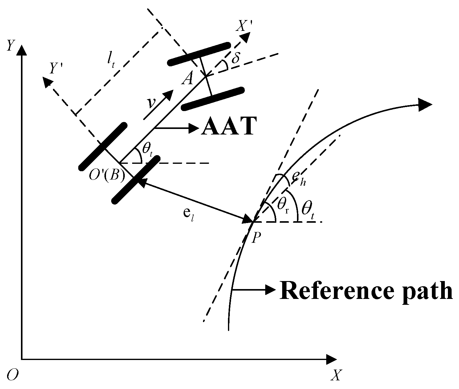
2.1. Symbol Definition and Issue Description

To simplify analysis, the model of a vehicle is replaced by an ideal tractor model, and the comprehensive path tracking model is shown in Figure 1. The turning is controlled by the front wheel steering system, which is relevant to the steering angle. Its motive force is generated by the lateral wheels, and a coordinate system of $O^{\prime }{X}^{\prime }{Y}^{\prime }$ is affixed to the central point B on the lateral axle. On the basis of it, some key variables are summarized in

Table 1. The description and dimension of the parameters and variables.

Notations	Descriptions	Dimension
$e_l$	Lateral offset	-/m
$e_h$	Heading offset	-/rad
$\delta$	Turning angle of front wheel	-/rad
$l_t$	Wheelbase	0.9 m
${\theta }_t$	Real angle of AAT	-/rad
${\theta }_r$	Planned angle at tracking point	-/rad
v	Velocity of AAT	1 m/s
$c_r$	Curvature of reference path	-

.

Generally, the primary objective in resolving the path tracking problem for the AATs is to design an appropriate controller u (related to the front wheel steering angle $\delta$ in this paper), ensuring that the lateral offset $e_l$ and the heading offset $e_h$ approach zero.

2.2. Ideal Model

Suppose that the angles are positive when measured in the anticlockwise direction. The ideal model of the AAT is established below:

$$\begin{array}{c}\hfill {\dot{x}}_t=v\cos {\theta }_t,{\dot{y}}_t=v\sin {\theta }_t,{\dot{\theta }}_t={\displaystyle \frac{v}{l_t}}\tan \delta \end{array}$$

(1)

among which $x_t$ and $y_t$ represent the vehicle’s positional coordinates, ${\theta }_t$ denotes its orientation, and $\delta$ is the steering angle of the front wheels, which is the only variable that can be controlled. v is positive when the vehicle moves forward, and it is negative otherwise. $l_t$ is the wheelbase of the AAT.

2.3. Offset Model

The offset model of the AAT in this paper can be described as follows:

$$\left\{\begin{array}{l}{\dot{e}}_l=-\beta \left|v\right|\sin e_h\\ {\dot{e}}_h={\displaystyle \frac{v}{l_t}}\tan \delta -\beta \left|v\right|{\displaystyle \frac{c_r\cos e_h}{1+c_r{e}_l}}.\end{array}\right.$$

(2)

where $c_r$ is the unknown curvation of the path, $\beta =1$ when the AAT is moving with an anticlockwise rotation, and $\beta =-1$ when the AAT is moving with a clockwise rotation. Specifically, in this paper, the AAT is assumed to be moving toward steadily and tracks the planned path in the direction of a clockwise rotation. Under this circumstance, the sign parameter $\beta$ in (2) is equal to $-1$, and v is greater than 0. Based on the above mentioned assumption, by defining $x_1=e_l$, $x_2=v\sin e_h$, $u=\tan \delta$, the offset model (2) can be further rewritten as follows:

$$\left\{\begin{array}{l}{\dot{x}}_1=x_2\\ {\dot{x}}_2={\displaystyle \frac{v^2{c}_r\left(1-\frac{x_2^2}{v^2}\right)}{1+c_r{x}_1}}+{\displaystyle \frac{v^2{\left(1-\frac{x_2^2}{v^2}\right)}^{\frac{1}{2}}}{l_t}}u\end{array}\right.$$

(3)

where $x_1,x_2\in {\mathbb{R}}^2$ are two states that can describe the motion state of the entire system; $u\in \mathbb{R}$ is the controller.

In order to design a state observer to deal with $x_2$ for the unknown heading offset, we can reformulate ${\dot{x}}_2$ below:

$$\begin{array}{cc}\hfill {\dot{x}}_2& ={\displaystyle \frac{v^2{c}_r}{1+c_r{x}_1}}-{\displaystyle \frac{c_r{x}_2^2}{1+c_r{x}_1}}+{\displaystyle \frac{v^2}{l_t}}u+{\displaystyle \frac{v^2}{l_t}}\left[{\left(1-{\displaystyle \frac{x_2^2}{v^2}}\right)}^{{\displaystyle \frac{1}{2}}}-1\right]u=\chi u+g(x,t)\hfill \end{array}$$

(4)

where $\chi ={\displaystyle \frac{v^2}{l_t}}$, and $g(x,t)$ denotes the unknown term, expressed below:

$$\begin{array}{c}\hfill g(x,t)={\displaystyle \frac{v^2{c}_r-c_r{x}_2^2}{1+c_r{x}_1}}+{\displaystyle \frac{v^2}{l_t}}\left[{(1-{\displaystyle \frac{x_2^2}{v^2}})}^{{\displaystyle \frac{1}{2}}}-1\right]u.\end{array}$$

(5)

Under these circumstances, the original offset dynamics Equation (3) can be reformulated as shown below:

$$\left\{\begin{array}{l}{\dot{x}}_1=x_2\\ {\dot{x}}_2=\chi u+g(x,t).\end{array}\right.$$

(6)

Normally, the unknown part $g(x,t)$ necessitates the additional assumption, as detailed below.

Assumption A1.

A constant $w\ge 0$ exists such that

$$\begin{array}{c}\hfill g(x,t)=\left|{\displaystyle \frac{v^2{c}_r-c_r{x}_1^2}{1+c_r{x}_2}}+{\displaystyle \frac{v^2}{l_t}}\left[{\left(1-{\displaystyle \frac{x_1^2}{v^2}}\right)}^{{\displaystyle \frac{1}{2}}}-1\right]u\right|\le w\left(\left|x_1\left(t\right)\right|+\left|x_2\left(t\right)\right|\right).\end{array}$$

(7)

It is worth noting that the system’s stability inherently implies the boundedness of all state and control parameters. Based on this fundamental linkage between stability and parameter boundedness, it can be logically inferred that a sufficiently large w is mathematically guaranteed to ensure the validity of this assumption.

Under Assumption 1, the authors in [35] proved that the stabilization for (6) is feasible using state feedback. Later, ref. [36] showed that using the linear output feedback method can also be used to achieve global stability. Nevertheless, the design processes of the controllers are carried out on the basis of the continuous system. The purpose of this paper is to design a discrete-time observer-based sampled-data output feedback controller for system (6), which can save the cost of the AAT and constrain the effect of the long sampling period.

3. Control Design

This section is dedicated to the design of the sampled-data controller that stabilizes system (6). The theorem is given below.

Theorem 1.

Based on Assumption 1, if the controller and the observer are designed as

$$\left\{\begin{array}{cc}\hfill u\left(t\right)& =u\left(t_{\tau }\right)=-L_1{\widehat{x}}_1\left(t_{\tau }\right)-L_2{\widehat{x}}_2\left(t_{\tau }\right),\hfill \\ \hfill {\dot{\widehat{x}}}_1\left(t\right)& =\mu {\widehat{x}}_2\left(t\right)+\mu {\alpha }_1(x_1\left(t_{\tau }\right)-{\widehat{x}}_1\left(t\right)),\hfill \\ \hfill {\dot{\widehat{x}}}_2\left(t\right)& =\chi \mu u\left(t_{\tau }\right)+{\mu }^2{\alpha }_2(x_1\left(t_{\tau }\right)-{\widehat{x}}_1\left(t\right)),\forall t\in [t_{\tau },t_{\tau +1}]\hfill \end{array}\right.$$

(8)

among which ${\widehat{x}}_1\left(t\right)$ and ${\widehat{x}}_2\left(t\right)$ are the estimations of $x_1\left(t\right)$, $x_2\left(t\right)$, $L_1={\displaystyle \frac{k_1\mu }{\chi }}$ and $L_2={\displaystyle \frac{k_2\mu }{\chi }}$, $k_1,k_2>0$ satisfy the Hurwitz polynomial $p_1\left(s\right)=s^2+k_{2}s+k_1$; ${\alpha }_1$ and ${\alpha }_2$ are the same conditions satisfying the Hurwitz polynomial $p_2\left(s\right)=s^2+{\alpha }_{2}s+{\alpha }_1$, and μ is the gain. Thus, the AAT system (6) can be stabilized.

Proof. 

The proof of Theorem 1 is divided into the following four steps.

Step 1. Pre-Treatment of System (6): Change of coordinates

First of all, a transformation of coordinates is implemented, which will transform the system into the form of output feedback control. Define a gain $\mu \ge 1$, and the changes are as follows:

$$\begin{array}{c}\hfill z_1=x_1,z_2={\displaystyle \frac{x_2}{\mu }},\mathrm{and}v={\displaystyle \frac{\chi u}{\mu }}.\end{array}$$

(9)

Based on this transformation of coordinates, system (6) undergoes the following changes:

$$\left\{\begin{array}{l}{\dot{z}}_1\left(t\right)=\mu z_2\\ \dot{z_2}\left(t\right)=\mu v\left(t\right)+\overline{g}(z,t)\\ y\left(t\right)=C_{0}z\left(t\right)\end{array}\right.$$

(10)

where $\overline{g}(z,t)={\displaystyle \frac{g(x,t)}{\mu }}$.

Under Assumption 1, it can be verified that

$$\begin{array}{c}\hfill |\overline{g}(z,t)|\le {\displaystyle \frac{w}{\mu }}\left(|z_1\left(t\right)|+|\mu z_2\left(t\right)|\right)\le w\left(|z_1\left(t\right)|+|z_2\left(t\right)|\right).\end{array}$$

(11)

Define

$$z\left(t\right)=\left[\begin{array}{c}{z}_1\left(t\right)\\ z_2\left(t\right)\end{array}\right],A_0=\left[\begin{array}{cc}0& 1\\ 0& 0\end{array}\right],J=\left[\begin{array}{c}0\\ 1\end{array}\right],C_0=\left[\begin{array}{cc}1& 0\end{array}\right],\overline{G}(·)=\left[\begin{array}{c}0\\ \overline{g}(z,t)\end{array}\right]$$

under which (10) can be changed to

$$\left\{\begin{array}{l}\dot{z}\left(t\right)=\mu A_{0}z\left(t\right)+\mu Jv\left(t\right)+\overline{G}(·)\\ y\left(t\right)=C_{0}z\left(t\right).\end{array}\right.$$

(12)

The following proof will be proposed on the basis of (12). Given that only $y=z_1$ can be measured, a state observer will be constructed for $z_2$.

Step 2. Design of the observer

Firstly, drawing on the continuous-time observer from [35,36], the following state observer is constructed, including continuous states over $[t_{\tau },t_{\tau +1}]$ and discrete ones $z_1\left(t_{\tau }\right)$ and $v\left(t_{\tau }\right)$:

$$\left\{\begin{array}{l}{\dot{\widehat{z}}}_1\left(t\right)=\mu {\widehat{z}}_2\left(t\right)+\mu {\alpha }_1(z_1\left(t_{\tau }\right)-{\widehat{z}}_1\left(t\right)),\\ {\dot{\widehat{z}}}_2\left(t\right)=\mu v\left(t_{\tau }\right)+\mu {\alpha }_2(z_1\left(t_{\tau }\right)-{\widehat{z}}_1\left(t\right)),\forall t\in [t_{\tau },t_{\tau +1}).\end{array}\right.$$

(13)

By defining the following arrows and the matrices $\widehat{z}\left(t\right)=[{\widehat{z}}_1\left(t\right)$, ${\widehat{z}}_2{\left(t\right)]}^T$, $D={[{\alpha }_1,{\alpha }_2]}^T$ and $\mathbb{A}=A_0-D{C}_0$, observer (13) can be shown as

$$\begin{array}{c}\hfill \dot{\widehat{z}}\left(t\right)=\mu \mathbb{A}\widehat{z}\left(t\right)+\mu Jv\left(t_{\tau }\right)+\mu D{z}_1\left(t_{\tau }\right),\forall t\in [t_{\tau },t_{\tau +1}).\end{array}$$

(14)

If the time is discrete, the continuous observer (13) will own the following form:

$$\begin{array}{c}\hfill \widehat{z}\left(t_{\tau +1}\right)=(F-G\mathcal{K})\widehat{z}\left(t_{\tau }\right)+N{z}_1\left(t_{\tau }\right)=M\widehat{z}\left(t_{\tau }\right)+Ny\left(t_{\tau }\right)\end{array}$$

(15)

where $F=e^{\mu \mathbb{A}T}$, $G={\int }_0^T{e}^{\mu \mathbb{A}s}ds\mu J$, $N={\int }_0^T{e}^{\mu \mathbb{A}s}ds\mu D$, and $v\left(t_{\tau }\right)=-\mathcal{K}\widehat{z}\left(t_{\tau }\right)$; $\mathcal{K}$ will be defined in the following part.

Step 3. Design of a sampled-data output feedback controller

The controller uses the estimated states, and the form of the controller is constructed below:

$$\begin{array}{cc}\hfill v\left(t\right)=v\left(t_{\tau }\right)={\displaystyle \frac{\chi }{\mu }}u\left(t\right)& =-k_1{\widehat{z}}_1\left(t_{\tau }\right)-k_2{\widehat{z}}_2\left(t_{\tau }\right)=-\mathcal{K}\widehat{z}\left(t_{\tau }\right),\forall t\in [t_k,t_{\tau +1}).\hfill \end{array}$$

(16)

By inserting the controller (16) into systems (12) and (14), it can be obtained that the form of the close-loop system during the time span $[t_k,t_{\tau +1})$ is transformed as follows:

$$\begin{array}{c}\hfill \left[\begin{array}{c}\dot{z}\left(t\right)\\ \dot{\widehat{z}}\left(t\right)\end{array}\right]=\mu \left[\begin{array}{cc}{A}_0& 0\\ 0& \mathbb{A}\end{array}\right]\left[\begin{array}{c}z\left(t\right)\\ \widehat{z}\left(t\right)\end{array}\right]-\mu \left[\begin{array}{c}J\\ J\end{array}\right]K\widehat{z}\left(t_{\tau }\right)+\mu \left[\begin{array}{c}0\\ D\end{array}\right]z_1\left(t_{\tau }\right)+\left[\begin{array}{c}\overline{g}(z,t)\\ 0\end{array}\right].\end{array}$$

(17)

Since $z_1\left(t_{\tau }\right)=C_{0}z\left(t_{\tau }\right)=C_{0}z\left(t\right)+C_0(z\left(t_{\tau }\right)-z\left(t\right))$ and $\widehat{z}\left(t_{\tau }\right)=\widehat{z}\left(t\right)+\widehat{z}\left(t_{\tau }\right)-\widehat{z}\left(t\right)$, system (17) can be changed to the following form:

$$\begin{array}{cc}\hfill \left[\begin{array}{c}\dot{z}\left(t\right)\\ \dot{\widehat{z}}\left(t\right)\end{array}\right]& =\mu \left[\begin{array}{cc}{A}_0& -J\mathcal{K}\\ DC& \mathbb{A}-J\mathcal{K}\end{array}\right]\left[\begin{array}{c}z\left(t\right)\\ \widehat{z}\left(t\right)\end{array}\right]-\mu \left[\begin{array}{c}J\\ J\end{array}\right]\mathcal{K}(\widehat{z}\left(t_{\tau }\right)-\widehat{z}\left(t\right))\hfill \\ & +\mu \left[\begin{array}{c}0\\ D\end{array}\right]C_0(z\left(t_{\tau }\right)-z\left(t\right))+\left[\begin{array}{c}\overline{g}(z,t)\\ 0\end{array}\right],\forall t\in [t_{\tau },t_{\tau +1})\hfill \end{array}$$

(18)

and $\mathcal{A}=\left[\begin{array}{cc}{A}_0& -J\mathcal{K}\\ D{C}_0& \mathbb{A}-J\mathcal{K}\end{array}\right]=\left[\begin{array}{cc}{A}_0& -J\mathcal{K}\\ D{C}_0& A_0-D{C}_0-J\mathcal{K}\end{array}\right]$.

By combining with the relation

$$\mathcal{A}=\left[\begin{array}{cc}{A}_0& -J\mathcal{K}\\ D{C}_0& A_0-D{C}_0-J\mathcal{K}\end{array}\right]={\left[\begin{array}{cc}I& 0\\ -I& I\end{array}\right]}^{-1}\left[\begin{array}{cc}{A}_0-J\mathcal{K}& -J\mathcal{K}\\ 0& \mathbb{A}\end{array}\right]\left[\begin{array}{cc}I& 0\\ -I& I\end{array}\right],$$

it can be concluded that $\mathcal{A}$ is a Hurwitz matrix as well. Hence, there is a positive definite matrix $U=U^T\in {\mathbb{R}}^{2n\times 2n}>0$ such that ${\mathcal{A}}^{T}U+U\mathcal{A}=-I$. Construct the Lyapunov function $V\left(\mathbb{Z}\right)={\mathbb{Z}}^{T}U\mathbb{Z}$ with $\mathbb{Z}\left(t\right)=\left[\begin{array}{c}z\left(t\right)\\ \widehat{z}\left(t\right)\end{array}\right]$, and $\dot{V}\left(\mathbb{Z}\right)$ is as follows:

$$\begin{array}{cc}\hfill \dot{V}\left(\mathbb{Z}\left(t\right)\right)& =-\mu {∥\mathbb{Z}\left(T\right)∥}^2+2\mathbb{Z}{\left(t\right)}^{T}U\left[\begin{array}{c}\overline{g}(z,t)\\ 0\end{array}\right]+2\mu \mathbb{Z}{\left(t\right)}^{T}U\left[\begin{array}{c}J\\ J\end{array}\right]\mathcal{K}(\widehat{z}\left(t_{\tau }\right)-\widehat{z}\left(t\right))\hfill \\ & +2\mu \mathbb{Z}{\left(t\right)}^{T}U\left[\begin{array}{c}0\\ D\end{array}\right](z_1\left(t_{\tau }\right)-z_1\left(t\right)),\forall t\in [t_{\tau },t_{\tau +1}).\hfill \end{array}$$

(19)

In the next step, the work will concentrate on the selection of the gain $\mu$ and sampling period T, and by using the selected parameters, system (17) can be stabilized.

Step 4. Stability analysis and parameter selection

To select $\mu$ and T, it is essential to estimate several terms in (19). Firstly, we consider the second term on the right side of (19). Based on (11), the following inequality holds:

$$\begin{array}{c}\hfill ∥\overline{g}(z,t)∥\le w\sqrt{z_1^2+z_2^2}\le w_1\parallel \mathbb{Z}\left(t\right)\parallel ,\end{array}$$

(20)

where $w_1=\sqrt{3}w>0$. Using (19), it has

$$\begin{array}{c}\hfill \left|2\mathbb{Z}{\left(t\right)}^{T}U\left[\begin{array}{c}\overline{g}(z,t)\\ 0\end{array}\right]\right|\le 2w_1{\lambda }_{max}\left(U\right){\parallel \mathbb{Z}\left(t\right)\parallel }^2.\end{array}$$

(21)

Then, the latter two parts will be approximated. Firstly, through ${\dot{z}}_1\left(t\right)=L{z}_2\left(t\right)+{\overline{g}}_1(z,t)$, it can be concluded that

$$\begin{array}{c}\hfill |{\dot{z}}_1\left(\tau \right)|\le \mu |z_2\left(\tau \right)+w|z_1\left(\tau \right)\le \mu {\displaystyle \frac{\sqrt{2}(w+1)}{\sqrt{{\lambda }_{min}\left(U\right)}}}\sqrt{V\left(\mathbb{Z}\right(\tau \left)\right)}.\end{array}$$

(22)

By combining with (20), it can be concluded that

$$\begin{array}{c}\hfill |z_1\left(t_{\tau }\right)-z_1\left(t\right)|\le {\int }_{t_{\tau }}^t|{\dot{z}}_1\left(u\right)du\le \mu w_2\sqrt{V_{max}\left(t\right)}(t-t_{\tau })\end{array}$$

(23)

where $w_3={\displaystyle \frac{\sqrt{2}(w+1)}{\sqrt{{\lambda }_{min}\left(U\right)}}}$ and $V_{max}\left(t\right)=maxV(\mathbb{Z}\left(u\right),\forall u\in [t_{\tau },t_{\tau +1})$.

At last, we estimate $\mathcal{K}(\widehat{z}\left(t_{\tau }\right)-\widehat{z}\left(t\right))$. Note that

$$\begin{array}{c}\hfill |\mathcal{K}(\widehat{z}\left(t_{\tau }\right)-\widehat{z}\left(t\right))|\le {\int }_{t_{\tau }}^t|\mathcal{K}\dot{\widehat{z}}\left(u\right)du.\end{array}$$

(24)

By (14) and (16), for any $u\in [t_{\tau },t_{\tau +1})$,

$$\begin{array}{c}\hfill \left|\mathcal{K}\dot{\widehat{z}}\left(u\right)\right|=|\mathcal{K}\mu \mathbb{A}\widehat{z}\left(u\right)-\mathcal{K}\mu J\mathcal{K}\widehat{z}\left(t_{\tau }\right)+\mathcal{K}\mu D{z}_1\left(t_{\tau }\right)|\le \mu w_2\sqrt{V_{max}\left(t\right)}\end{array}$$

(25)

where $w_2={\displaystyle \frac{(\parallel \mathcal{K}\mathbb{A}+\parallel {\mathcal{K}}^{T}J\mathcal{K}\parallel +\parallel \mathcal{K}D\parallel )}{\sqrt{{\lambda }_{min}\left(U\right)}}}$. On the basis of (23) and (24), the following equation is obtained:

$$\begin{array}{c}\hfill |\mathcal{K}(\widehat{z}\left(t_{\tau }\right)-\widehat{z}\left(t\right))|\le \mu w_2\sqrt{V_{max}\left(t\right)}(t-t_{\tau }).\end{array}$$

(26)

Substituting (21), (23), and (24) into (19) results in

$$\begin{array}{cc}\hfill \dot{V}\left(\mathbb{Z}\left(t\right)\right)& \le -{\mu \parallel \mathbb{Z}\left(t\right)\parallel }^2+2w_1{\lambda }_{max}\left(U\right)\parallel \mathbb{Z}{\left(t\right)}^2]\hfill \\ \hfill & +2w_2{\mu }^2\parallel \mathbb{Z}\left(t\right)\parallel ∥U\left[\begin{array}{c}J\\ J\end{array}\right]∥\sqrt{V_{max}\left(t\right)}(t-t_{\tau })\hfill \\ & +2w_3{\mu }^2\parallel \mathbb{Z}\left(t\right)\parallel ∥U\left[\begin{array}{c}0\\ D\end{array}\right]∥\sqrt{V_{max}\left(t\right)}(t-t_{\tau }).\hfill \end{array}$$

(27)

Noting that $\parallel J\parallel =1$, $\parallel U\parallel ={\lambda }_{max}\left(U\right)$, and $\parallel \mathbb{Z}\left(t\right)\parallel \le \sqrt{{\displaystyle \frac{V\left(\mathbb{Z}\right(t\left)\right)}{{\lambda }_{min}\left(U\right)}}}$, (27) can be transformed to the form

$$\begin{array}{cc}\hfill \dot{V}\left(\mathbb{Z}\left(t\right)\right)& \le -(\mu -2w_1{\lambda }_{max}\left(U\right)){\parallel \mathbb{Z}\left(t\right)\parallel }^2\hfill \\ & +{\mu }^2{w}_4\sqrt{V\left(\mathbb{Z}\right(t\left)\right)}\sqrt{V_{max}\left(t\right)}(t-t_{\tau }),t\in [t_k,t_{\tau +1})\hfill \end{array}$$

(28)

where $w_4={\displaystyle \frac{2(\sqrt{2}{w}_3+\parallel D\parallel w_2){\lambda }_{max}\left(U\right)}{\sqrt{{\lambda }_{min}\left(U\right)}}}=2[\sqrt{2}(\parallel \mathcal{K}\mathbb{A}\parallel +\parallel \mu J\mathcal{K}\parallel +\parallel \mathcal{K}D\parallel )+\parallel D\parallel ]{\displaystyle \frac{{\lambda }_{max}\left(U\right)}{{\lambda }_{min}\left(U\right)}}$.

Based on (28), the two parameters $\mu$ and T can now be selected as

$$\begin{array}{c}\hfill \mu \ge 2w_1{\lambda }_{max}\left(U\right)+w^{*},{\mu }^2{w}_4{\lambda }_{max}\left(U\right)T<w^{*},w^{*}>0,\end{array}$$

(29)

so that the system can achieve the global stability. In the analysis below, we will utilize the relationship (28) in conjunction with (29) to prove that

$$\begin{array}{c}\hfill maxV\left(\mathbb{Z}\left(u\right)\right)=V\left(\mathbb{Z}\left(t_{\tau }\right)\right),\forall u\in [t_{\tau },t_{\tau +1}).\end{array}$$

(30)

If (30) does not hold, it is obvious that a time instant $t^{\prime }\in [t_{\tau },t_{\tau +1})$ exists such that $V\left(\mathbb{Z}\left(t^{\prime }\right)\right)>V\left(\mathbb{Z}\left(t_{\tau }\right)\right)$. By $\mu >2w_1{\lambda }_{max}\left(U\right)$ in (29), it can be proved from (28) that for $\mathbb{Z}\left(t_{\tau }\right)\ne 0,\dot{V}\left(\mathbb{Z}\left(t_{\tau }\right)\right)<0$ holds, which implies that $V\left(\mathbb{Z}\right(t\left)\right)$ will decrease in a short time starting from $t_{\tau }$. Hence, there is a time instant $t″\in [t_{\tau },t^{\prime }]$ such that

$$\begin{array}{c}\hfill \left\{\begin{array}{c}\left(i\right)V\left({\mathbb{Z}}_n(t″)\right)=V\left({\mathbb{Z}}_n\left(t_{\tau }\right)\right)\hfill \\ \left(ii\right)\dot{V}\left(\mathbb{Z}(t″)\right)>0\hfill \\ \left(iii\right)V\left({\mathbb{Z}}_n\left(t\right)\right)\le V\left({\mathbb{Z}}_n\left(t_{\tau }\right)\right),\forall t\in [t_{\tau },t″].\hfill \end{array}\right.\end{array}$$

(31)

On the basis of relations (28) and (31), the following holds:

$$\begin{array}{cc}\hfill \dot{V}(\mathbb{Z}(t″))& \le -(\mu -2w_1{\lambda }_{max}(U)){\parallel \mathbb{Z}(t″)\parallel }^2+{\mu }^2{w}_4\sqrt{V(\mathbb{Z}(t″))}·\sqrt{V(\mathbb{Z}(t″))}T\hfill \\ & \le -(\mu -2w_1{\lambda }_{max}(U))-{\mu }^2{w}_4{\lambda }_{max}(U)T{\parallel \mathbb{Z}(t″)\parallel }^2<0\hfill \end{array}$$

(32)

and it conflicts with the assumption. Therefore, (30) holds.

Given this result, it follows from (28) that

$$\begin{array}{cc}\hfill \dot{V}\left(\mathbb{Z}\left(t\right)\right)& \le -(\mu -2w_1{\lambda }_{max}\left(U\right)){\displaystyle \frac{V\left(\mathbb{Z}\right(t\left)\right)}{{\lambda }_{max}\left(U\right)}}\hfill \\ & +T{\mu }^2{w}_4\sqrt{V\left(\mathbb{Z}\right(t\left)\right)}·\sqrt{V\left(\mathbb{Z}\left(t_{\tau }\right)\right)},\forall t\in [t_{\tau },t_{\tau +1}).\hfill \end{array}$$

(33)

Let $\zeta \left(t\right)=\sqrt{{\displaystyle \frac{V\left(\mathbb{Z}\right(t\left)\right)}{V\left(\mathbb{Z}\left(t_{\tau }\right)\right)}}}$; thus, it can be concluded that

$$\dot{\zeta }\left(t\right)\le -{\displaystyle \frac{1}{2}}(\mu -2w_1{\lambda }_{max}\left(U\right))\zeta \left(t\right)+{\displaystyle \frac{1}{2}}T{\mu }^2{w}_4,\forall t\in [t_{\tau },t_{\tau +1}).$$

Noticing that $\zeta \left(t_{\tau }\right)=1$, we have

$$\begin{array}{c}\hfill \zeta \left(t_{\tau +1}\right)\le e^{-{\displaystyle \frac{1}{2}}(\mu -2w_1{\lambda }_{max}\left(U\right))T}+[1-e^{-{\displaystyle \frac{1}{2}}(\mu -2w_1{\lambda }_{max}\left(U\right))T}]{\displaystyle \frac{T{\mu }^2{w}_4{\lambda }_{max}\left(U\right)}{\mu -2w_1{\lambda }_{max}\left(U\right)}}=\rho \end{array}$$

(34)

implying that $V\left(\mathbb{Z}(t_{\tau }+1)\right)\le {\rho }^{2}V\left(\mathbb{Z}\left(t_{\tau }\right)\right)$.

From (29), it can be deduced that ${\displaystyle \frac{T{\mu }^2{w}_4{\lambda }_{max}\left(U\right)}{\mu -2w_1{\lambda }_{max}\left(U\right)}}<1$; from this, it follows that the constant $\rho <1$. Thus, $V\left(\mathbb{Z}\left(t_{\tau }\right)\right)$ approaches zero. In conclusion, the controller and the observer constructed as (16) can stabilize the AAT system (6). Moreover, by applying the inverse coordinate transformation, the result of Theorem 1 can be proved. □

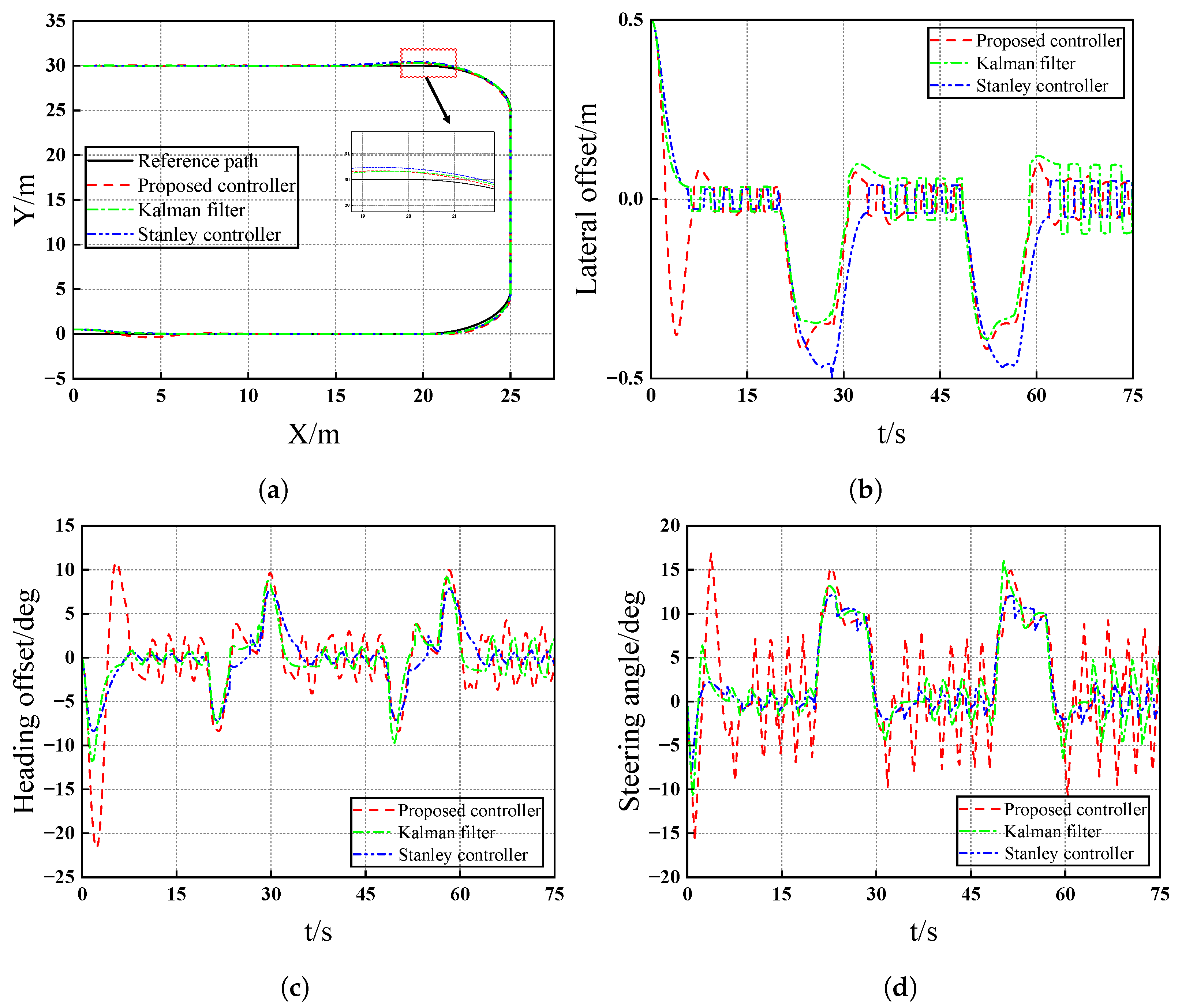
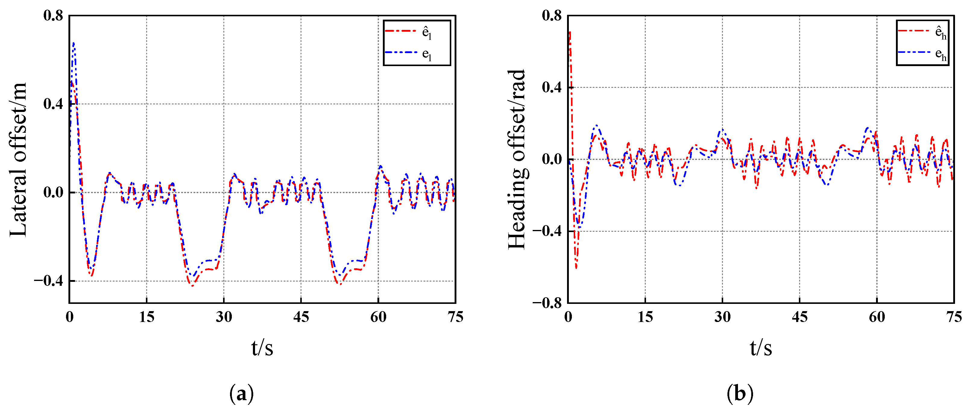
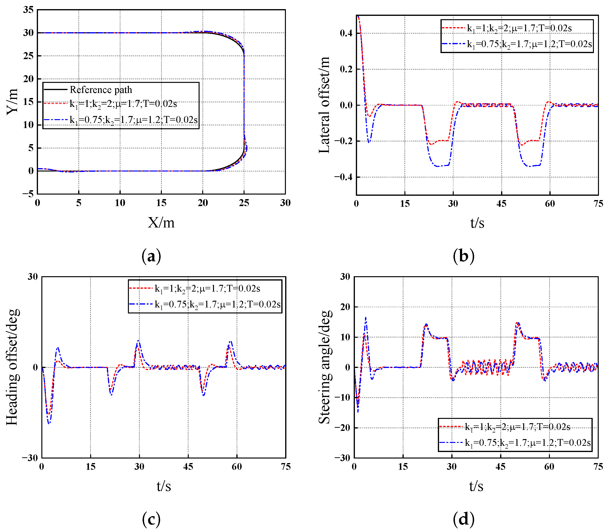
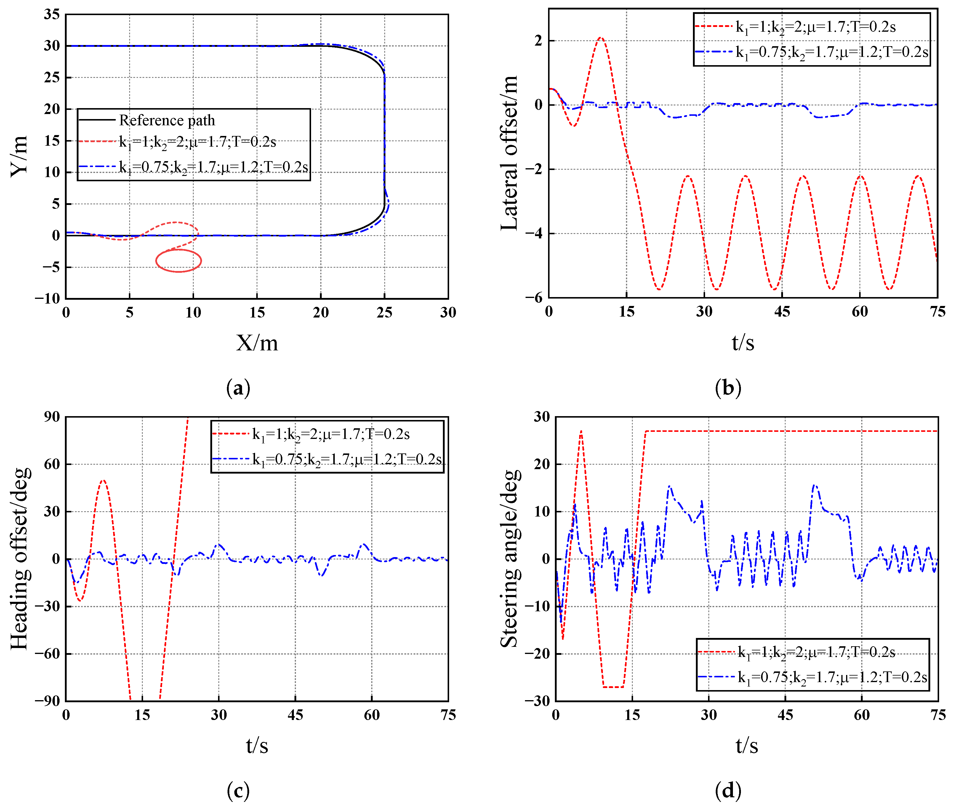
4. Simulation Results

Consider system (6). It is clear that the nonlinearity $g(x,t)$ satisfies the assumption. As a matter of fact, by changing the coordinates $z_1=x_1$ and $z_2={\displaystyle \frac{x_2}{\mu }}$, and in combination with Theorem 1, the controller can be formulated as follows:

$$\begin{array}{cc}\hfill \widehat{z}\left(t_{\tau +1}\right)& =M\widehat{z}\left(t_{\tau }\right)+Ny\left(t_{\tau }\right),M\in {\mathbb{R}}^{2\times 2},N\in {\mathbb{R}}^{2\times 1}\hfill \\ \hfill u\left(t\right)& =u\left(t_{\tau }\right)=-{\displaystyle \frac{\mu }{\chi }}v\left(t_{\tau }\right)=-{\displaystyle \frac{\mu }{\chi }}(k_1{\widehat{z}}_1\left(t_{\tau }\right)+k_2{\widehat{z}}_2\left(t_{\tau }\right)),\forall t\in [t_k,t_{\tau +1})\hfill \end{array}$$

(35)

with appropriately coefficients. The parameters for the proposed controller are selected as $k_1=0.75$, $k_2=1.7$, and $\mu =1.2$, and we have a sampling period $T=0.2$ s. Therefore, $M=\left[\begin{array}{cc}0.4868& -0.2468\\ -1.0011& 0.4955\end{array}\right]$, $N=\left[\begin{array}{c}1.2984\\ 1.1143\end{array}\right]$.

To demonstrate the effectiveness of the controller, the other two control methods are selected, including the Stanley control method and the Kalman filter-based control method. The form of the Stanley control method was proposed in [37], and the Kalman filter-based method was proposed in [38,39]. The parameter of the Stanley control method is selected as $k=0.6$, and the initial states of the Kalman filter reported in [38,39] are selected as $A=\left[\begin{array}{ccc}1& 0.2& 0\\ 0& 1& 0.2\\ 0& 0& 1\end{array}\right]$, $B=\left[\begin{array}{c}0\\ {\displaystyle \frac{2}{9}}\\ 0\end{array}\right]$, $H=\left[\begin{array}{ccc}1& 0& 0\\ 0& 1& 0\end{array}\right]$, $P=\left[\begin{array}{ccc}0.1& & \\ & 0.1& \\ & & 0.01\end{array}\right]$, $Q=\left[\begin{array}{ccc}0.01& & \\ & 0.01& \\ & & 0.001\end{array}\right]$, and $R=\left[\begin{array}{cc}0.1& \\ & 0.1\end{array}\right]$. The axle length is $0.9$ m, with a longitudinal velocity of 1 m/s. The desired route is chosen as a U-shaped line. The AAT is initialized with the condition ${(x_t\left(0\right),y_t\left(0\right),{\theta }_t\left(0\right))}^T={(0,0.5,0)}^T$. The starting value for the observer is ${\widehat{z}}_1\left(0\right)={\widehat{z}}_2\left(0\right)=0$. The simulation results are presented in Figure 2 and Figure 3.

From Figure 2a, it can be observed that all the controllers achieve a certain level of effectiveness in tracking the reference path. It should be noted that, at the turning points, the Kalman filter-based controller exhibits better performance than the proposed controller, while the tracking accuracy on the straight line is too low. On the contrary, the Stanley controller owns a good tracking accuracy on the straight line, but the lateral offset on the curve line is larger than that under the proposed controller. In terms of Figure 2b, the proposed controller maintains a relatively small lateral offset within a narrow range for most of the time. This indicates that the proposed controller has excellent stability and tracking accuracy in lateral offset control. Conversely, the Stanley controller shows the largest lateral offset fluctuations on the curve line, and the Kalman filter-based controller shows excellent tracking results on the curve line, while the lateral offset is too large on the straight line. The heading offset analysis in Figure 2c reveals that the heading offset under the proposed controller is relatively small and occurs in a regular pattern, demonstrating the effectiveness of the controller in adjusting the direction to maintain the consistency with the reference path. Regarding steering angles, as shown in Figure 2d, the steering angle variations under the three controllers are relatively smooth, with the smaller fluctuations being within an appropriate range.

Moreover, the efficacy of the observer is demonstrated in Figure 3. Specially, in Figure 3a, the estimation of the lateral offset and the real value over time is shown. The results indicate that the estimated values closely follow the actual values across the duration of the simulation. Similarly, Figure 3b presents the heading offset over time. The estimated heading offset values closely match the actual values as well, showing the observer’s capability to accurately track the heading offset of the AAT.

Finally, the impact on the AAT resulting from different frequencies of the GPS-RTK system is demonstrated in the following comparative simulation. The two coupled sets of parameters are shown in

Table 2. The set for the parameters.

Couple	Parameters Choice
Couple 1	$k_1=1$; $k_2=2$; $\mu =1.7$
Couple 2	$k_1=0.75$; $k_2=1.7$; $\mu =1.2$

.

The simulation results are depicted in Figure 4 and Figure 5. In the first figure with a 0.02 s sampling period, Couple 1 parameters achieve better tracking performances than Couple 2 parameters. However, in the second figure using a 0.2 s sampling period, the path tracking trajectories under the parameter conditions of Couple 1 diverge, while the the path tracking trajectories under the parameter conditions of Couple 2 remain stable. This demonstrates the critical role of the sampling period in determining the parameter selection of the controller and therefore showing that the frequency of the GPS-RTK system significantly influences the tracking performances. This underscores the need for thorough research into sampled-data control to ensure consistent and reliable performance in the AAT path tracking system. On the basis of the analysis above, it is meaningful to investigate sampled-data control, thereby ensuring consistent and reliable performance in the AAT path tracking system.

5. Conclusions

In this paper, a composite sampled-data control method based on a state observer was put forward for the AAT. Considering the influence caused by the low frequency of the GPS-RTK system, a sampled-data control algorithm was proposed. On the foundation of the designed observer, a sample-data controller was developed to tackle the slow data refresh resulting from the low sampling frequency of the GPS-RTK system and ensure the stability of the AAT system. It should be noticed that our proposed method is particularly suitable for systems with low-data update frequencies and low device configurations. This is because a larger sampling period can reduce the update frequency, thereby alleviating the computational burden on the controller. However, we also acknowledge that this smooth controller has certain limitations, such as a relatively slow response speed and sensitivity to disturbance variations. Therefore, our further research will focus on handling these problems.

References

1. Shi, Q.; Liu, D.; Mao, H.; Shen, B.; Li, M. Wind-induced response of rice under the action of the downwash flow field of a multi-rotor UAV. Biosyst. Eng. 2021, 203, 60–69. [Google Scholar] [CrossRef]
2. Ji, W.; Pan, Y.; Xu, B.; Wang, J. A Real-Time Apple Targets Detection Method for Picking Robot Based on ShufflenetV2-YOLOX. Agriculture 2023, 12, 856. [Google Scholar] [CrossRef]
3. Sun, J.; Zhang, L.; Zhou, X.; Yao, K.S.; Tian, Y.; Nirere, A. A method of information fusion for identification of rice seed varieties based on hyperspectral imaging technology. J. Food Process. Eng. 2021, 44, 13797. [Google Scholar] [CrossRef]
4. Ding, Z.; Tang, Z.; Zhang, B.; Ding, C. Vibration response of metal plate and shell structure under multi-source excitation with welding and bolt connection. Agriculture 2024, 14, 816. [Google Scholar] [CrossRef]
5. Thanpattranon, P.; Ahamed, T.; Takigawa, T. Navigation of autonomous tractor for orchards and plantations using a laser range finder: Automatic control of trailer position with tractor. Biosyst. Eng. 2016, 147, 90–103. [Google Scholar] [CrossRef]
6. Hu, J.; Gao, L.; Bai, X.; Li, T.; Liu, X. Review of research on automatic guidance of agricultural vehicles. Trans. Chin. Soc. Agric. Eng. 2015, 31, 1–10. [Google Scholar]
7. Chen, C.; Liu, X.Q.; Liu, C.J.; Pan, Q. Development of the precision feeding system for sows via a rule-based expert system. Int. J. Agric. Biol. Eng. 2023, 16, 187–198. [Google Scholar] [CrossRef]
8. Ji, W.; Zhang, T.; Xu, B.; He, G. Apple recognition and picking sequence planning for harvesting robot in a complex environment. J. Agric. Eng. 2023, 55, 1549. [Google Scholar] [CrossRef]
9. Backman, J.; Piirainen, P.; Oksanen, T. Smooth turning path generation for agricultural vehicles in headlands. Biosyst. Eng. 2015, 139, 76–86. [Google Scholar] [CrossRef]
10. Zhang, F.; Chen, Z.; Ali, S.; Yang, N.; Fu, S.; Zhang, Y. Multi-class detection of cherry tomatoes using improved YOLOv4-Tiny. Int. J. Agric. Biol. Eng. 2023, 16, 225–231. [Google Scholar] [CrossRef]
11. Zhu, W.; Sun, J.; Wang, S.; Shen, J.; Yang, K.; Zhou, X. Identifying field crop diseases using transformer-embedded convolutional neural network. Agriculture 2022, 12, 1083. [Google Scholar] [CrossRef]
12. Zhu, Y.; Cui, B.; Yu, Z.; Gao, Y.; Wei, X. Tillage Depth Detection and Control Based on Attitude Estimation and Online Calibration of Model Parameters. Agriculture 2024, 14, 2130. [Google Scholar] [CrossRef]
13. Ji, W.; Wang, J.; Xu, B.; Zhang, T. Apple Grading Based on Multi-Dimensional View Processing and Deep Learning. Foods 2023, 12, 2117. [Google Scholar] [CrossRef] [PubMed]
14. Chang, X.H.; Liu, Y.; Shen, M. Resilient control design for lateral motion regulation of intelligent vehicle. IEEE/ASME Trans. Mechatron. 2019, 24, 2488–2497. [Google Scholar] [CrossRef]
15. Lenain, R.; Deremetz, M.; Braconnier, J.B.; Thuilot, B.; Rousseau, V. Robust sideslip angles observer for accurate off-road path tracking control. Adv. Robot. 2017, 31, 453–467. [Google Scholar] [CrossRef]
16. Li, J.; Wu, Z.; Li, M.; Shang, Z. Dynamic Measurement Method for Steering Wheel Angle of Autonomous Agricultural Vehicles. Agriculture 2024, 14, 1602. [Google Scholar] [CrossRef]
17. Lu, E.; Ma, Z.; Li, Y.; Xu, L.; Tang, Z. Adaptive backstepping control of tracked robot running trajectory based on real-time slip parameter estimation. Int. J. Agric. Biol. Eng. 2020, 13, 178–187. [Google Scholar] [CrossRef]
18. Lenain, R.; Thuilot, B.; Cariou, C.; Martinet, P. Adaptive control for car like vehicles guidance relying on RTK GPS: Rejection of sliding effects in agricultural applications. In Proceedings of the International Conference on Robotics and Automation, Taipei, Taiwan, 14–19 September 2003; pp. 115–120. [Google Scholar]
19. Mei, K.; Ding, S.; Dai, X.; Chen, C. Design of second-order sliding-mode controller via output feedback. IEEE Trans. Syst. Man, Cybern. Syst. 2024, 54, 4371–4380. [Google Scholar] [CrossRef]
20. Mei, K.; Ding, S.; Yu, X. A generalized supertwisting algorithm. IEEE Trans. Cybern. 2023, 53, 3951–3960. [Google Scholar] [CrossRef]
21. Sun, J.; Xu, S.; Ding, S.; Pu, Z.; Yi, J. Adaptive conditional disturbance negation-based nonsmooth-integral control for PMSM drive system. IEEE/ASME Trans. Mechatron. 2024, 29, 3602–3613. [Google Scholar] [CrossRef]
22. Li, J.; Shang, Z.; Li, R.; Cui, B. Adaptive Sliding Mode Path Tracking Control of Unmanned Rice Transplanter. Agriculture 2022, 12, 1225. [Google Scholar] [CrossRef]
23. Liu, H.; Yan, S.; Shen, Y.; Li, C.; Zhang, Y.; Hussain, F. Model predictive control system based on direct yaw moment control for 4WID self-steering agriculture vehicle. Int. J. Agric. Biol. Eng. 2021, 14, 175–181. [Google Scholar] [CrossRef]
24. Ding, S.; Zhang, B.; Mei, K.; Park, J.H. Adaptive fuzzy SOSM controller design with output constraints. IEEE Trans. Fuzzy Syst. 2021, 30, 2300–2311. [Google Scholar] [CrossRef]
25. Liu, L.; Ding, S.; Yu, X. Second-order sliding mode control design subject to an asymmetric output constraint. IEEE Trans. Circuits Syst. II Express Briefs 2020, 68, 1278–1282. [Google Scholar] [CrossRef]
26. Yuan, J.; Ding, S.; Mei, K. Fixed-time SOSM controller design with output constraint. Nonlinear Dyn. 2020, 102, 1567–1583. [Google Scholar] [CrossRef]
27. Mei, K.; Liu, J.; Ding, S. Output feedback SOSM control of constrained systems with unmatched uncertainties. IEEE Trans. Autom. Sci. Eng. 2024, 22, 7786–7797. [Google Scholar] [CrossRef]
28. Sun, J.; Wang, Z.; Ding, S.; Xia, J.; Xing, G. Adaptive disturbance observer-based fixed-time nonsingular terminal sliding mode control for path-tracking of unmanned agricultural tractors. Biosyst. Eng. 2024, 246, 96–109. [Google Scholar] [CrossRef]
29. Cui, B.; Cui, X.; Wei, X.; Zhu, Y.; Ma, Z.; Zhao, Y.; Liu, Y. Design and Testing of a Tractor Automatic Navigation System Based on Dynamic Path Search and a Fuzzy Stanley Model. Agriculture 2024, 14, 2136. [Google Scholar] [CrossRef]
30. Li, H.; Mei, K.; Ding, S.; Ding, C.; Sun, J. Sampled-Data Output Feedback Control for Path Tracking of Unmanned Agricultural Vehicles. In Proceedings of the First International Conference on Advanced Robotics, Control, and Artificial Intelligence: ICARCAI 2024, Perth, Australia, 9–12 December 2024; Lecture Notes in Networks and Systems. Springer: Berlin/Heidelberg, Germany, 2025; Volume 1376. [Google Scholar]
31. Qian, C.; Du, H. Global output feedback stabilization of a class of nonlinear systems via linear sampled-data control. IEEE Trans. Autom. Control. 2012, 57, 2934–2939. [Google Scholar] [CrossRef]
32. Zeng, H.B.; Zhai, Z.L.; Xiao, H.Q.; Wang, W. Stability analysis of sampled-data control systems with constant communication delays. IEEE Access 2018, 7, 111–116. [Google Scholar] [CrossRef]
33. Liu, W.; Lim, C.; Shi, P.; Xu, S. Sampled-data fuzzy control for a class of nonlinear systems with missing data and disturbances. Fuzzy Sets Syst. 2017, 306, 63–86. [Google Scholar] [CrossRef]
34. Zhang, W.; Tang, Y.; Zheng, W.; Zou, Y. Stability of Sampled-data systems with packet losses: A nonuniform sampling interval approach. IEEE Trans. Cybern. 2023, 53, 7648–7658. [Google Scholar] [CrossRef] [PubMed]
35. Tsinias, J. A theorem on global stabilization of nonlinear systems by linear feedback. Syst. Control. Lett. 1991, 17, 357–362. [Google Scholar] [CrossRef]
36. Qian, C.; Lin, W. Output feedback control of a class of nonlinear systems: A nonseparation principle paradigm. IEEE Trans. Autom. Control. 2002, 47, 1710–1715. [Google Scholar] [CrossRef]
37. Marsh, A. Past Forward: The Starting Line for Self-Driving Cars: 20 Years Ago, Stanley Won the DARPA Grand Challenge, But the Tech is Still Niche. IEEE Spectr. 2025, 1–4. [Google Scholar]
38. Jin, X.; Chen, W.; Ma, H.; Kong, J.; Su, T.; Bai, Y. Parameter-Free State Estimation Based on Kalman Filter with Attention Learning for GPS Tracking in Autonomous Driving System. Sensors 2023, 23, 8650. [Google Scholar] [CrossRef]
39. Ligeza, P. Reconstructing the trajectory of the object’s motion on the basis of measuring the components of its velocity. Measurement 2023, 221, 113546. [Google Scholar] [CrossRef]
Figure 1. Diagrammatic representation of the path tracking model.
Actuators 14 00300 g001
Figure 2. (a) Path tracking trajectories of the U-shaped curve simulation. (b) Lateral offset of the U-shaped curve simulation. (c) Heading offset of the U-shaped curve simulation. (d) Steering angles of the U-shaped curve simulation.
Actuators 14 00300 g002
Figure 3. (a) Comparison of e l and estimation value in U-shaped curve simulation. (b) Comparison of e h and estimation value in U-shaped curve simulation.
Actuators 14 00300 g003
Figure 4. (a) Path tracking trajectories of the U-shaped curve simulation. (b) Lateral offset of the U-shaped curve simulation. (c) Heading offset of the U-shaped curve simulation. (d) Steering angles of the U-shaped curve simulation.
Actuators 14 00300 g004
Figure 5. (a) Path tracking trajectories of the U-shaped curve simulation. (b) Lateral offset of the U-shaped curve simulation. (c) Heading offset of the U-shaped curve simulation. (d) Steering angles of the U-shaped curve simulation.
Actuators 14 00300 g005