Vehicle Positioning and Navigation in Asynchronous Navigation System

Abstract

A Pseudo-satellite system that transmits signals similar to GNSS can provide positioning services in places where GNSS signals are not captured and have enormous potential for indoor machine system and airports. Different paths of the device have different carrier phase initial solution positioning accuracy. Existing methods rely on measuring instruments or use many coordinate points for solving ambiguity resolution (AR), which creates inconvenience for real-time ground positioning. This study aims to find a new on-the-fly (OTF) method to achieve high accuracy and convenient positioning. A new method is proposed based on a two-difference observation model for ground-based high-precision point positioning. We used an adaptive particle swarm algorithm to solve the initial solution, followed by a nonlinear least-squares method to optimize the localization solution. It is free of priori information or measuring instruments. We designed several different paths, such as circular trajectory and square trajectory, to study the positioning accuracy of the solution. Simulation experiments with different trajectories showed that geometric changes significantly impact solutions. In addition, it does not require precise time synchronization of the base stations, making the whole system much easier to deploy. We built a real-world pseudo-satellite system and used a multi-sensor crewless vehicle as a receiver. Real-world experiments showed that our approach could achieve centimeter-level positioning accuracy in applications.

1. Introduction

Navigation and positioning functions are essential components of robotic systems and are attracting increasingly widespread attention. GNSS can provide high accuracy positioning and timing services, and has become the first choice of navigation technology in various fields [1,2,3]. However, due to building obstructions, GNSS cannot provide services in urban canyon environments or warehouses. This raises serious challenges for driverless technology in urban environments and warehouse robots. Pseudo-satellites are ground-based transmitters that can be flexibly placed in scenarios where positioning services are required [4,5,6]. In addition, they can contribute to enhanced GNSS performance in open-air situations or provide an independent positioning service [7,8,9,10].

Ground-based Pseudo-satellite Systems (GBPS) consists of several base stations as transmitters and receivers [11]. Due to the severe multipath of the ground environment and the close distance between the base station and the receiver, the pseudo-distance value in the received signal has a significant deviation [12,13]. Therefore, compared with carrier phase measurement, the error of the code measurement could be relatively large. The carrier phase measurement value is less affected by multipath interference and has centimeter-level positioning capabilities. AR is an essential component of the carrier phase algorithm and plays a vital role in the GBPS positioning methods [14,15]. Some scholars have suggested that there is a connection between geometric diversity and AR, but to the best of our technology, there is still a lack of relevant theoretical, experimental analysis. In GBPS, the base stations are connected by wired or wireless methods, and the frequencies are synchronized with each other. Due to noise and line delay, there is a fixed time deviation between the stations, which also brings difficulty to the positioning solution [16,17].

The motivation in this paper is aimed at finding an AR solution using path planning relying only on the carrier phase and reduce the dependence on time synchronization. Without loss of generality, we first analyze the existing AR methods.

The existing approaches are mainly divided into two categories: known points and OTF. Known point initialization (KPI) is one of the first high-precision positioning methods used in GBPS [3,18]. The coordinates of the initial point of the receiver are calibrated with high accuracy. The AR is solved by the geometric relationship between the position of the point and the base stations. This method is simple and has high positioning accuracy. However, the position of the initial point requires the use of auxiliary equipment such as a total station, which makes the machine system unable to operate independently. The dynamic key point initialization (DKPI) method does not require a precise initial position and does not rely on high-precision auxiliary measuring equipment [19,20]. However, the DKPI method requires passing through several already calibrated positions before positioning, which creates difficulties in positioning. The OTF method does not use a priori information. The existing OTF methods can be basically divided into two types. One type uses the pseudo-distance information to assist in solving the initial coordinate position, and this approach has location errors in GBPS due to severe multipath [21]. Another category is the use of a squared double difference model, and this OTF approach uses dozens of coordinate points to resolve AR iteratively [22,23,24]. This method does not rely on pseudo-distance but requires the model of the receiver crystal for fitting the clock drift. In addition, the use of a large number of points puts a burden on the computation.

We propose an adaptive OTF (A-OTF) method for resolving AR. This method does not rely on supplementary measurement or use pseudo-distance information. The AR can be solved with high accuracy by employing only a few points using the geometric information of the path.

The main contributions of this paper are as follows.

1.

A-OTF model is proposed in this paper, which achieves high-precision localization without relying on the initial point, and does not require inter-station time synchronization. Moreover, it has a high sensitivity for cycle slip detection. This new model dramatically reduces the engineering difficulty of the robot positioning system and improves the robustness of positioning.

2.

In this work, the relationship between path distance and solution accuracy is derived theoretically for the first time, and different path planning and solution accuracy are simulated.

3.

It is worth mentioning that our method is validated in real-world systems, which demonstrates that our method can be implemented in a practical system.

This paper consists of the following parts: Section 2 introduces the measurements of GBPS and reviews the single-difference model. In this section, the relationship between geometric scaling and AR is analyzed. Section 3 presents the proposed model and the solution steps by using the nonlinearized adaptive particle swarm algorithm. The simulation and real experiment scenarios and solution results are given in Section 4 and Section 5, respectively. In addition, Section 5 introduces the method of cycle slip detection. The advantages of the method are summarized in the Section 6. Finally, the conclusions are summarized in Section 7.

2. Observation Model of Robotic System

The crewless vehicle used in this paper is equipped with GBPS signal receiving equipment similar to the GNSS receiver. This section introduces the mathematical model of the observation signal. It also introduces the relationship between the vehicle’s displacement and the observation.

2.1. Carrier Phase Measurement

GBPS consists of multiple base stations and receivers. The base stations have known location coordinates information and transmit signals similar to GNSS satellites. The receiver obtains its position by calculating the distance to different base stations. The base stations are connected through a wired connection, ensuring that the base stations have the same output frequency. There is still a small-time offset between base stations, even with wired connections.

The observed value of the carrier phase between the transmitter and receiver of the ith base station can be expressed as [20]:

$${\varphi }^i={\lambda }^{-1}\left(∥{\mathbf{s}}^{\mathbf{i}}-\mathbf{u}∥+c\delta t_u-c\delta t^i+c{\tau }_u+c{\tau }^i\right)+N^i+w^i$$

(1)

where $\lambda$ represents the wavelength distance, and $∥{\mathbf{s}}^{\mathbf{i}}-\mathbf{u}∥$ represents the geometric distance between the ith base station $\mathbf{s}$ and the receiver $\mathbf{u}$. $\delta t_u$ and $\delta t^i$ are the time errors of the receiver and base station, respectively. ${\tau }_u$ and ${\tau }^i$ represent the internal hardware delay of the receiver and transmitter. $N^i$ denotes the ambiguities and $w^i$ stands for the noise value such as multipath.

After the carrier phase observation values of base $statio{n}_i$ and base $statio{n}_j$ are differentiated, the time deviation of the receiver can be eliminated, as follows:

$$\begin{array}{c}{\varphi }^{ij}={\lambda }^{-1}\left[\Delta r^{ij}-c\left(\delta t^{ij}-\Delta {\tau }^{ij}\right)\right]+N^{ij}+w^{ij}\\ \left\{\begin{array}{cc}\Delta r^{ij}=\hfill & ∥{\mathbf{s}}^{\mathbf{i}}-\mathbf{u}∥-∥{\mathbf{s}}^{\mathbf{j}}-\mathbf{u}∥\\ \delta t_{ij}=\hfill & \delta t_i-\delta t_j\\ {\tau }^{ij}=\hfill & {\tau }^i-{\tau }^j\\ N^{ij}=\hfill & N^i-N^j\\ w^{ij}=\hfill & w^i-w^j\end{array}\right.\end{array}$$

(2)

It can be seen from Equation (2) that the deviation between the single differential AR and the transmit channel does not change with the location. They can be combined into one item and solved as an unknown number:

$$Z^{ij}=-\frac{c}{\lambda }\left(\delta t^{ij}-\Delta {\tau }^{ij}\right)+N^{ij}$$

(3)

It should be noted that $Z^{ij}$ is a floating AR solution containing the time difference between the base stations. Bringing Equation (3) into Equation (2):

$${\varphi }^{ij}={\lambda }^{-1}\left(∥{\mathbf{s}}^{\mathbf{i}}-\mathbf{u}∥-∥{\mathbf{s}}^{\mathbf{j}}-\mathbf{u}∥\right)+Z^{ij}+w^{ij}$$

(4)

Equation (4) can be solved if the initial and the final position of the vehicle is known.

2.2. Analysis of the Ambiguity Accuracy of Different Paths

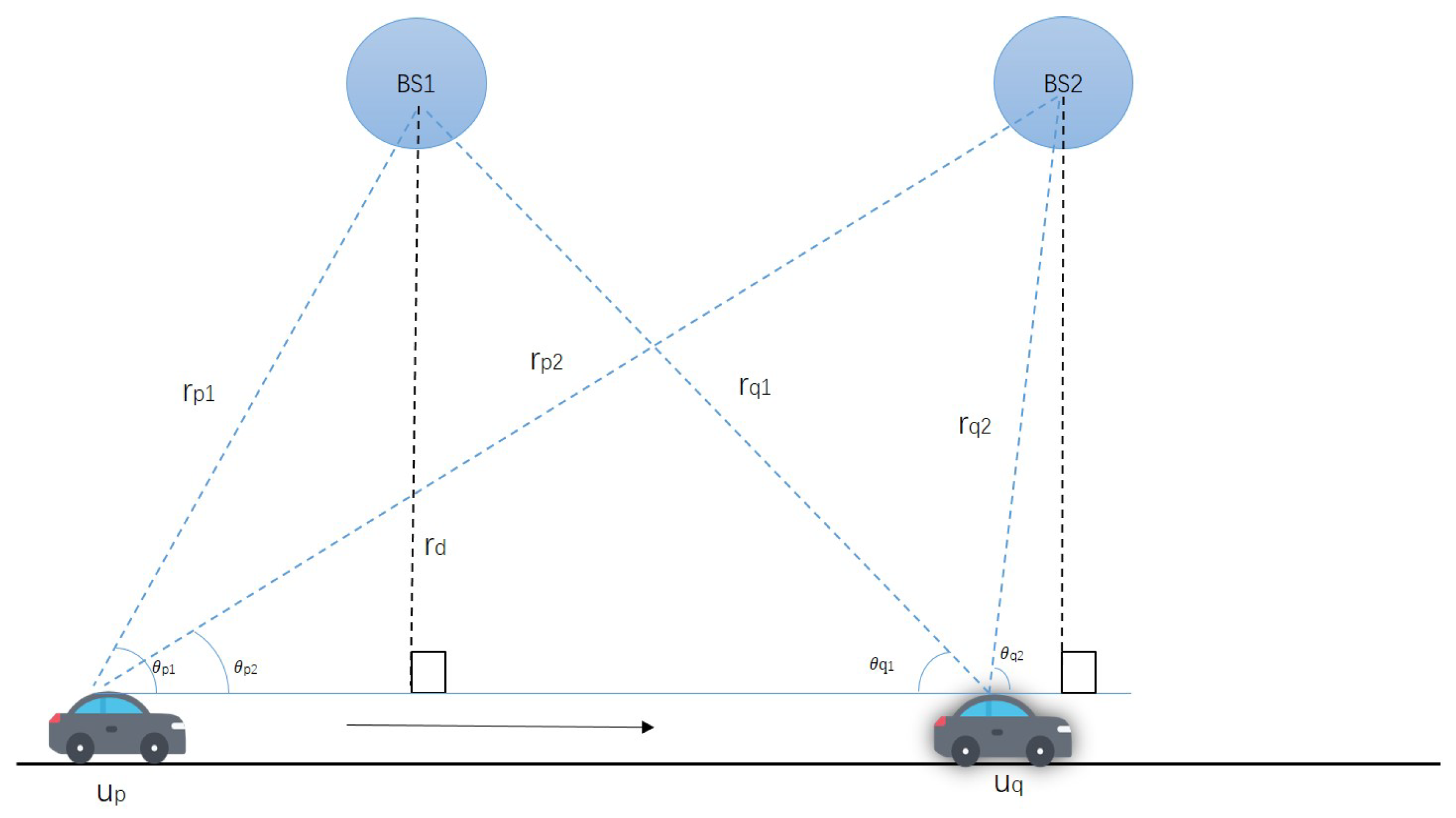
Different variations of geometric distances in Equation (4) have varying effects on the accuracy of the solution. Figure 1 shows the impact of changes in geometric diversity on ambiguity.

As shown in Figure 1, assume that the receiver moves from position p to point q. Base station 1 and base station 2 are at the same height. The carrier phase can be expressed as:

$$\left\{\begin{array}{c}{\varphi }_p^1={\lambda }^{-1}\left(∥{\mathbf{s}}^{\mathbf{1}}-{\mathbf{u}}_{\mathbf{p}}∥+c\delta t_{u_p}-c\delta t^1+c{\tau }_{u_p}+c{\tau }^1\right)+N^1+w_p^1\hfill \\ {\varphi }_p^2={\lambda }^{-1}\left(∥{\mathbf{s}}^{\mathbf{2}}-{\mathbf{u}}_{\mathbf{p}}∥+c\delta t_{u_p}-c\delta t^2+c{\tau }_{u_p}+c{\tau }^2\right)+N^2+w_p^2\hfill \end{array}\right.$$

(5)

where Z denotes AR and $\lambda$ denotes wavelength, w denotes the noise term. The difference between the two equations gives:

$$\begin{array}{cc}\hfill {\varphi }_p^{12}+w_p^{21}& =\frac{r_{p_1}-r_{p_2}}{\lambda }+Z^{12}\hfill \\ \hfill & =\frac{1}{\lambda }·r_d\left(\frac{1}{sin{\theta }_{p_1}}-\frac{1}{sin{\theta }_{p_2}}\right)+Z^{12}\hfill \end{array}$$

(6)

Let $\left(\frac{1}{sin{\theta }_{p_1}}-\frac{1}{sin{\theta }_{p_2}}\right)$ equal to $A_p$. Similarly, based on the above analysis, the following relationship can be obtained at point q:

$$\begin{array}{cc}\hfill & {\varphi }_p^{12}+w_p^{21}=\frac{r_d}{\lambda }{A}_p+Z^{12}\hfill \\ \hfill & {\varphi }_q^{12}+w_q^{21}=\frac{r_d}{\lambda }{A}_q+Z^{12}\hfill \end{array}$$

(7)

$$\left[\begin{array}{c}{\varphi }_p^{12}+w_p^{21}\\ {\varphi }_q^{12}+w_q^{21}\end{array}\right]=\left[\begin{array}{cc}{A}_p& 1\\ A_q& 1\end{array}\right]\left[\begin{array}{c}{\lambda }^{-1}{r}_d\\ Z^{12}\end{array}\right]$$

(8)

The solution of AR can be deduced as:

$$\left[\begin{array}{c}{\lambda }^{-1}{r}_d\\ Z^{12}\end{array}\right]=\frac{1}{A_p-A_q}\left[\begin{array}{cc}1& -1\\ -A_q& A_P\end{array}\right]\left[\begin{array}{c}{\varphi }_p^{12}+w_p^{21}\\ {\varphi }_q^{12}+w_q^{21}\end{array}\right]$$

(9)

When the movement of the receiver has a small displacement, the value of the angular change is minimal, which also means that $A_q$ and $A_p$ are almost equal. In this case, there is the linear correlation of the matrix in Equation (8). Even if the noise term is small, huge errors would be introduced in the positioning, resulting in an erroneous AR solution. Therefore, geometric changes have an impact on AR.

2.3. Linearization of the Model

It can be seen from Equation (4) that when the value of $Z^{ij}$ is obtained, the received carrier phase difference value can be used to calculate the position of the receiver. At the kth epoch, the differenced geometric range can be defined as:

$$\begin{array}{cc}\hfill \Delta r_k^{ij}=& ∥{\mathbf{s}}^i-{\mathbf{u}}_{\mathbf{k}}∥-∥{\mathbf{s}}^j-{\mathbf{u}}_{\mathbf{k}}∥\hfill \\ \hfill =& \sqrt{{\left(x_u^k-x^i\right)}^2+{\left(y_u^k-y^i\right)}^2+{\left(z_u^k-z^i\right)}^2}\hfill \\ \hfill -& \sqrt{{\left(x_u^k-x^j\right)}^2+{\left(y_u^k-y^j\right)}^2+{\left(z_u^k-z^j\right)}^2}\hfill \end{array}$$

(10)

Taking the initial receiver location as ($x_0$, $y_0$, $z_0$), the Taylor series of (10) is expanded to the first-order term as [19]:

$$\Delta r_k^{ij}=\Delta r_0^{ij}+{\left.\frac{\partial \Delta r_k^{ij}}{\partial x_u}\right|}_{x_0}\left(x_u^k-x_0\right)+{\left.\frac{\partial \Delta r_k^{ij}}{\partial y_u}\right|}_{y_0}\left(y_u^k-y_0\right)+{\left.\frac{\partial \Delta r_k^{ij}}{\partial z_u}\right|}_{z_0}\left(z_u^k-z_0\right)$$

(11)

Suppose the total number of base stations is M + 1, the epoch’s unknown coordinate is k and the reference base station is j. Then, The eth iteration loop of the system can be expressed as:

$${\mathit{\rho }}^k\left(e\right)={\mathbf{H}}_A^k\left(e\right){\mathbf{x}}_A^n\left(e\right)+{\mathbf{H}}_B^k{\mathbf{Z}}_B+{\mathit{\omega }}^k$$

(12)

It is important to note that Equation (12) is derived from Equation (4). e is the iteration index.

$${\mathit{\rho }}^k\left(e\right)=\left[\begin{array}{c}\lambda {\varphi }_k^{1j}-\Delta r_k^{1j}(e-1)\\ \lambda {\varphi }_k^{2j}-\Delta r_k^{2j}(e-1)\\ ⋮\\ \lambda {\varphi }_k^{Mj}-\Delta r_k^{Mj}(e-1)\end{array}\right]$$

(13)

$${\mathbf{H}}_A^k\left(e\right)=\left[\begin{array}{ccc}{\left.\frac{\partial \Delta r_k^{1j}}{\partial x_u^k}\right|}_{{\widehat{x}}_u^k(e-1)}\hfill & {\left.\frac{\partial \Delta r_k^{1j}}{\partial y_u^k}\right|}_{{\widehat{y}}_u^k(e-1)}\hfill & {\left.\frac{\partial \Delta r_k^{1j}}{\partial z_u^k}\right|}_{{\widehat{z}}_u^k(e-1)}\hfill \\ {\left.\frac{\partial \Delta r_k^{2j}}{\partial x_u^k}\right|}_{{\widehat{x}}_u^k(e-1)}\hfill & {\left.\frac{\partial \Delta r_k^{2j}}{\partial y_u^k}\right|}_{{\widehat{y}}_u^k(e-1)}\hfill & {\left.\frac{\partial \Delta r_k^{2j}}{\partial z_u^k}\right|}_{{\widehat{z}}_u^k(e-1)}\hfill \\ {\left.\frac{\partial \Delta r_k^{Mj}}{\partial x_u^k}\right|}_{{\widehat{x}}_u^k(e-1)}\hfill & {\left.\frac{\partial \Delta r_k^{Mj}}{\partial y_u^k}\right|}_{{\widehat{y}}_u^k(e-1)}\hfill & {\left.\frac{\partial \Delta r_k^{Mj}}{\partial z_u^k}\right|}_{{\widehat{z}}_u^k(e-1)}\hfill \end{array}\right]$$

(14)

$${\mathbf{x}}_A^k\left(e\right)={\left[\left(x_u^k-{\widehat{x}}_u^k(e-1)\right)\left(y_u^k-{\widehat{y}}_u^k(e-1)\right)\left(z_u^k-{\widehat{z}}_u^k(e-1)\right)\right]}^{\mathrm{T}}$$

(15)

$${\mathbf{H}}_B^k=\lambda {\mathbf{I}}_{M\times M}$$

(16)

$${\mathbf{Z}}_B={\left[\begin{array}{cccc}{Z}^{1j}\hfill & Z^{2j}\hfill & \cdots \hfill & Z\hfill \end{array}\right]}^{\mathrm{T}}$$

(17)

The covariance matrix of the noise $\omega$ is described as:

$${\mathbf{R}}_{\rho }\left(m\right)=\left[\begin{array}{cccc}{\sigma }_{\Delta \varphi }^2& \frac{{\sigma }_{\Delta \varphi }^2}{2}& \cdots & \frac{{\sigma }_{\Delta \varphi }^2}{2}\\ \frac{{\sigma }_{\Delta \varphi }^2}{2}& {\sigma }_{\Delta \varphi }^2& \cdots & \frac{{\sigma }_{\Delta \varphi }^2}{2}\\ ⋮& ⋮& \ddots & ⋮\\ \frac{{\sigma }_{\Delta \varphi }^2}{2}& \frac{{\sigma }_{\Delta \varphi }^2}{2}& \cdots & {\sigma }_{\Delta \varphi }^2\end{array}\right]$$

(18)

When selecting data of several epochs:

$$\mathit{\rho }={\mathbf{H}}_A{\mathbf{x}}_A+{\mathbf{H}}_B{\mathbf{Z}}_B+\omega$$

(19)

$$\mathit{\rho }={\left[\begin{array}{cccc}{\mathit{\rho }}^1\hfill & \cdots \hfill & {\mathit{\rho }}^k\hfill & \cdots \hfill \end{array}\right]}^{\mathrm{T}}$$

(20)

$${\mathbf{x}}_A={\left[\begin{array}{cccc}{\mathbf{x}}_A^1\hfill & \cdots \hfill & {\mathbf{x}}_A^k\hfill & \cdots \hfill \end{array}\right]}^{\mathrm{T}}$$

(21)

$${\mathbf{H}}_A=\left[\begin{array}{cccc}{\mathbf{H}}_A^1& & & \\ & \ddots & & \\ & & {\mathbf{H}}_A^k& \\ & & & \ddots \end{array}\right],{\mathbf{H}}_B=\left[\begin{array}{c}{\mathbf{H}}_B^1\\ ⋮\\ {\mathbf{H}}_B^k\\ ⋮\end{array}\right]$$

(22)

Equation (19) can be solved using the least squares method.

2.4. Linearization Error and Solution Analysis

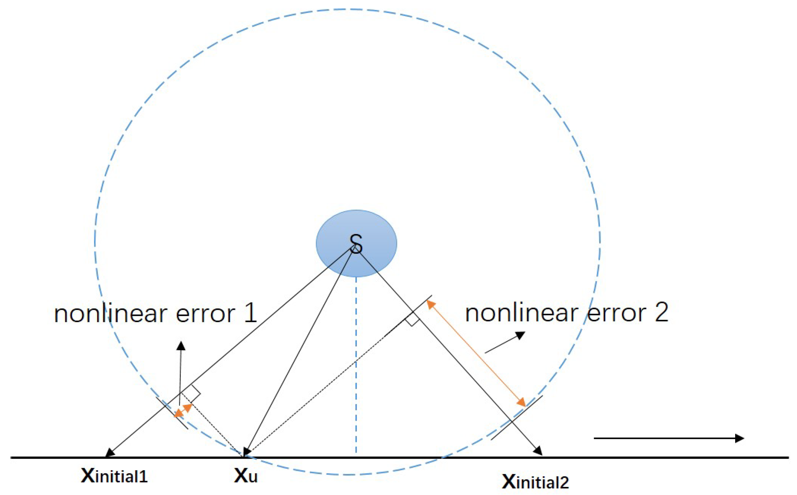
Though it is possible to linearize the model by Taylor expansion and then use the least-squares method to find the estimator. The linearization error depends on the function’s degree of nonlinearity and how far from the working point the linear approximation is used. Therefore there are limitations. The linearization error is small when the initial position deviation is slight, as shown in Figure 2.

Moreover, the algorithm can converge in point $x_{initial1}$. If the initial deviation is significant, as in the case of scenario $x_{initial2}$, the linearization error is significant. When Jacobi Matrix does not have an inverse matrix, the solution cannot be obtained using the least square method.

The ground-based position system dynamics are highly nonlinear. Furthermore, there are many cases where the Jacobian cannot be found analytically. Since the uncertainty of the unknown value of the AR is substantial, its range cannot be limited, and the search method cannot find the initial value. In some existing methods, several known points are used for solving AR, which would cause inconvenience to the solution. In the next part of this paper, we introduce the proposed new model, which does not require the aid of known points.

3. The Proposed Method of the Robotic System

In this section, the proposed model is introduced, which eliminates ambiguity. After that, the swarm intelligence optimization algorithm can be used to find the close initial point coordinates.

3.1. A-OTF Model

We propose the A-OTF model is a double difference ground-base model. It should be emphasized that this model is different from the double-difference model of the RTK positioning method commonly used in GNSS. In the RTK positioning method, two receivers called base and rover are needed. The A-OTF model uses only one receiver, uses the difference between base stations to eliminate clock drift effects, and then uses the re-differentiation between the duration epochs to eliminate ambiguity. Subtracting the single difference between the two epochs:

$$\begin{array}{cc}\hfill {\varphi }_{k,k+1}^{ij}-w_{k,k+1}^{ij}& ={\lambda }^{-1}\left(∥{\mathbf{s}}^i-{\mathbf{u}}_k∥-∥{\mathbf{s}}^j-{\mathbf{u}}_k∥-∥{\mathbf{s}}^i-{\mathbf{u}}_{k+1}∥+∥{\mathbf{s}}^j-{\mathbf{u}}_{k+1}∥\right)\hfill \\ \hfill & ={\lambda }^{-1}\left(\Delta r_k^{ij}-\Delta r_{k+1}^{ij}\right)\hfill \end{array}$$

(23)

${\varphi }_{k,k+1}^{ij}$ is the difference of the selected single differential carrier phase from Equation (4). k and k + 1 denote the two epochs selected for the AR solution.

For each additional epoch, the number of unknowns increases by 3 (x, y, z), and the number of equations increases by M (M + 1 is the total number of base stations). Due to the initial position, the equation can be solved when the epoch satisfies the following relation: $M\ast (n-1)>3\ast n$ (n denotes the number of epochs). If ith base station is the reference base station. Then, the system of equations can be listed as:

$$\left\{\begin{array}{cc}{\varphi }_{k,k+1}^{ij}-w_{k,k+1}^{ij}& ={\lambda }^{-1}\left(\Delta r_k^{ij}-\Delta r_{k+1}^{ij}\right)\\ {\varphi }_{k,k+1}^{ie}-w_{k,k+1}^{ie}& ={\lambda }^{-1}\left(\Delta r_k^{ie}-\Delta r_{k+1}^{ie}\right)\\ \dots & \dots \\ {\varphi }_{k,k+1}^{iM}-w_{k,k+1}^{iM}& ={\lambda }^{-1}\left(\Delta r_k^{iM}-\Delta r_{k+1}^{iM}\right)\\ ⋮& ⋮\\ {\varphi }_{k,k+n}^{ij}-w_{k,k+n}^{ij}& ={\lambda }^{-1}\left(\Delta r_k^{ij}-\Delta r_{k+n}^{ij}\right)\\ {\varphi }_{k,k+n}^{ie}-w_{k,k+n}^{ie}& ={\lambda }^{-1}\left(\Delta r_k^{ie}-\Delta r_{k+n}^{ie}\right)\\ {\varphi }_{k,k+n}^{iM}-w_{k,k+n}^{iM}& ={\lambda }^{-1}\left(\Delta r_k^{iM}-\Delta r_{k+n}^{iM}\right)\end{array}\right.$$

(24)

There are no ambiguity and clock difference values in Equation (24). Only the positions of the coordinate are unknowns. Since the localization range is known, the search space can be restricted according to the localization range, and the approximate solution could be searched by using the intelligent swarm algorithm.

3.2. The Initial Solution Using Adaptive Particle Swarm Algorithm

A term in the Equation (24) can be simplified as follows:

$$loss={[{\varphi }_{k,k+l}^{ij}-{\lambda }^{-1}\left(\Delta r_k^{ij}-\Delta r_{k+l}^{ij}\right)]}^2$$

(25)

The search objective of the nonlinear intelligence algorithm is to find the coordinate points u1, u2, un to minimize the value of F.

$$fitness=\underset{\mathbf{u}\mathbf{1},\mathbf{u}\mathbf{2},\dots }{argmin}\sum _{l=1}^n\sum _{j=2}^M{[{\underset{\mathbf{R}}{\varphi }}_{k,k+l}^{ij}-{\lambda }^{-1}\left(\Delta r_k^{ij}-\Delta r_{k+l}^{ij}\right)]}^2$$

(26)

where $\mathbf{R}=E\left[\mathbf{w}{\mathbf{w}}^{\mathbf{T}}\right]$ represents the noise covariance matrix. The adaptive PSO algorithm is used for finding the optimal solution that represents the fitness of the loss function. It is a stochastic algorithm of optimization based on swarm intelligence. The search space of the problem is compared with the flight space of a bird. It simulates the foraging behavior of birds and denotes the candidates for problem solving by abstracting each bird as a particle. The method is applicable to nonlinear optimization problems of ground-based navigation systems. The PSO algorithm requires a given range of search spaces. Based on this, a set of parameter values is searched in the loop iteration to minimize the fitness value.

The particle population consists of D particles forming the population:

$$X=\left(X_1,X_2\cdots X_D\right)$$

(27)

Each particle is a set of candidate solutions:

$${\mathrm{X}}_i={\left(x_u^1,y_u^1,z_u^1\dots ,x_u^n,x_u^n,x_u^n\right)}^{\top }$$

(28)

The speed is:

$$V_i={\left(v_x^1,v_y^1,v_z^1,\cdots ,v_z^n\right)}^T$$

(29)

In the t + 1 iteration, the speed is updated as:

$$V_i^{k+1}=V_i^k+c_1{r}_1\left(P_i^k-X_i^k\right)+c_2{r}_2\left(P_g^k-X_i^k\right)$$

(30)

where $P_i^k$ and $P_g^k$ denote the extreme individual value and the global optimum, respectively. $c1$, $c2$, and $r1$, $r2$ are parameters that need to be set in advance. r1, r2 are random numbers between [0,1]. $c1$ and $c2$ are called learning factors. The location is updated as:

$$X_i^{k+1}=X_i^k+V_i^{k+1}$$

(31)

The update of the position can be limited according to the positioning area of the receiver. Ground-based positioning is a highly nonlinear optimization problem, and the PSO algorithm has good optimization capabilities. Through iterative optimization calculations, approximate solutions can be found quickly. However, the basic PSO algorithm can easily fall into a local optimum, which leads to significant errors. It can be seen from the position update model in Equation (30), The degree of particle velocity update determines how fast the global convergence of the algorithm is achieved. When the speed is very high, the optimal solution is easily crossed due to ineffective control. When the speed is low, the global search capability of the algorithm decreases. In this paper, we adopt the PSO algorithm with adaptive weights adjustment. The speed is updated as:

$$V_i^{k+1}=\omega V_i^k+c_1{r}_1\left(P_i^k-X_i^k\right)+c_2{r}_2\left(P_g^k-X_i^k\right)$$

(32)

where $\omega$ is denoted as the nonlinear dynamic inertia weight coefficient, and the update process is:

$$\omega =\left\{\begin{array}{c}{\omega }_{min}-\frac{\left({\omega }_{max}-{\omega }_{min}\right)\ast \left(\mathit{fitness}-{\mathit{fitness}}_{min}\right)}{{\mathit{fitness}}_{\mathrm{avg}}-{\mathit{fitness}}_{min}},\mathit{fitness}⩽{\mathit{fitness}}_{\mathrm{avg}}\hfill \\ \\ {\omega }_{max},\mathit{fitness}>{\mathit{fitness}}_{\mathrm{avg}}\hfill \end{array}\right.$$

(33)

Among them, ${\omega }_{max}$ and ${\omega }_{min}$ are the initial values set in advance, which are 0.8 and 0.5 in this paper, respectively. ${\mathit{fitness}}_{\mathrm{avg}}$ and ${\mathit{fitness}}_{\min }$ are the average target value and minimum value of the particles.

When the current particle value obtained by calculation is better than the average value, Equation (34) can be used to reduce its weighting factor to retain the particle. On the contrary, the weight factor is increased to allow the particles to have a higher speed and move closer to the area with a smaller fitness value.

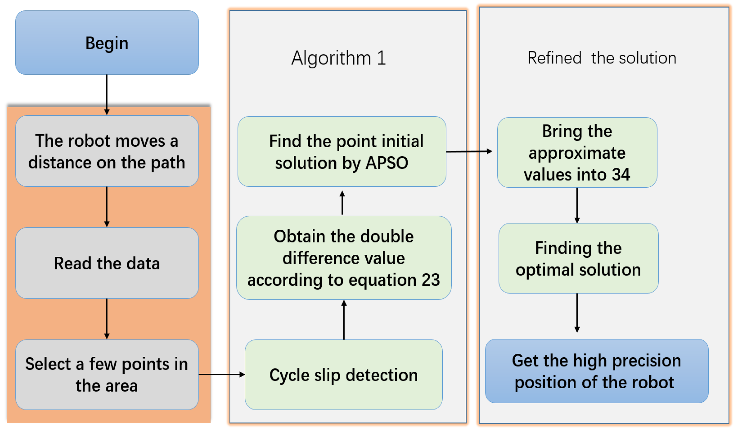
The process of finding the initial solution of the ground-based Robotic system by the adaptive PSO is shown in Algorithm 1.

3.3. Refined Solution and the Flow of the Algorithm

When the initial approximate solution of the position is obtained, it can be used to solve the high-precision value of the ambiguity.

$$\widehat{{\mathbf{z}}_B}=\underset{{\mathbf{x}}_{\mathrm{initial}}}{argmin}{∥{\mathbf{H}}_A{\mathbf{x}}_A+{\mathbf{H}}_B{\mathbf{Z}}_B-\mathit{\rho }∥}_{\mathbf{R}}$$

(34)

After obtaining the ambiguity value, the high-precision positioning position can be found according to the carrier phase values. The flow chart of the robot positioning procedure is presented in Figure 3.

Algorithm 1 Adaptive Particle Swarm Algorithm.

Require: Each particle’s optimal global position of the particle population is set as $p_b$ and the current historical optimal position is set as $cu{r}_b$. Ensure: The velocity and position of each individual in the group are initialized according to the number of selected coordinate points (n). The search space dimensions are $3\ast n$. Set the scope of the space according to the positioning area. 1: Set the loop termination condition. When the average particle distance from the actual position is less than 0.2 m, stop the optimization. The maximum amount of iteration is 100. 2: The fitness value for each individual particle is evaluated according to Equation (26). Store the $cu{r}_b$ and fitness values and select the optimal value from the population. 3: The velocity and position of the particles are updated based on Equations (31) and (32). 4: Calculate the updated fitness value and compare it with $cu{r}_b$. If it is lower than $cu{r}_b$, then update c. Similarly, compare the value with $p_b$. 5: If the value of $p_b$ meets the termination condition or the iteration loop has reached the upper limit, terminate the loop, otherwise continue to step 2. 6: return$fitness$ and the $p_b$;

It is worth noting that the value of ambiguity does not change if no signal loss lock or cycle slips occurs. The cycle slips have a great influence on the positioning result, even if it occurs one cycle, there would be an error of nearly 20 cm. Fortunately, cycle slips can be detected with high sensitivity using the model proposed in this paper. Related content is introduced in the actual system verification section.

4. Simulation Tests

In this section, simulations with different trajectories are carried out to find the effect of different trajectories on the accuracy of the solution. The signal carrier frequency is set to 1575.42 MHz, and the carrier wavelength is approximately 19.08 cm. It is assumed that the standard deviation (STD) of the measured noise is 0.01 to 0.05 cycles based on several previous studies [21,25].

4.1. Simulation Scenario Setting

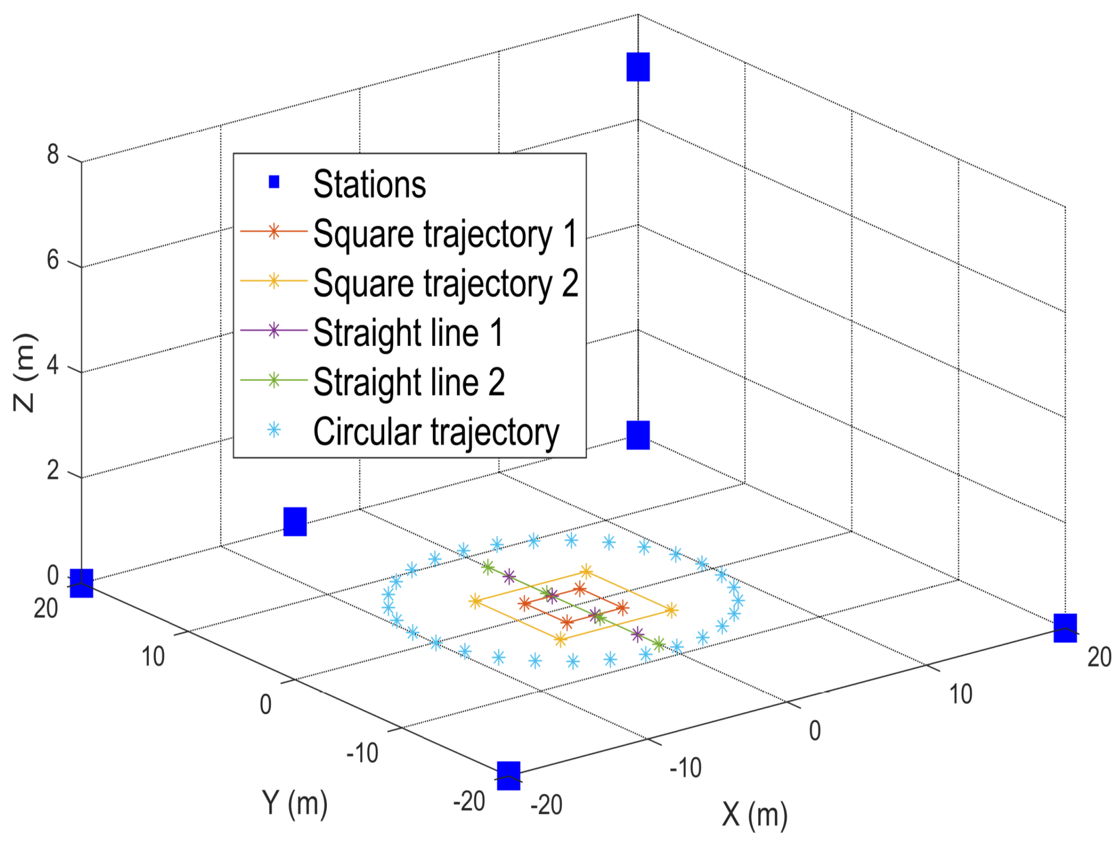
As shown in Figure 4, six base stations are used in the simulation scenario to be arranged in different positions in a 20 m × 20 m × 8 m space.

The coordinates of the transmitting antenna are shown in

Table 1. Coordinates of transmitter antennae.

Station	X (m)	Y (m)	Z (m)
BS1	−20	−20	0
BS2	20	−20	0
BS3	20	20	0
BS4	−20	20	0
BS5	20	20	7
BS6	−20	0	3

.

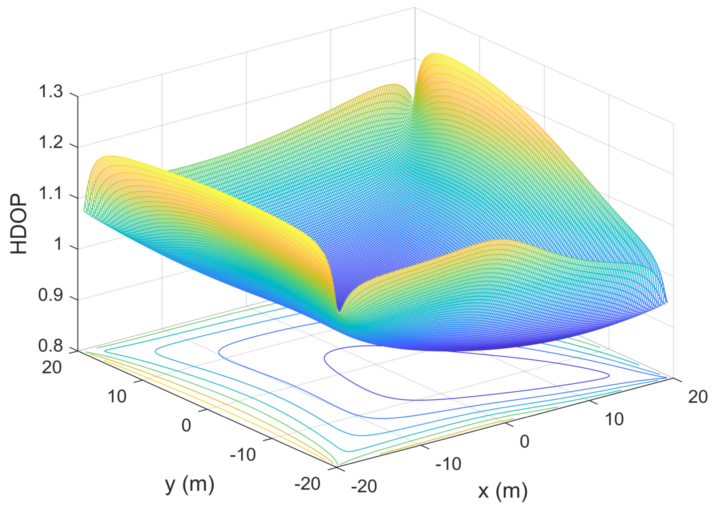
There are different geometric accuracy factors at various locations in the simulation scene due to the change in angle corresponding to the stations. The calculation of the horizontal dilution of precision (HDOP) is as follows [26,27]:

$$\mathrm{HDOP}=\sqrt{{\tilde{h}}_{11}+{\tilde{h}}_{22}}$$

(35)

The accuracy factor for the vertical dilution of precision (VDOP) is calculated as:

$$\mathrm{VDOP}=\sqrt{{\tilde{h}}_{33}}$$

(36)

$\tilde{h}$ represents the diagonal elements of the weight coefficient matrix.

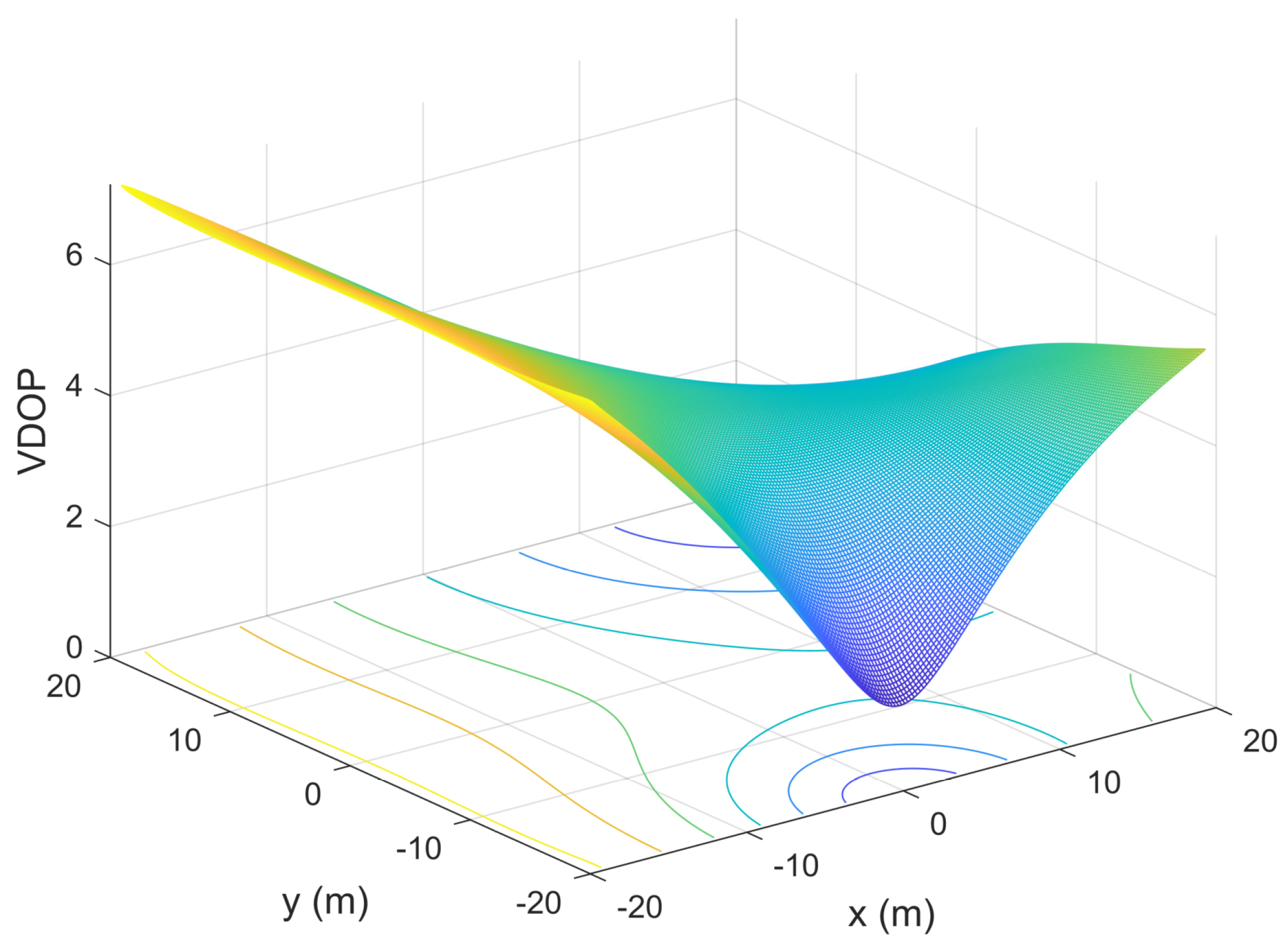
The distribution of the dilution of precision in the scenario is shown in Figure 5 and Figure 6. Since more attention is focused on horizontal accuracy in real-world positioning, and the altitude direction is almost constant. The geometric factors in the horizontal direction are evenly distributed, and the difference between the distribution values is slight, between 1 and 1.3. While in vertical height, the value of VDOP varies drastically due to the slight variation in relative height between the base stations.

4.2. Simulation Results of Different Trajectory Scale

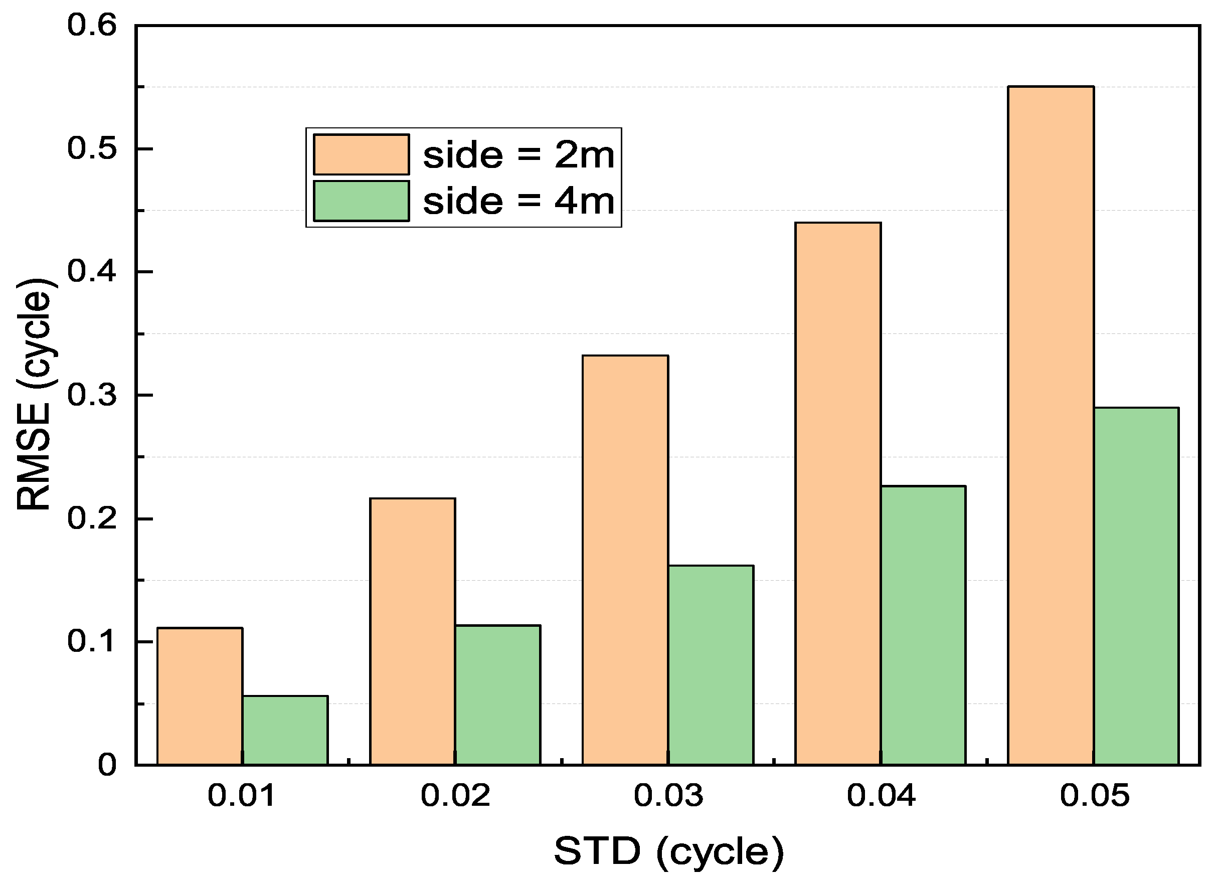
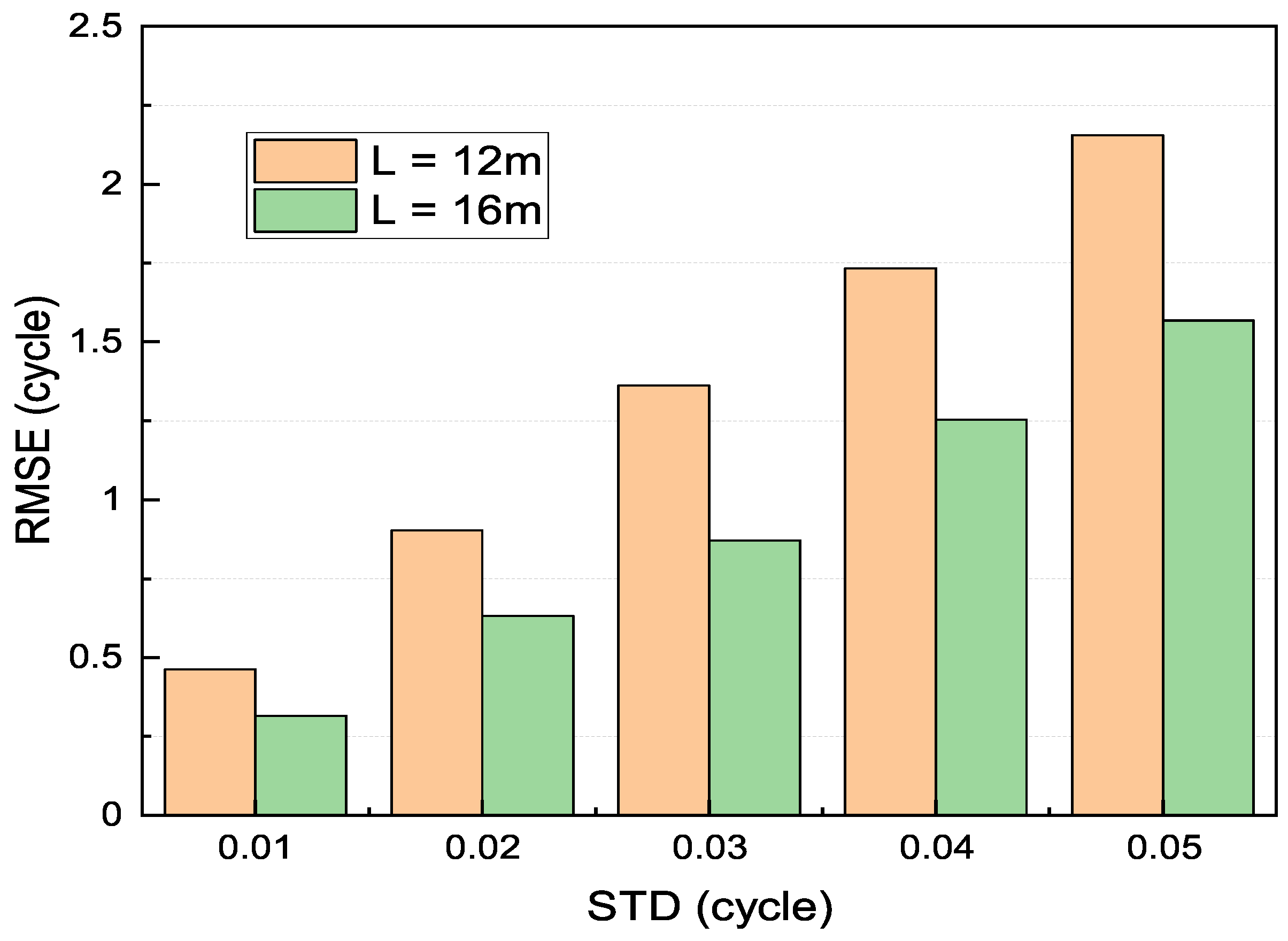
In order to verify the effect of sizing on positioning accuracy, simulations of different scales of square and straight lines are performed experimentally.

As shown in Figure 7 and Figure 8, the number of points taken is four, and the accuracy of the AR solution is improved when the moving distance increases. In this scenario, the AR accuracy is better than 0.3 cycles for different standard deviations when solving with four vertices of a square with a side length of 4 m.

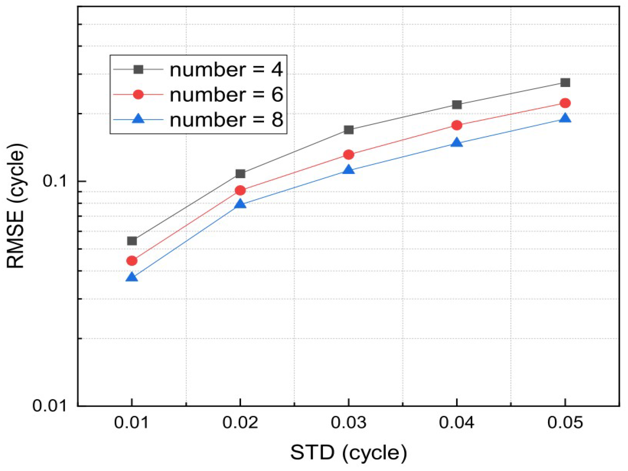
4.3. Simulation Results of Different Points of the Trajectory

In this section, a circular trajectory with a radius of 6 m was used. Four, six, and eight points were selected at equal intervals for simulation experiments. The result is shown in Figure 9.

As the number of points increases, the accuracy of the solution increases accordingly, as shown in Figure 9. However, the amount of calculation will increase. Therefore, the number of selected points should be treated differently according to different application scenarios.

5. Real-World Experiments in Robot Systems

In this section, we conducted a real-world experiment in robot system to verify the accuracy of the positioning results and the AR in practice.

5.1. Experimental Equipment and Scenario

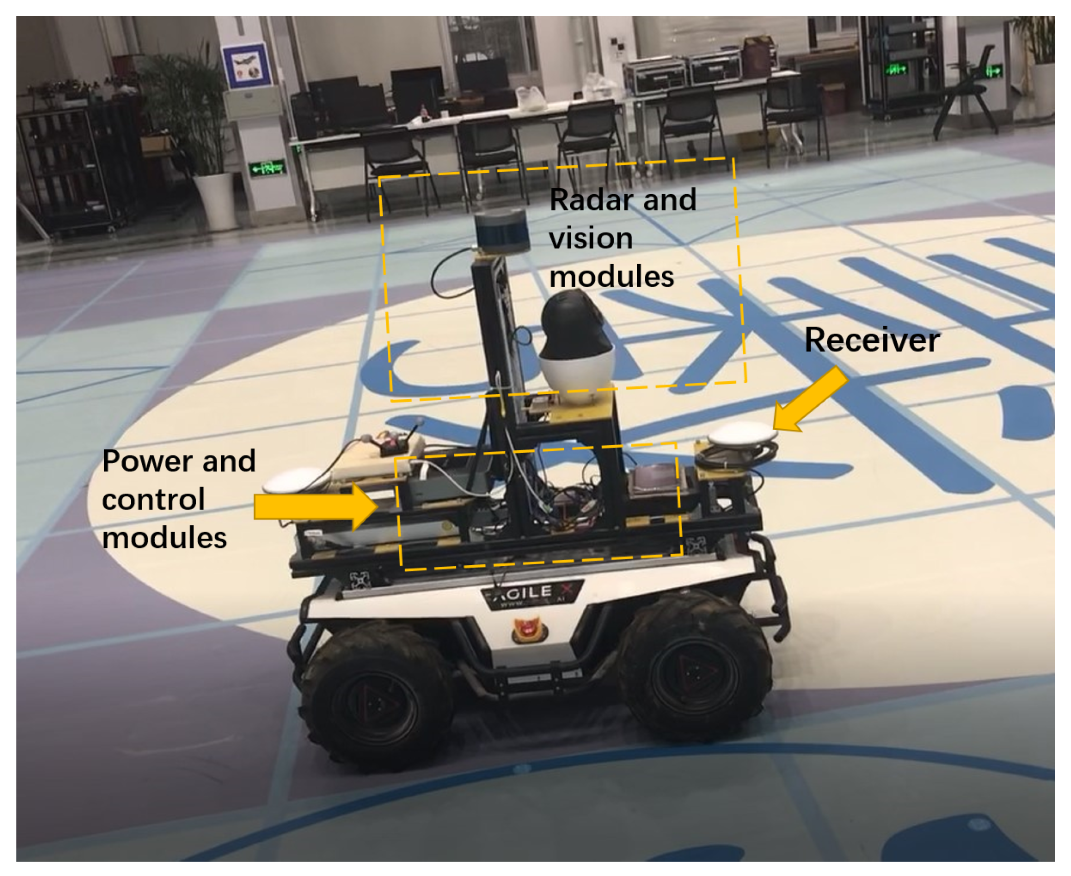
A multi-sensor fusion wheeled cart is used for the experiment. It mainly contains the radar, power and control modules and the receiver module for experimental verification, as shown in Figure 10.

The receiver contains the receiving antenna and the data processing module. The positions of the sensors have been calibrated. The sampling frequency of the receiver is 5 Hz.

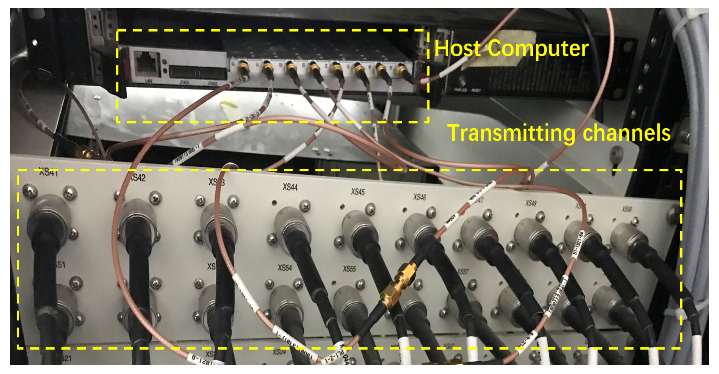
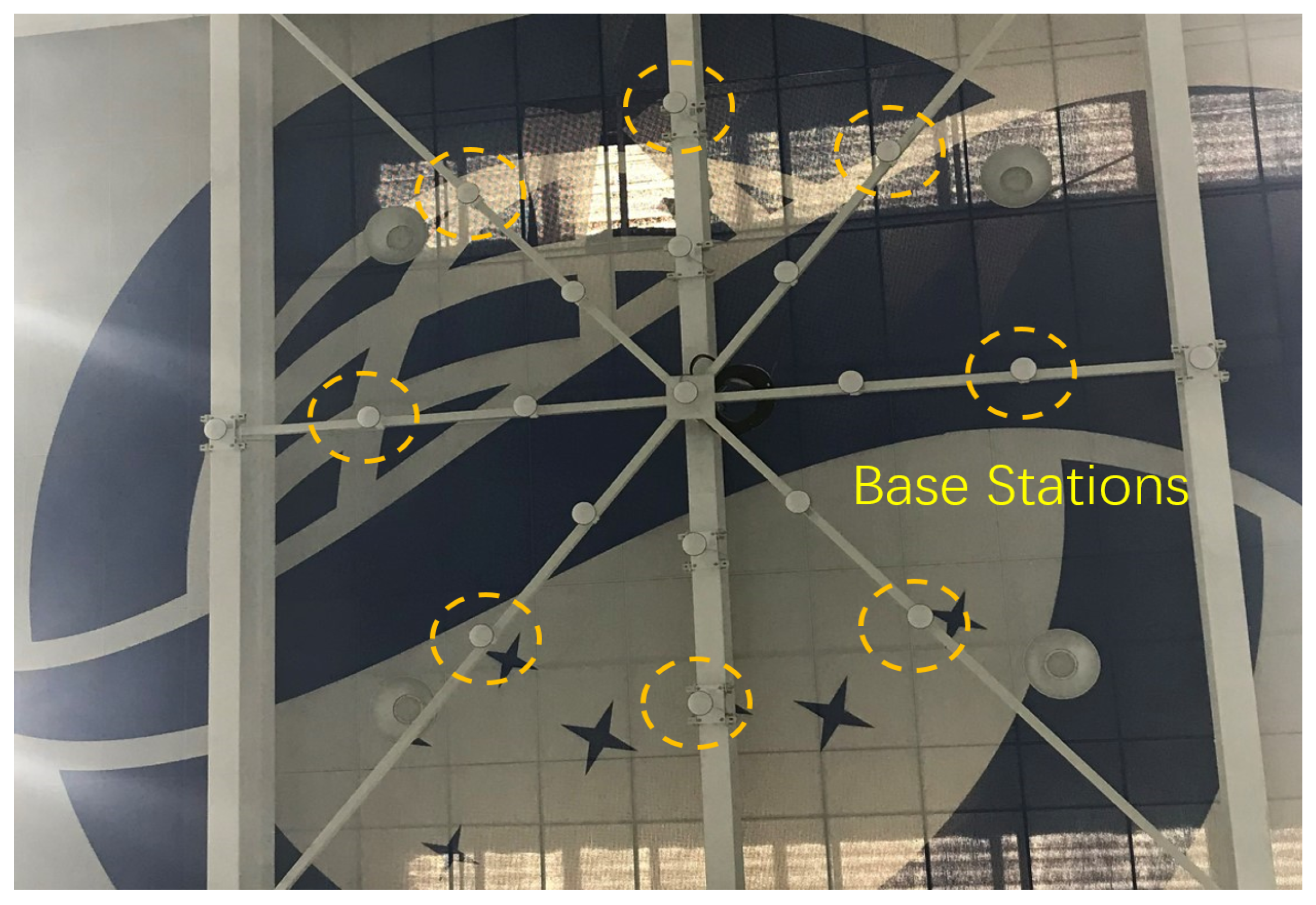
The transmitting antennas representing the base stations are connected by wires to maintain frequency synchronization. The control host computer and the transmitting channels are shown in Figure 11. The signal carrier frequency is 1575.42 MHz. Eight base stations are evenly distributed on the same horizontal plane, as shown in Figure 12.

The base station is deployed on the roof, and the coordinates are shown in

Table 2. Antenna Array Coordinates.

Base Stations	X (m)	Y (m)	Z (m)
BS1	1.412	2.809	11.344
BS2	1.980	4.376	11.341
BS3	1.191	5.839	11.337
BS4	−0.148	6.229	11.360
BS5	−1.420	5.664	11.335
BS6	−1.988	4.130	11.493
BS7	−1.239	2.660	11.343
BS8	0.113	2.242	11.365

.

5.2. Cycle Slip Detection Analysis

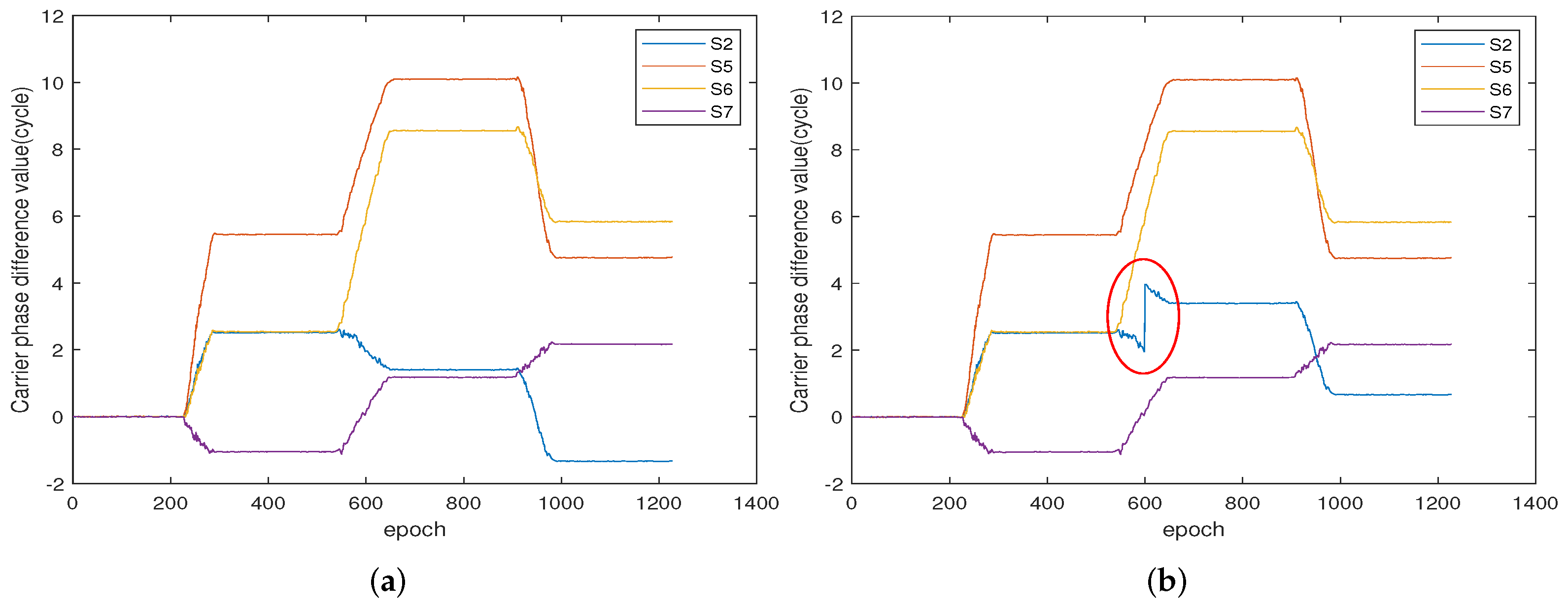
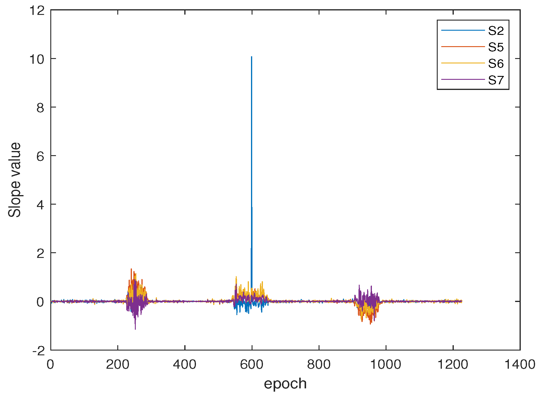
Cycle slip detection belongs to the part of data preprocessing, which ensures the correctness of observations. Similar to GNSS, cycle slips can occur in GBPS and cause interference to carrier phase positioning. Fortunately, our model can detect and correct the cycle slips in time to provide the correct carrier phase data for high-precision positioning, which is also an advantage of the model. We used the real collected linear motion data and added simulated cycle slips for illustration, as shown in Figure 13.

The straight line indicates that the receiver is static, while the oblique line indicates that the receiver is moving in Figure 13a. We add cycle slip at around 600 epochs, with a size of 2 cycles, as shown in Figure 13b. It can be seen from Figure 14 that the station (blue line) where the cycle slip occurs has apparent bumps. We find the slope between the epochs of the received data, as shown in Figure 14.

The slope of the cycle slip about 10 (frequency is 5 Hz, sometimes 10 Hz is used), and the other positions are below 1.5. We can set a threshold equal to 4, to determine whether a cycle slip has occurred. After that, we can repair or discard the data of the station for position solving.

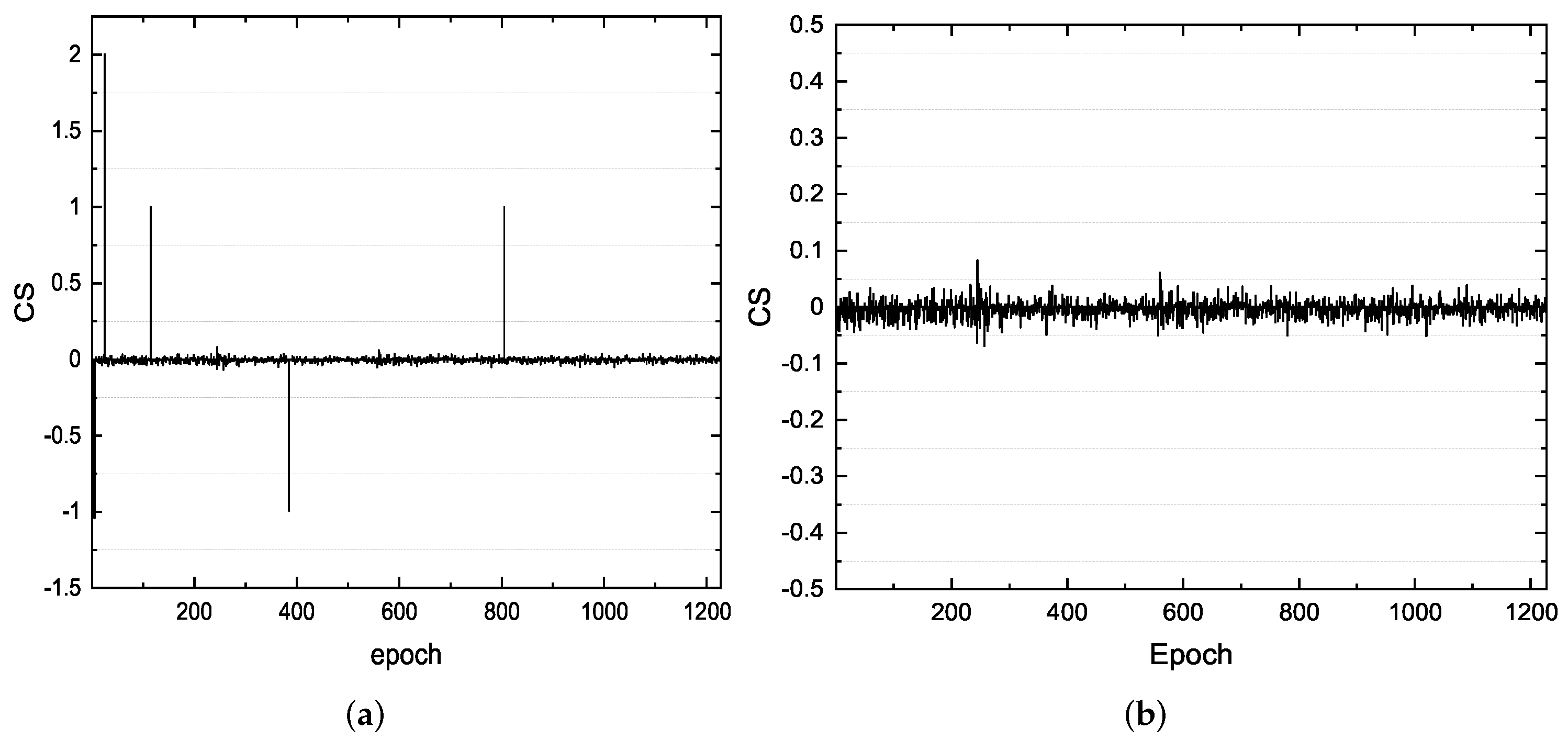
The accuracy of the carrier phase should be guaranteed after a distance movement. When several cycle slips occur, Doppler information can assist in detection and repair:

$$\begin{array}{cc}\hfill & \Delta {\mathsf{\Phi }}_{Li1}={\mathsf{\Phi }}_{Li}\left(t\right)-{\mathsf{\Phi }}_{Li}(t-1)\hfill \\ \hfill & \Delta {\mathsf{\Phi }}_{Li2}=-\left[{\mathrm{D}}_{Li}\left(t\right)+{\mathrm{D}}_{Li}(t-1)\right]dt/2\hfill \\ \hfill & \mathrm{CS}=\left(\Delta {\mathsf{\Phi }}_{Li1}-\Delta {\mathsf{\Phi }}_{Li2}\right)\hfill \end{array}$$

(37)

where CS is the number of cycle slips, CS is close to 0 when there is no cycle slip. $\mathsf{\Phi }$ denotes the carrier phase data, and $\mathrm{D}$ denotes Doppler information. dt denotes the sampling interval. We added four different numbers of circumferential hops in the S3 carrier phase of the moving receiver, and the results of cycle slip detection and repair are shown in Figure 15.

5.3. Moving Trajectory and Positioning Accuracy

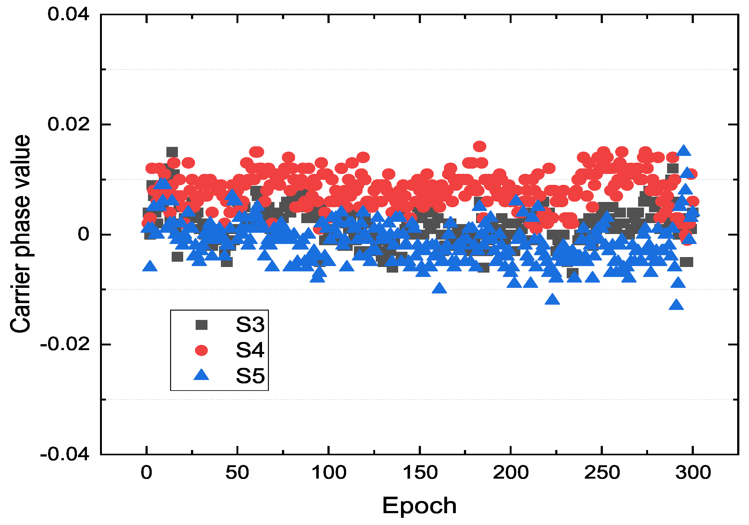
First, we analyzed the noise situation of the carrier phase of the base station. The receiver is stationary for a period of time in the localization area, and the data of 300 epochs are used to analyze the standard deviation of the noise.

The double-differential results for base station three, four, and five at stationary state are shown in Figure 16 (the reference differential station is station one). The average value of the standard deviation of all base stations is 0.0037 cycle, which indicates that the system has centimeter-level positioning capability.

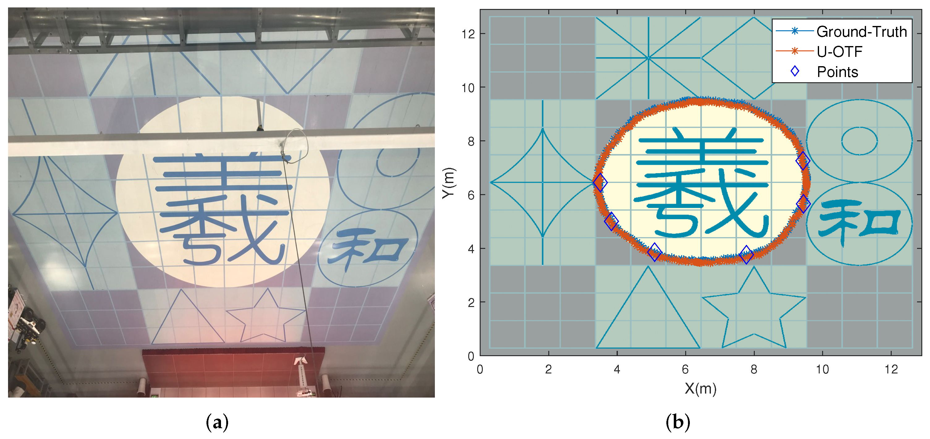
The test area was a 12.5 m × 12.5 m indoor environment of constant height. The path of the multi-sensor cart moved as a circular trajectory in the center of the field.

As the vehicle moves, the resultant value of the double difference of each base station gradually changes from 0.

Six points were evenly selected for the AR as shown in Figure 17. The initial position was found using the particle swarm algorithm (Equation (26)), and the average value of the initial deviation for the six points was calculated to be 0.56 m. Afterward, the optimal solution of AR is performed by using Equation (34). Once the AR is obtained, the location of all epochs can be determined by using the least-squares method. The position of ground truth was determined using a high precision total station. The results of the resolved position are shown in Figure 17.

The vehicle moved in a circle at a smooth speed with a radius of 3 m. The RMSE of the refined solution was about 4.3 cm. This experiment showed that the proposed method can achieve centimeter-level accurate positioning.

6. Discussion

This study shows that A-OTF can achieve high precision positioning with robustness under the condition that system noise statistics involve uncertainty. The proposed double-difference model can provide the search range of solutions for nonlinear intelligent algorithms. It dramatically simplifies the algorithm’s complexity and provides new ways of solving AR for high precision ground-based navigation. It also provides ideas for other strongly nonlinear problems.

Adaptive PSO provides an approximate initial solution for the AR. A-OTF does not use pseudo-range data and can be applied in indoor environments with severe multipath. Unlike the method using known points for initialization, A-OTF does not depent on a priori information. Compared with DDS-OTF (double difference square on the fly), it does not require fitting the receiver’s crystal residuals, which can cause inconveniences. On the other hand, the residual fitting error would cause a significant positioning error when a low stability crystal oscillator is used. Different from DDS-OTF, which requires matrix calculations for dozens of points simultaneously. Only a few points need to be calculated by using A-OTF, which improves the calculation efficiency. In addition, we demonstrated the high sensitivity of the A-OTF method for cycle slip detection by actual measurement data. It ensures the accuracy of the data used for high-precision positioning. However, like the previous methods, the requirement of geometric diversity leads to some limitations of the algorithm.

From the results in the simulation, points with a certain interval distance should be selected to improve the accuracy of AR. The carrier phase double difference results can describe the change in the position of the receiver. These selected points are kept distant from each other in Equation (24) to make a geometric change for the receiver. The increase in precision reduces the real-time performance of the algorithm.

The real-time performance of the algorithm can be improved if other positioning sensors are available. During the AR solution, sensors such as inertial navigation can be used to assist in meeting the continuity of real-time positioning, which is also our future work.

We proved that path scale and diversity have an important influence on AR solutions through theoretical calculations and simulations. The increase of the geometric scale and the path change help improve the AR accuracy. This finding brings guidance to AR solving in GBPS.

7. Conclusions

This paper proposes a novel adaptive AR method to address the classical solutions that rely on initial points or high precision measurement instruments. This paper’s innovation is to establish a double-difference model to remove the base station clock difference and carrier phase ambiguity to obtain the coordinate position approximation initial solution. These points ensure that the initial nonlinear error is within the controllable range during the iteration of the refined stage. The PSO method for finding the initial solution uses an adaptive technology, which can quickly iteratively converge in different noises and paths. This is also the first work in GBPS that considers cycle slip and high-precision AR simultaneously. This method is suitable for scenarios where reliable code measurements are lacking or multipath is severe, allowing base station synchronization inaccuracies and thus making system deployment easier. It can also effectively control the computational load involved in OTF, leading to a significant improvement of computational performance for real-time applications in ground-based systems. In addition, the paper explores the impact of path changes on AR solutions. Real-world experiments verified the reliability of the method.

Future research efforts will focus on the improvement of the proposed A-OTF. It is expected to be combined with artificial intelligence techniques such as neural networks and advanced expert systems to estimate system noise’s statistical properties automatically. In addition, we will verify the system’s reliability using different test scenarios.