
Remaining Useful Life Prediction of Lithium-Ion Batteries Based on Deep Learning and Soft Sensing

Abstract
:1. Introduction
- (1)
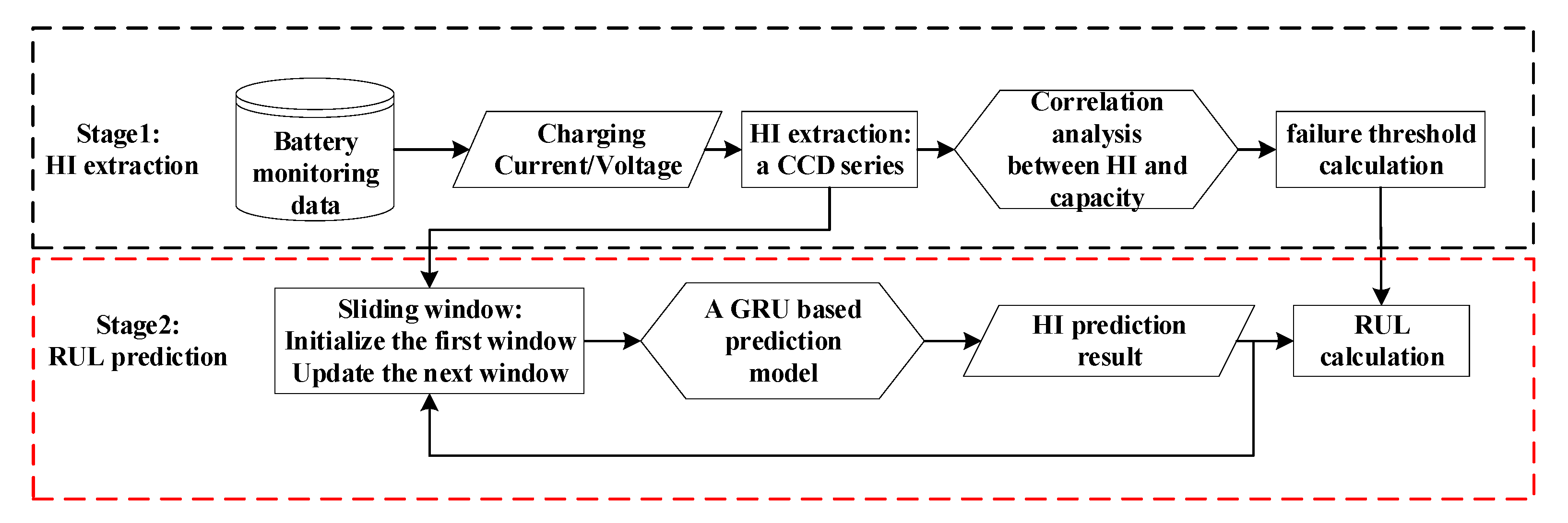
- Combining soft sensing with deep learning, a reliable RUL prediction model is proposed, which can accomplish a satisfactory HI estimation and provide an accurate RUL for LIBs in the routine environment.
- (2)
- A unique indirect HI, i.e., the CCD extracted from the charge monitoring data, is considered as the indirect HI without complicated measurements and time-consuming calculations, providing a soft measurement of battery performance degradation.
- (3)
- A GRU prediction network with an adaptive sliding window is utilized to estimate the HI tendencies and determine the battery residual life. The designed GRU NN can not only learn the long-term dependencies but also fit the local regenerations and fluctuations of the battery degeneration with low computation cost.
2. HI Extraction
2.1. Test Data
2.2. HI Extraction
3. Algorithm Description
3.1. GRU Prediction with Adaptive Sliding Window
- (1)
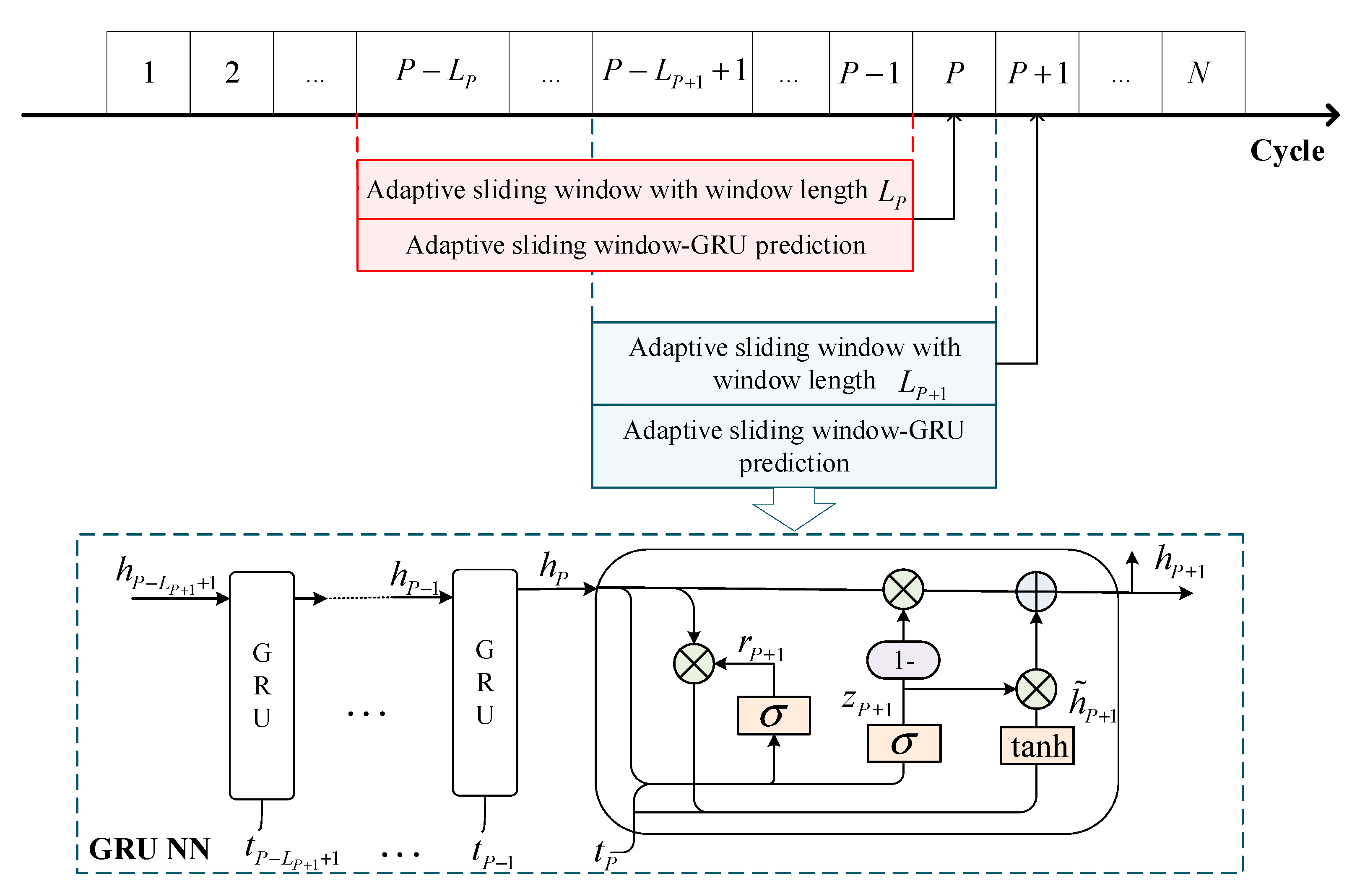
- The sliding mode of the window is set as one-step ahead, i.e., the number of the new data in the window adds only one for each step. Let the current point be P, and the next point be P + 1; the value of the CCD at P + 1 needs to be predicted.
- (2)
- In the online training stage, through selecting the initial window length and performing the one-step-ahead prediction, the CCD data for training are expanded into two-dimensional space to explore the structure and parameters of the GRU NN. For each sequence, its length varies with the adaptive mechanism (Equation (2)). With the trained model, the designed GRU NN can predict the CCD of the next cycle one by one. As seen in Figure 4, the GRU NN is composed of the basic GRU cell with a reset gate () and an update gate (). The information propagating in GRU cells can be controlled by the gate mechanism.
3.2. RUL Prediction
4. Results and Discussion
4.1. Correlation Analysis and Life Threshold Calculation
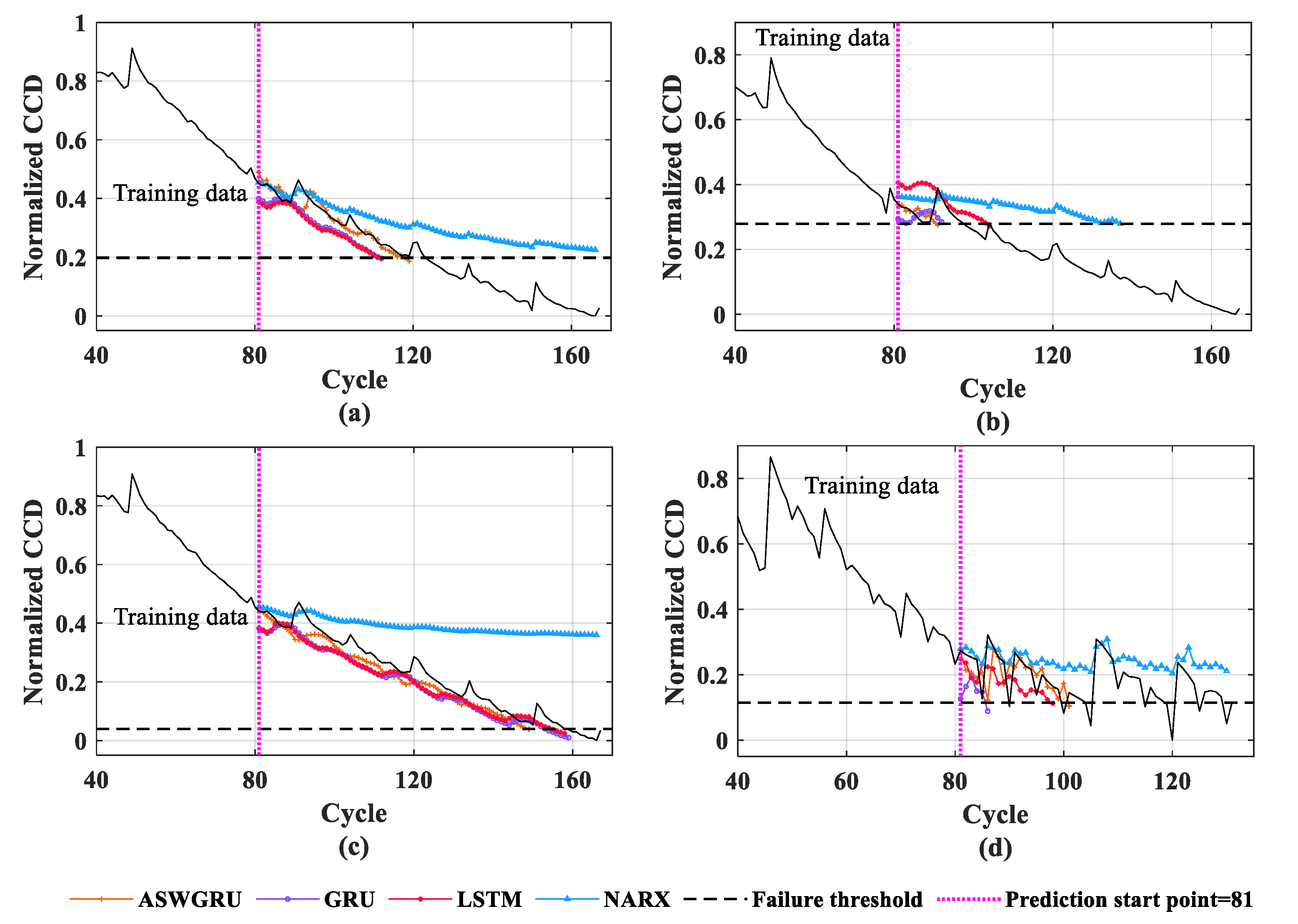
4.2. Performance Assessment
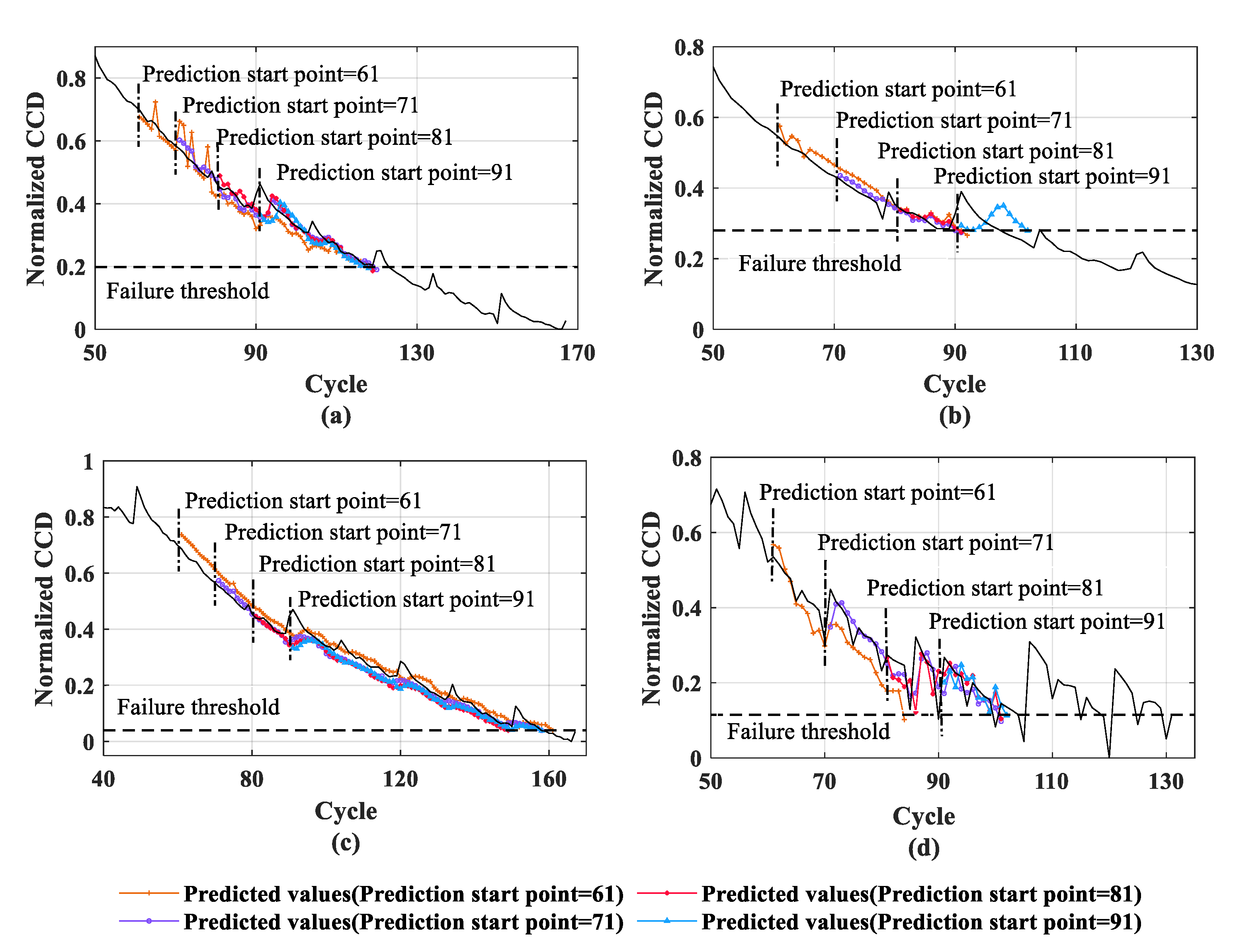
4.3. Prediction Results Analysis
5. Conclusions
Author Contributions
Funding
Institutional Review Board Statement
Informed Consent Statement
Acknowledgments
Conflicts of Interest
References
- Bai, C.; Hu, C.H.; Si, X.H.; Li, H.P.; Zhang, Z.X.; Pei, H. Remaining useful life prediction method for degradation equipment with random shocks. Syst. Eng. Electron. 2018, 40, 2729–2735. [Google Scholar]
- Wang, D.; Miao, Q.; Pecht, M. Prognostics of lithium-ion batteries based on relevance vectors and a conditional three-parameter capacity degradation model. J. Power Sources 2013, 239, 253–264. [Google Scholar] [CrossRef]
- Lu, L.; Han, X.; Li, J.; Hua, J.; Ouyang, M. A review on the key issues for lithium-ion battery management in electric vehicles. J. Power Sources 2013, 226, 272–288. [Google Scholar] [CrossRef]
- Hao, J.; Jing, L.; Ke, H.L.; Wang, Y.; Gao, Q.; Wang, X.X.; Sun, Q.; Xu, Z.J. Determination of cut-off time of accelerated aging test under temperature stress for LED lamps. Front. Inf. Technol. Electron. Eng. 2017, 18, 1197–1205. [Google Scholar] [CrossRef]
- Zhang, Y.; Xiong, R.; He, H.; Pecht, M.G. Lithium-ion battery remaining useful life prediction with Box-Cox transformation and Monte Carlo simulation. IEEE Trans. Ind. Electron. 2019, 66, 1585–1597. [Google Scholar] [CrossRef]
- Cugnet, M.; Sabatier, J.; Laruelle, S.; Grugeon, S.; Sahut, B.; Oustaloup, A.; Tarascon, J.M. On lead-acid-battery resistance and cranking capability estimation. IEEE Trans. Ind. Electron. 2010, 57, 909–917. [Google Scholar] [CrossRef]
- Zou, Y.; Hu, X.; Ma, H.; Li, S.E. Combined state of charge and state of health estimation over lithium-ion battery cell cycle lifespan for electric vehicles. J. Power Sources 2015, 273, 793–803. [Google Scholar] [CrossRef]
- Lipu, M.H.; Hannan, M.A.; Hussain, A.; Hoque, M.M.; Ker, P.J.; Saad, M.M.; Ayob, A. A review of state of health and remaining useful life estimation methods for lithium-ion battery in electric vehicles: Challenges and recommendations. J. Clean. Prod. 2018, 205, 115–133. [Google Scholar] [CrossRef]
- Gomez, J.; Nelson, R.; Kalu, E.E.; Weatherspoon, M.H.; Zheng, J.P. Equivalent circuit model parameters of a high-power Li-ion battery: Thermal and state of charge effects. J. Power Sources 2011, 196, 4826–4831. [Google Scholar] [CrossRef]
- Wei, J.; Dong, G.; Chen, Z. Remaining useful life prediction and state of health diagnosis for lithium-ion batteries using particle filter and support vector regression. IEEE Trans. Ind. Electron. 2018, 65, 5634–5643. [Google Scholar] [CrossRef]
- Sun, Y.; Jou, H.L.; Wu, J. Aging estimation method for lead-acid battery. IEEE Trans. Energy Convers. 2011, 26, 264–271. [Google Scholar] [CrossRef]
- Song, Y.; Liu, D.T.; Hou, Y.D.; Yu, J.; Peng, Y. Satellite lithium-ion battery remaining useful life estimation with an iterative updated RVM fused with the KF algorithm. Chin. J. Aeronaut. 2018, 31, 32–39. [Google Scholar] [CrossRef]
- Liu, D.; Zhou, J.; Liao, H.; Peng, Y.; Peng, X. A health indicator extraction and optimization framework for lithium-ion battery degradation modeling and prognostics. IEEE Trans. Syst. Man Cybern.-Syst. 2015, 45, 915–928. [Google Scholar]
- Widodo, A.; Shim, M.C.; Caesarendra, W.; Yang, B.S. Intelligent prognostics for battery health monitoring based on sample entropy. Expert Syst. Appl. 2011, 38, 11763–11769. [Google Scholar] [CrossRef]
- Chen, L.; Chen, J.; Wang, H.; Wang, Y.; An, J.; Yang, R.; Pan, H. Remaining useful life prediction of battery using a novel indicator and framework with fractional grey model and unscented particle filter. IEEE Trans. Power Electron. 2020, 35, 5850–5859. [Google Scholar] [CrossRef]
- Wu, J.; Zhang, C.; Chen, Z. An online method for lithium-ion battery remaining useful life estimation using importance sampling and neural networks. Appl. Energy 2016, 173, 134–140. [Google Scholar] [CrossRef]
- Patil, M.A.; Tagade, P.; Hariharan, K.S.; Kolake, S.M.; Song, T.; Yeo, T.; Doo, S. A novel multistage Support Vector Machine based approach for Li ion battery remaining useful life estimation. Appl. Energy 2015, 159, 285–297. [Google Scholar] [CrossRef]
- Zhang, Y.; Xiong, R.; He, H.; Pecht, M.G. Long short-term memory recurrent neural network for remaining useful life prediction of lithium-ion batteries. IEEE Trans. Veh. Technol. 2018, 67, 5695–5705. [Google Scholar] [CrossRef]
- Hussein, A.A. Capacity fade estimation in electric vehicle li-ion batteries using artificial neural networks. IEEE Trans. Ind. Appl. 2015, 51, 2321–2330. [Google Scholar] [CrossRef]
- ElSaid, A.; El Jamiy, F.; Higgins, J.; Wild, B.; Desell, T. Optimizing long short-term memory recurrent neural networks using ant colony optimization to predict turbine engine vibration. Appl. Soft Comput. 2018, 73, 969–991. [Google Scholar] [CrossRef] [Green Version]
- Liu, D.; Xie, W.; Liao, H.; Peng, Y. An integrated probabilistic approach to lithium-ion battery remaining useful life estimation. IEEE Trans. Instrum. Meas. 2015, 64, 660–670. [Google Scholar]
- Guo, L.; Li, N.; Jia, F.; Lei, Y.; Lin, J. A recurrent neural network based health indicator for remaining useful life prediction of bearings. Neurocomputing 2017, 240, 98–109. [Google Scholar] [CrossRef]
- Li, X.Y.; Zhang, L.; Wang, Z. Remaining useful life prediction for lithium-ion batteries based on a hybrid model combining the long short-term memory and Elman neural networks. J. Energy Storage 2019, 21, 510–518. [Google Scholar] [CrossRef]
- Cho, K.; van Merriënboer, B.; Gulcehre, C.; Schwenk FB, H.; Bengio, Y. Learning phrase representations using RNN encoder-decoder for statistical machine translation. In Proceedings of the 2014 Conference on Empirical Methods in Natural Language Processing (EMNLP), Doha, Qatar, 25–29 October 2014; pp. 1724–1734. [Google Scholar]
- He, Y.J.; Shen, J.N.; Shen, J.F.; Ma, Z.F. State of health estimation of lithium-ion batteries: A multiscale Gaussian process regression modeling approach. AIChE J. 2015, 61, 1589–1600. [Google Scholar] [CrossRef]
- Zhang, Z.X.; Si, X.S.; Hu, C.H.; Pecht, M.G. A prognostic model for stochastic degrading systems with state recovery: Application to li-ion batteries. IEEE Trans. Reliab. 2017, 66, 1293–1308. [Google Scholar] [CrossRef]
- Saha, B.; Goebel, K. Battery Data Set: NASA Ames Prognostics Data Repository; NASA Ames: Moffett Field, CA, USA, 2007. Available online: https://ti.arc.nasa.gov/tech/dash/groups/pcoe/prognostic-data-repository/ (accessed on 25 August 2021).
- Kadlec, P.; Gabrys, B.; Strandt, S. Data-driven soft sensors in the process industry. Comput. Chem. Eng. 2009, 33, 795–814. [Google Scholar] [CrossRef] [Green Version]
- Yu, J.B. State of health prediction of lithium-ion batteries: Multiscale logic regression and gaussian process regression ensemble. Reliab. Eng. Syst. Saf. 2018, 174, 82–95. [Google Scholar] [CrossRef]
- Gibert, K.; Sevilla-Villanueva, B.; Sànchez-Marrè, M. The role of significance tests in consistent interpretation of nested partitions. J. Comput. Appl. Math. 2016, 292, 623–663. [Google Scholar] [CrossRef]
- Zheng, S.; Kosta, R.; Ahmed, F.; Chetan, G. Long short-term memory network for remaining useful life estimation. In Proceedings of the 2017 IEEE International Conference on Prognostics and Health Management (ICPHM), Dallas, TX, USA, 19–21 June 2017; IEEE: Piscataway, NJ, USA, 2017; pp. 88–95. [Google Scholar]
- Diaconescu, E. The Use of NARX Neural Networks to Predict Chaotic Time Series; World Scientific and Engineering Academy and Society (WSEAS): Dallas, TX, USA, 2008; pp. 182–191. [Google Scholar]
- Pang, X.Q.; Wang, Z.Q.; Zeng, J.C.; Jia, J.F.; Shi, Y.H.; Wen, J. Prediction for the Remaining Useful Life of Lithium-ion Battery Based on PCA-NARX. Trans. Beijing Inst. Technol. 2019, 39, 406–412. [Google Scholar]


| Battery | AT (24 °C) | CC (A) | DC (A) | EOC (V) | EOLC (%) |
|---|---|---|---|---|---|
| B5 | 24 | 1.5 | 2 | 2.7 | 30 |
| B6 | 24 | 1.5 | 2 | 2.5 | 30 |
| B7 | 24 | 1.5 | 2 | 2.2 | 30 |
| B18 | 24 | 1.5 | 2 | 2.5 | 30 |
| Battery | H | Actual Life (Cycles) | |||
|---|---|---|---|---|---|
| B5 | 0.990 **a | 0 | 124 | 1.4 | 0.198 |
| B6 | 0.992 ** | 0 | 101 | 1.4 | 0.279 |
| B7 | 0.989 ** | 0 | 158 | 1.42 | 0.040 |
| B18 | 0.962 ** | 0 | 93 | 1.4 | 0.115 |
| Battery | Methods | Starting Point | R-Square | Real RUL | Predicted RUL | RUL AE |
|---|---|---|---|---|---|---|
| B5 | ASWGRU | 61 | 0.755 | 64 | 59 | 5 |
| 71 | 0.945 | 54 | 51 | 3 | ||
| 81 | 0.944 | 44 | 40 | 4 | ||
| 91 | 0.929 | 34 | 29 | 5 | ||
| GRU | 81 | 0.971 | 44 | 31 | 13 | |
| LSTM | 0.967 | 31 | 13 | |||
| NARX | 0.085 | — | — |
| Battery | Methods | Starting Point | R-Square | Real RUL | Predicted RUL | RUL AE |
|---|---|---|---|---|---|---|
| B6 | ASWGRU | 61 | 0.914 | 41 | 31 | 10 |
| 71 | 0.914 | 31 | 20 | 11 | ||
| 81 | 0.890 | 21 | 10 | 11 | ||
| 91 | 0.852 | 11 | 11 | 0 | ||
| GRU | 81 | 0.923 | 21 | 12 | 9 | |
| LSTM | 0.925 | 24 | 3 | |||
| NARX | −0.797 | 57 | 36 |
| Battery | Methods | Starting Point | R-Square | Real RUL | Predicted RUL | RUL AE |
|---|---|---|---|---|---|---|
| B7 | ASWGRU | 61 | 0.960 | 98 | 100 | 2 |
| 71 | 0.966 | 88 | 91 | 3 | ||
| 81 | 0.944 | 78 | 71 | 7 | ||
| 91 | 0.928 | 68 | 69 | 1 | ||
| GRU | 81 | 0.961 | 78 | 73 | 5 | |
| LSTM | 0.959 | 75 | 3 | |||
| NARX | −1.303 | — | — |
| Battery | Methods | Starting Point | R-Square | Real RUL | Predicted RUL | RUL AE |
|---|---|---|---|---|---|---|
| B18 | ASWGRU | 61 | 0.414 | 33 | 24 | 9 |
| 71 | 0.375 | 23 | 30 | 7 | ||
| 81 | 0.245 | 13 | 20 | 7 | ||
| 91 | 0.203 | 3 | 11 | 8 | ||
| GRU | 81 | 0.019 | 13 | 5 | 8 | |
| LSTM | 0.295 | 18 | 5 | |||
| NARX | −0.575 | — | — |
Publisher’s Note: MDPI stays neutral with regard to jurisdictional claims in published maps and institutional affiliations. |
© 2021 by the authors. Licensee MDPI, Basel, Switzerland. This article is an open access article distributed under the terms and conditions of the Creative Commons Attribution (CC BY) license (https://creativecommons.org/licenses/by/4.0/).
Share and Cite
Wang, Z.; Ma, Q.; Guo, Y. Remaining Useful Life Prediction of Lithium-Ion Batteries Based on Deep Learning and Soft Sensing. Actuators 2021, 10, 234. https://doi.org/10.3390/act10090234
Wang Z, Ma Q, Guo Y. Remaining Useful Life Prediction of Lithium-Ion Batteries Based on Deep Learning and Soft Sensing. Actuators. 2021; 10(9):234. https://doi.org/10.3390/act10090234
Chicago/Turabian StyleWang, Zhuqing, Qiqi Ma, and Yangming Guo. 2021. "Remaining Useful Life Prediction of Lithium-Ion Batteries Based on Deep Learning and Soft Sensing" Actuators 10, no. 9: 234. https://doi.org/10.3390/act10090234
APA StyleWang, Z., Ma, Q., & Guo, Y. (2021). Remaining Useful Life Prediction of Lithium-Ion Batteries Based on Deep Learning and Soft Sensing. Actuators, 10(9), 234. https://doi.org/10.3390/act10090234