3.1. L2 State Gain Feedback Control
The non-homogeneous state equation of the closed-loop linear system is defined as
Let the feedback control input be
, and substitute it into Equations (42) and (43),
According to the principle of
state gain feedback control [
30,
31,
32], the
gain of the closed-loop system should be less than any positive number
,
Therefore,
is the upper bound of the
gain of the closed-loop system. When the above condition is satisfied, in order to ensure the stability of the feedback system, it needs to be met,
where
is the second-order Lyapunov function, and its expression is
where
is a symmetric positive definite matrix. Substituting Equations (44), (45), and (48) into the linear matrix inequality (47),
Let
, then Equation (49) can be expressed as
where
.
Suppose the partition matrix
, where
is non-zero value, then the Schur complement matrix of the partition matrix
with respect to
is
Since the matrix
satisfies the form of Equation (51), namely,
Then, the matrix
is rewritten as a Schur complement matrix and substituted into Equation (50),
where
indicates that the partition matrix
is a negative definite matrix.
Multiply both sides of the matrix
by the diagonal matrix
respectively, and let
and
to get
Therefore, according to the analysis in this section, is the upper bound of the state feedback gain of the system at all times. The magnitude of feedback control force is closely related to . In order to make the system have a good control effect, the problem of solving the state gain can be transformed into a linear matrix inequality problem of solving the minimum value of .
3.2. L2 State Gain of the Driver-Active Suspension Model
In order to improve the ride comfort, according to the international standard file ISO 2631, take the acceleration of the head and neck, the acceleration of the hip and thigh (that is, the seat support surface), the pitch angle acceleration, the body acceleration of the front axle, the suspension working space of the front axle, the dynamic tire deflection of the front tire, the body acceleration of the rear axle, the suspension working space of the rear axle and the dynamic tire deflection of the rear tire as performance indexes, that is,
where
is the weighting coefficient matrix of each performance index, and its value is the tendency of control rule to each performance index.
According to the performance index variables, the state index equation of the system is established as follows:
where
is the output state coefficient matrix,
is the input–output coupling matrix,
According to the above
state gain feedback control algorithm, taking the Ford Granada as an example, the driver’s active suspension model is established. The parameters of the established active suspension system model are shown in
Table 1, and the parameters of the established driver model are shown in
Table 2.
The performance index of vehicle suspension system will change with the change of weighting coefficient. Therefore, the determination of the weighting coefficient determines the control effect of the controller. In this paper, genetic algorithm is used to solve the weighting coefficient by referring to references [
33,
34]. The algorithm flow is shown in
Figure 3.
The order of magnitude and the unit of the nine performance indexes of the driver seat-active suspension is different. For normalization comparison, the fitness function of genetic algorithm is set to
The constraint condition is
where
is the root mean square value of the 9 performance indicators of the system,
is the performance index of active suspension,
is the performance index of passive suspension,
is the weighting coefficient matrix of each performance index.
Set the initial search range of the genetic algorithm. The range of is [1, 1], the range of is [1, 1000], the range of is [1, 1000], the range of is [1, 1000], the range of is [1000, 10,000], the range of is [1000, 10,000], the range of is [1, 1000], the range of is [10,000, 50,000] and the range of is [10,000, 50,000].
The weighting coefficients of the performance index of the
state gain feedback control in this paper are obtained in
Figure 4.
The weighting coefficients
According to the model parameters established in this paper, through solving the linear matrix inequality of the driver-active suspension model, the minimum value of the upper bound
of
gain of the closed-loop system satisfying the inequality (54) is 13.686. The corresponding
state gain feedback matrix is
where
3.3. Energy Consumption of Multi-Link Active Suspension
The structure diagram of the multi-link active suspension is shown in
Figure 5.
As shown in
Figure 5a,b, the relationship between the axial control force of the real suspension actuator and the vertical control force in the simplified model is
Then, the real active control force of the actuator is
The relationship between the height of the suspension and the rotation angle of the lower platform is
where
is the suspension height,
is the length of the link, that is, the original height of the suspension,
is the distance from the center of the link to the center of the platform and
is the angle of rotation of the platform relative to the original position.
For a single active suspension, according to the law of conservation of energy, it can be known that
where
is the vertical equivalent active control force,
is the suspension height without active control force,
is the suspension height with active control force,
is the torque of the lower platform,
is the angle of rotation of the lower platform without active control force,
is the angle of rotation of the lower platform with active control force,
is the weight of the body and the upper platform of the suspension,
is the number of link, and
is the weight of a single link.
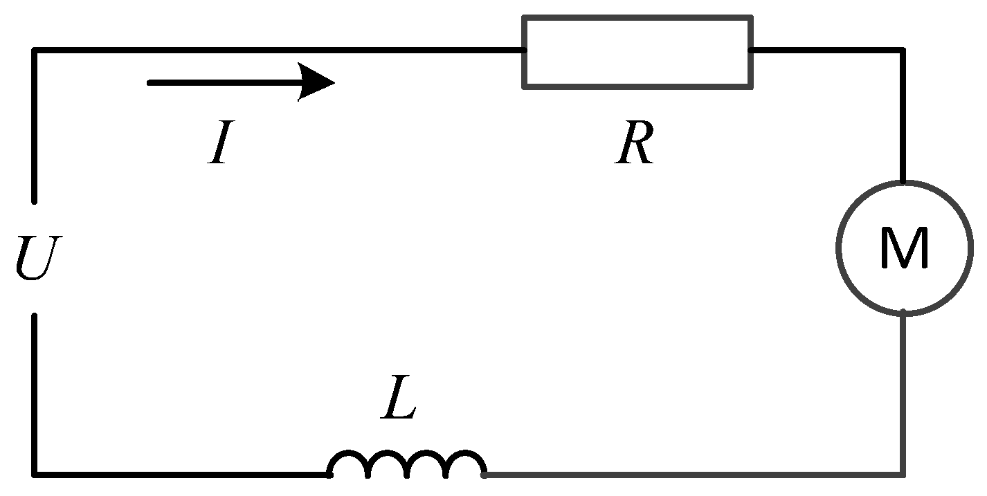
The circuit diagram of the active suspension actuator is shown in
Figure 6, where
is the permanent magnet brushless DC,
is the inductor,
is the supply voltage,
is the armature circuit current, and
is the armature circuit internal resistance.
The relationship between the torque required by the suspension lower platform and the motor output torque is
where
is the torque transfer coefficient,
is the motor output torque,
is the transmission efficiency of the mechanism, and
is the transmission ratio of the growth mechanism.
The parameter nature of the actuator is
where
is the electromotive force of the motor,
is the axial speed of suspension,
is the suspension conversion to drive motor constant,
is active control force.
where
is the motor torque constant.
The motor equations are
where
is the rated power of the motor,
is the number of electric drive conductors,
is the pole log of the motor,
is the logarithm of the parallel branches,
is the magnetic flux passing through the coil,
is rated motor speed,
is the outer diameter,
is air gap magnetic density,
is the electric drive length, and
is rated power of the motor.
The relationship between active control force
and current
is
where
is the ratio of electric drive length to outside diameter and
is the radius of the rotating platform.
where
is the outer diameter correction factor,
is the apparent power,
is the polar arc coefficient,
is electrical load, and
is the short moment coefficient.
The real parameters of the multi-link active suspension motor are shown in
Table 3.
According to the motor and structural parameters, is calculated.
According to the energy consumption calculation method [
35,
36], for the model established in this paper, the total energy consumption power of the multi-link active suspension
is
where
is the power consumed by the front axle active suspension,
is the power consumed by the rear axle active suspension,
is the active control force of the front axle suspension, and
is the active control force of the rear axle suspension.
Then the energy consumption power used by the active element to control vibration per each unit of mass is
3.4. Simulation and Experiment of Active Suspension
According to the above
state gain feedback control algorithm and model parameters, a 9-DOF driver seat-active suspension model, a driver seat-passive suspension model and a traditional LQG semi-vehicle active suspension model that do not consider the driver are established, respectively. The suspension model is simulated by using the class B road conditions and
vehicle speed conditions in the international standardization document ISO/TC 108/SC2N67. The active control force and energy consumption power of front axle and rear axle actuators based on
L2 control driver model and traditional LQG algorithm [
18] are shown in
Figure 7.
According to
Figure 7a curve, the RMS values of the active control force of the front axle and rear axle actuators of the driver seat-active suspension are 265.79 N and 390.68 N, respectively. The RMS values of the active control force of the LQG active suspension are 255.02 N and 429.81 N, respectively.
It can be seen from
Figure 7b, the mean value of the energy consumption power of the front axle actuator of the driver seat-active suspension is 77.6034 W, the mean value of the LQG front axle actuator is 55.1376 W, the mean value of the energy consumption power of the rear axle actuator of the driver seat-active suspension is 47.2937 W and the mean value of the LQG rear axle actuator is 132.3449 W. The new control algorithm can decrease the total energy cost from 180 W to 133 W. According to Equation (70), the mean value of power consumed per unit of sprung mass is 0.1523 W/Kg less than 0.2286 W/Kg of LQG algorithm. Compared with the LQG control algorithm, the algorithm established in this paper has a better energy consumption.
According to Equations (63) and (69), the drive current response curve of the active suspension drive motor is obtained, and as shown in
Figure 8.
It can be seen from
Figure 8, the driving current required by the front and rear axle actuators is less than 15 A, within the rated current range. A positive current means that the direction of the active control force is upward, and vice versa. By calculation, the RMS value of the driving current of the front axle actuator is 2.5951 A. The RMS value of the driving current of the rear axle actuator is 4.3737 A.
The simulation results of the semi-vehicle 9-DOF driver seat-active suspension model, the LQG semi-vehicle-active suspension model without considering the driver and the driver seat-passive suspension model are shown in
Figure 9. The RMS values and the absolute value of the mean value of the performance indexes of the three different models are calculated respectively, and as shown in
Table 4. After the energy supplement system has been designed, the control efficiency could be calculated using the ratio between the currents or powers.
It can be seen from
Figure 9 and
Table 4 that the system model and control algorithm established in this paper can significantly improve the ride comfort of the driver. Compared with the passive suspension and the LQG active suspension without considering the driver, the RMS value of the acceleration on the driver’s head is respectively reduced by 27.5% and 10.9%. The RMS value of the acceleration on the driver’s hip and thigh (that is, the seat support surface) is, respectively, reduced by 29.9% and 15.9%. The RMS value of the pitch angle acceleration experienced by the driver is reduced by 27.2% and 6.4%, respectively. The RMS value of the acceleration on the driver’s waist is respectively reduced by 28.7% and 6.7%. The RMS value of the acceleration on the driver’s chest is respectively reduced by 27.7% and 7.5%. Compared with the passive suspension, the absolute value of the mean value of these five performance indexes decreased by 94.5%, 89.5%, 26.9%, 89.2%, and 90.1%, respectively. Compared with the LQG active suspension without considering the driver, the absolute value of the mean value of these five performance indexes respectively decreased by 50.0%, 20.0%, 38.7%, 58.8%, and 61.9%.
In addition, the
state gain feedback control has an ideal control effect on suspension and passive components of the body. After the driver–seat–suspension model adopts the
state gain feedback active control, compared with the passive suspension and the LQG active suspension without considering the driver, the RMS value of the body acceleration of the front axle is respectively reduced by 19.3% and 1.3%. The RMS value of the body acceleration of the rear axle is respectively reduced by 22.0% and 5.8%. The RMS value of the dynamic tire deflection of the front tire is respectively reduced by 6.5% and 32.6%. The RMS value of the dynamic tire deflection of the rear tire is respectively reduced by 3.3% and 12.1%. There is a coupling relationship between the body acceleration and the suspension working space. When the body acceleration is greatly increased, the suspension working space will deteriorate. According to the weighted factor optimization of
control algorithm in
Section 3.2, although the suspension working space of front axle and rear axle is not significantly optimized, compared with the LQG active suspension without considering the driver, the suspension working space of front axle and rear axle is respectively reduced by 22.2% and 35.9%.
In order to further verify the influence of the model and control algorithm established in this paper on driving comfort, the power spectral density function is obtained by spectrum analysis of acceleration of the driver’s head and neck, acceleration of the driver’s hip and thigh, and pitch angle acceleration. The power spectrum estimation of the performance index in the time domain is estimated by periodogram method.
where
is the power spectral density of random sequence at the corresponding frequency
,
is random sequence,
is the number of random sequence data in the time domain, and
is the sampling signal frequency. In this paper, the sampling time interval is
, so
. The power spectral density functions of the three performance indicators are shown in
Figure 10.
It can be seen from
Figure 10, the passive suspension and driver seat-active suspension have roughly the same waveforms. The power spectral density of acceleration on the driver’s head and neck and acceleration on the driver’s hip and thigh are all concentrated in the frequency range of 0 to 10 Hz, and there are two peaks within this frequency range. The power spectral density of the pitch angular acceleration mainly concentrates in the frequency range of 0 to 20 Hz, and the peak value appears in the frequency range of 0 to 10 Hz and 10–20 Hz, respectively.
The power spectrum density function obtained above is frequency-weighted according to the international standard document ISO 2631, and the RMS value of the weighted acceleration of the driver seat-active suspension is and the RMS value of the weighted acceleration of the passive suspension is , so that the driver is in a relatively comfortable range in the driver seat-active suspension system, and in a relatively uncomfortable range in the passive suspension system. Therefore, the driving comfort of the driver can be improved after the the state gain feedback control is adopted in vehicle suspension.


