
A Deep Reinforcement Learning Algorithm Based on Tetanic Stimulation and Amnesic Mechanisms for Continuous Control of Multi-DOF Manipulator


Abstract
:1. Introduction
2. Related Work
3. Methods
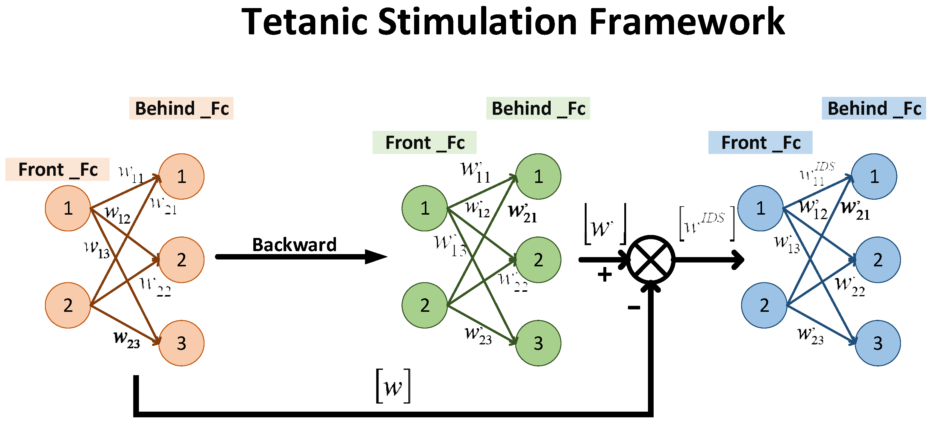
3.1. Tetanic Stimulation
| Algorithm 1 Tetanic stimulation |
| 1: Tetanic stimulation coefficient 2: Load Actor network , 3: Update Actor network 4: Load New Actor network, 5: 6: Select the serial number of the T largest data in 7: For t = 1 to T do: 8: If : 9: If 10: 11: else: 12: 13: End if 14: End if 15: End for |
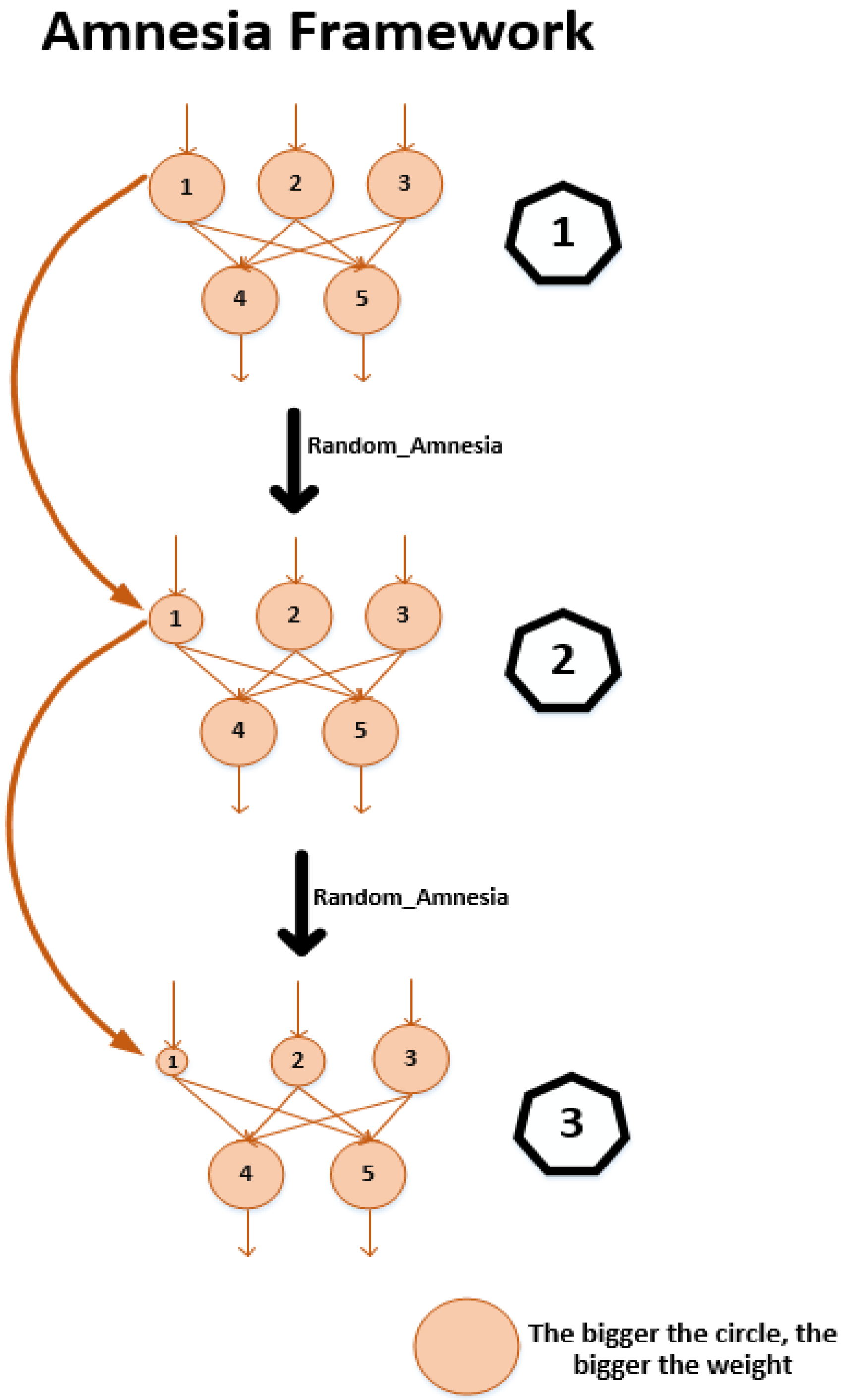
3.2. Amnesia Mechanism
| Algorithm 2 Amnesia Framework |
| 1: Load Actor network, 2: is the number of the ’s node 3: For i = 1 to : 4: Random(0, 1) number , Amnesia threshold value , Mutation coefficient 5: If : 6: 7: End if 8: End for |
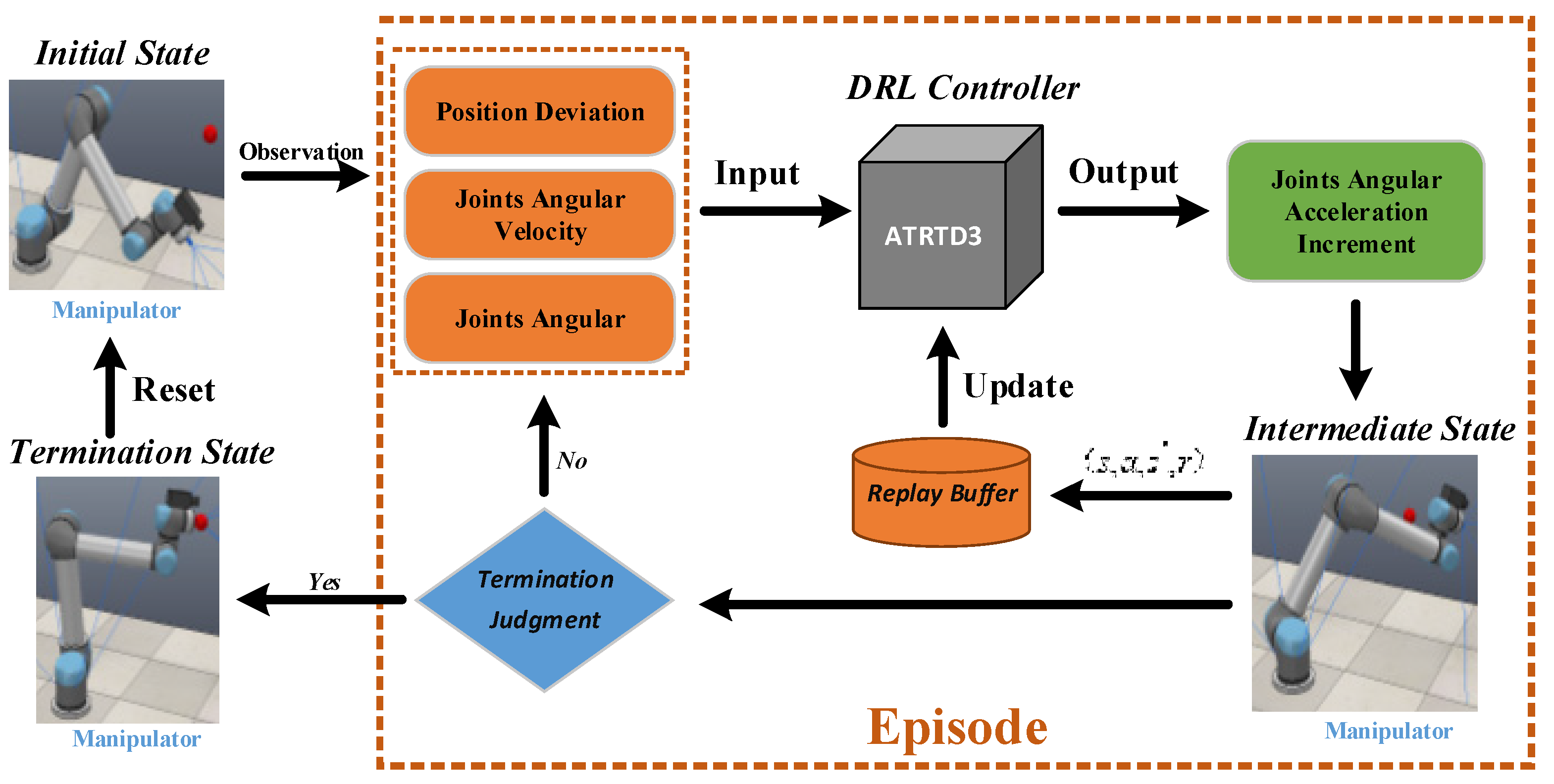
4. Experiment
4.1. Experiment Setup
4.2. Task Introduction
4.3. Simulation Environment Construction
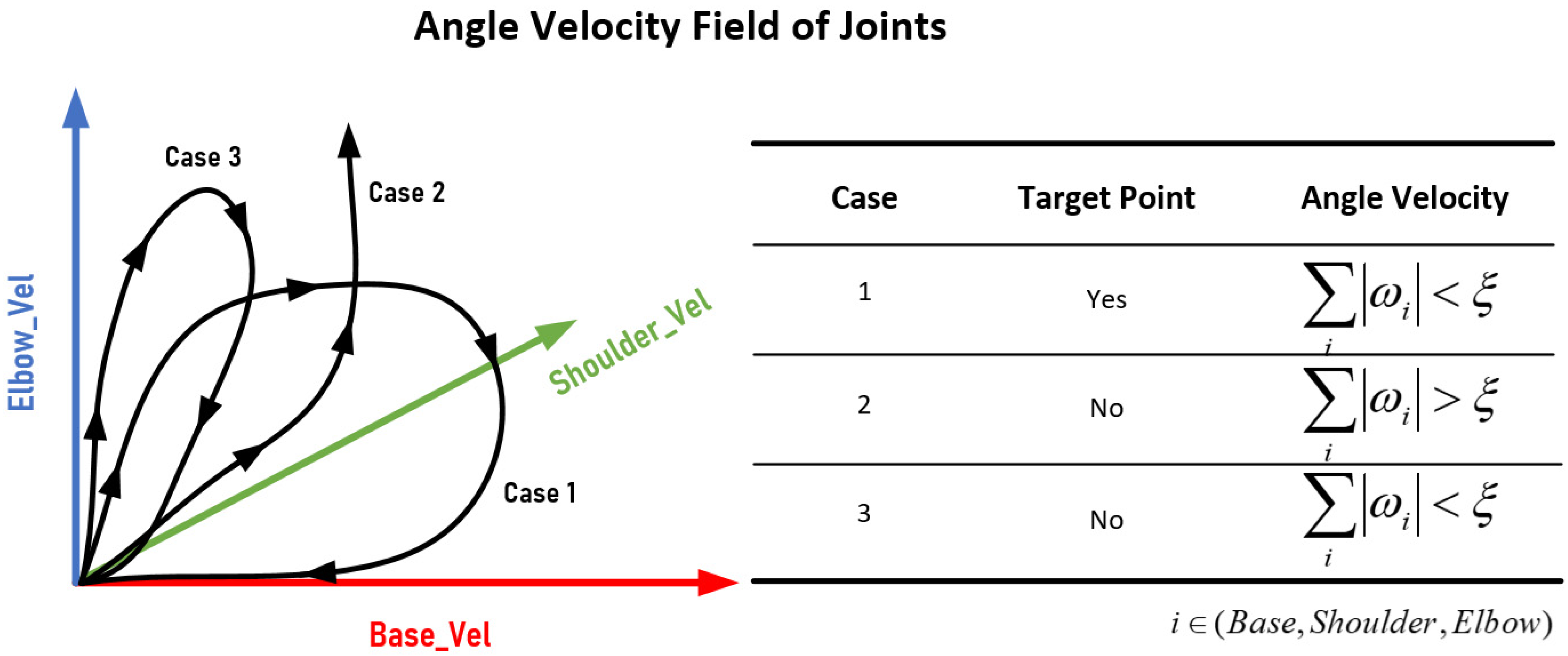
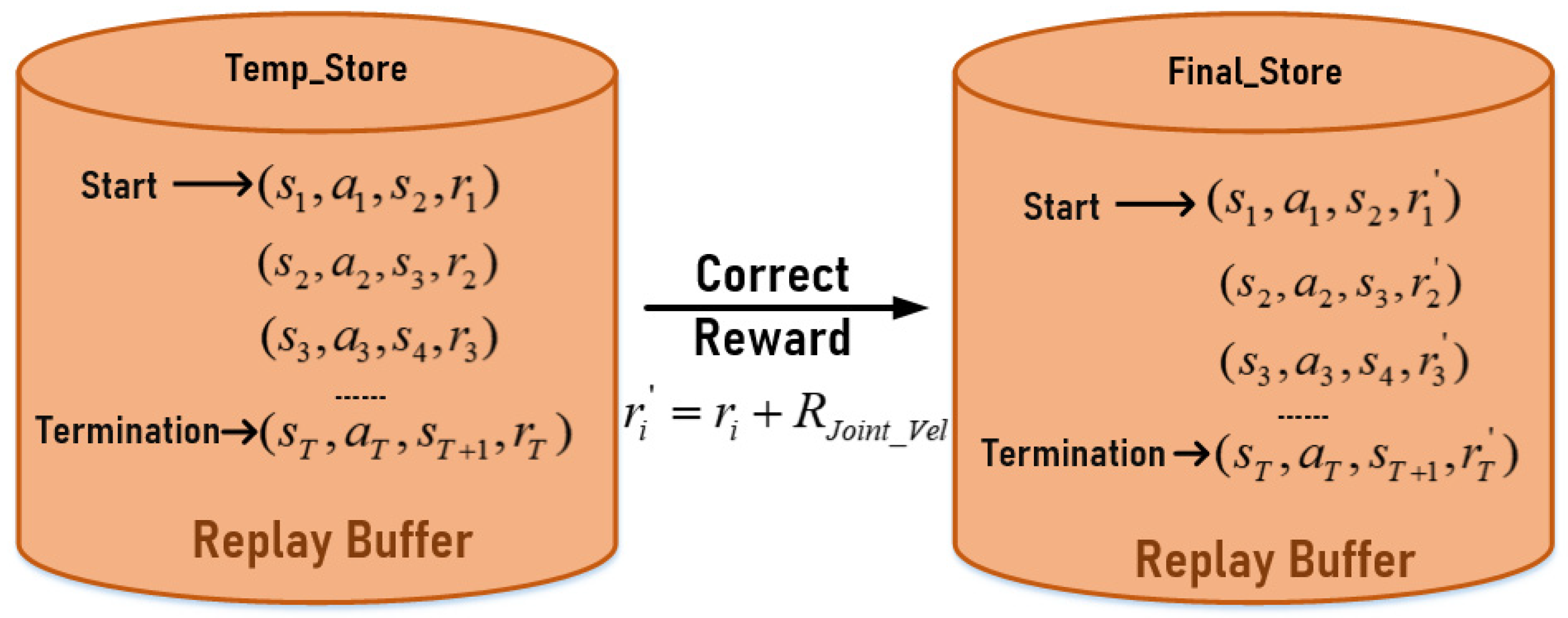
4.4. Rewriting Experience Playback Mechanism and Reward Function Design
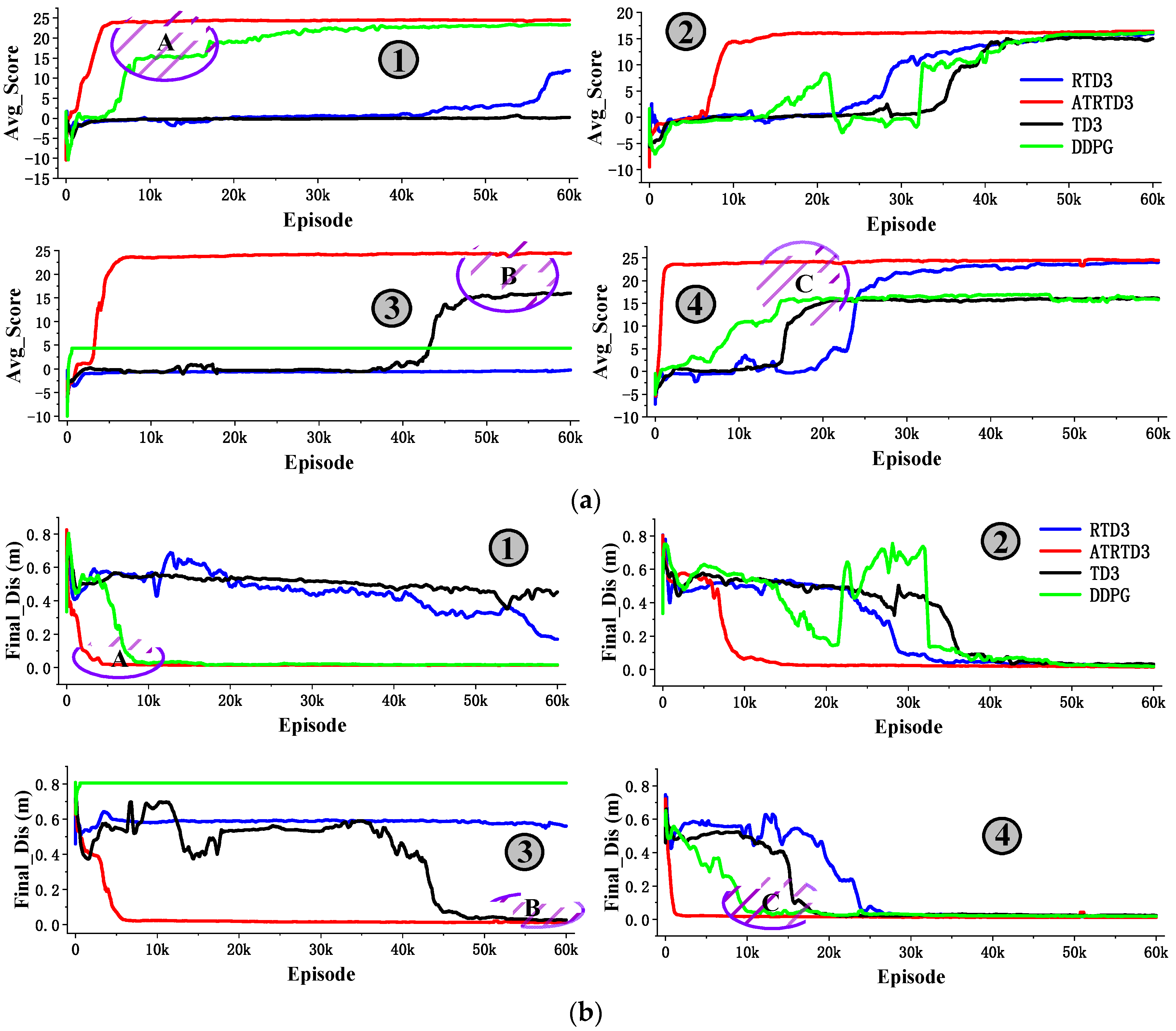
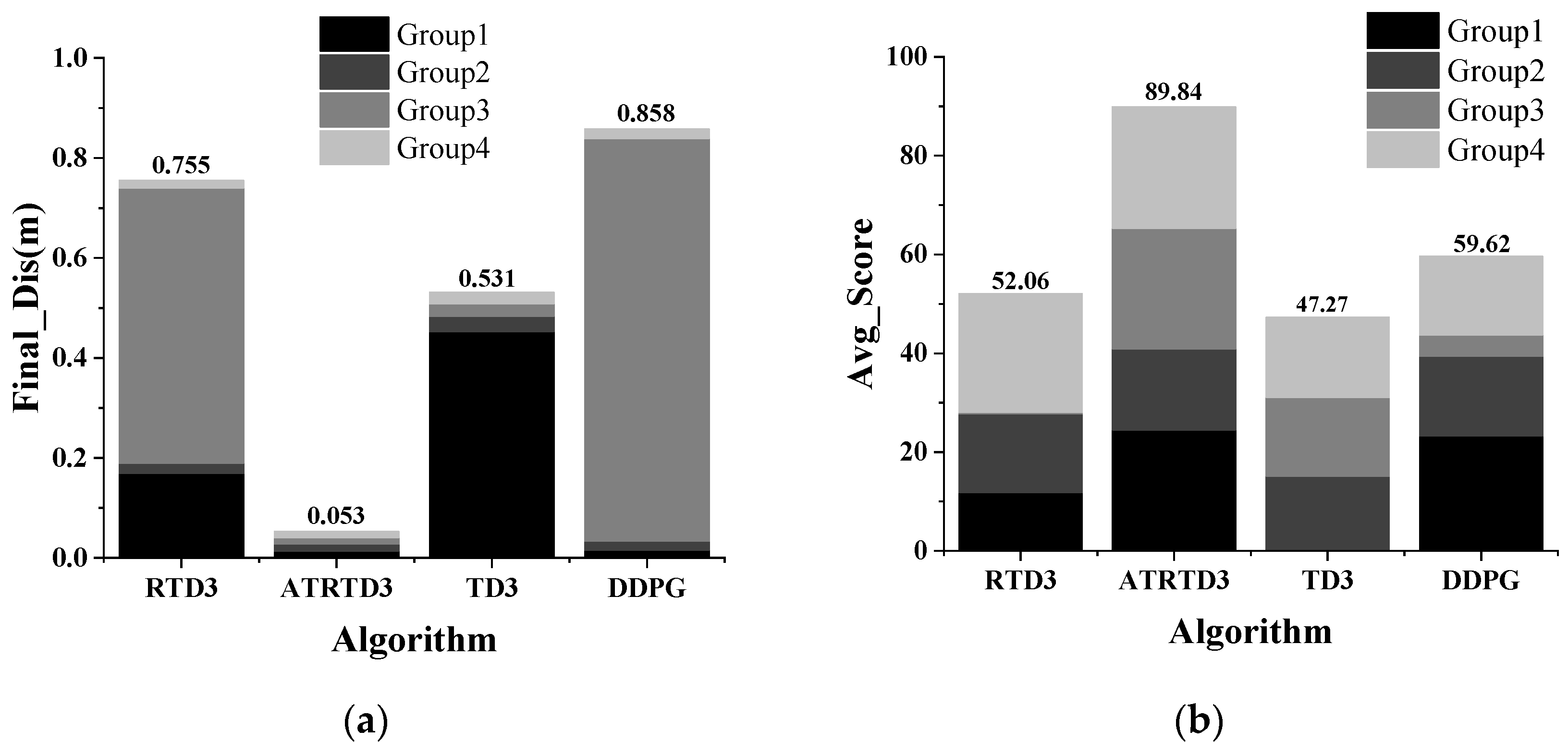
4.5. Simulation Experimental Components
5. Discussion
6. Conclusions
Author Contributions
Funding
Institutional Review Board Statement
Informed Consent Statement
Data Availability Statement
Conflicts of Interest
Appendix A
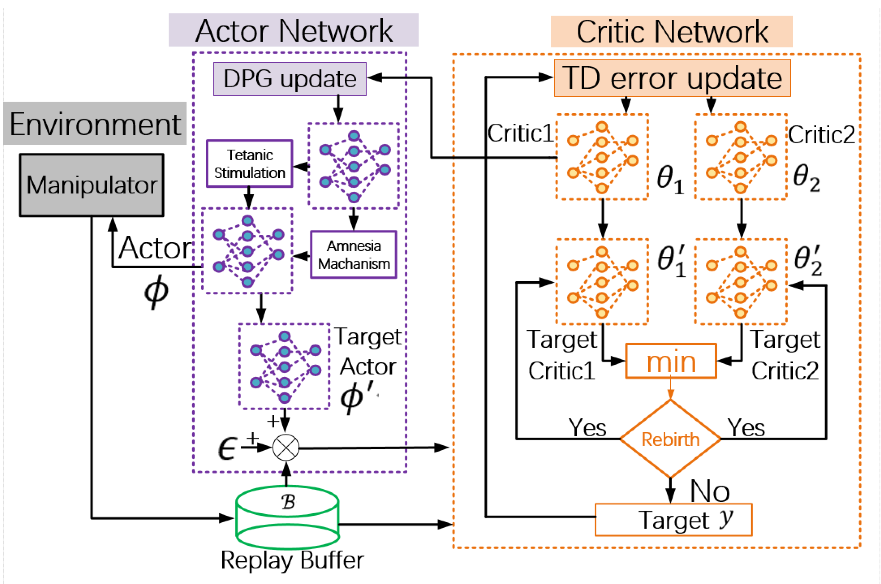
| Algorithm A1. ATRTD3 |
| 1: Initialize critic networks ,and actor network with random parameters 2: Initialize target networks 3: Target network node assignment 4: Initialize replay buffer 5: for to do 6: Amnesia framework 7: Select action with exploration noise 8: Temporary store transition tuple in 9: Fix transition tuple , angular velocity correction 10: Store transition tuple in 11: If then 12 return 13: Sample mini-batch of transition from 14: 15: 16: Statistical calculation of value utilization ratio , 17: If then 18: Rebirth target networks 19: End if 20: If then 21: Rebirth target networks 22: End if 23: Update critics 24: If mod then 25: Update by the deterministic policy gradient: 26: 27: Tetanic stimulation Framework 28: Update target networks: 29: 30: 31: End if 32: End if 33: End for |
References
- Levine, S.; Pastor, P.; Krizhevsky, A.; Ibarz, J.; Quillen, D. Learning Hand-Eye Coordination for Robotic Grasping with Large-Scale Data Collection. In International Symposium on Experimental Robotics; Springer: Cham, Switzerland, 2016; pp. 173–184. [Google Scholar]
- Zhang, M.; Mccarthy, Z.; Finn, C.; Levine, S.; Abbeel, P. Learning deep neural network policies with continuous memory states. In Proceedings of the International Conference on Robotics and Auto-mation, Stockholm, Sweden, 16 May 2016; pp. 520–527. [Google Scholar]
- Levine, S.; Finn, C.; Darrell, T.; Abbeel, P. End-to-end training of deep visuomotor policies. J. Mach. Learn. Res. 2016, 17, 1–40. [Google Scholar]
- Lenz, I.; Knepper, R.; Saxena, A. DeepMPC:learning deep latent features for model predictive control. In Proceedings of the Robotics Scienceand Systems, Rome, Italy, 13–17 July 2015; pp. 201–209. [Google Scholar]
- Satija, H.; Pineau, J. Simultaneous machine translation using deep reinforcement learning. In Proceedings of the Workshops of International Conference on Machine Learning, New York, NY, USA, 24 June 2016; pp. 110–119. [Google Scholar]
- Sallab, A.; Abdou, M.; Perot, E.; Yogamani, S. Deep reinforcement learning framework for autonomous driving. Electron. Imaging 2017, 19, 70–76. [Google Scholar] [CrossRef] [Green Version]
- Caicedo, J.; Lazebnik, S. Active Object Localization with Deep Reinforcement Learning. In Proceedings of the IEEE International Conference on Computer Vision, Santiago, Chile, 11–18 December 2015; pp. 2488–2496. [Google Scholar]
- Mnih, V.; Kavukcuoglu, K.; Silver, D.; Graves, A.; Antonoglou, I.; Wierstra, D.; Riedmiller, M. Playing Atari with Deep Reinforcement Learning. arXiv 2013, arXiv:1312.5602. [Google Scholar]
- Mnih, V.; Kavukcuoglu, K.; Silver, D.; Rusu, A.A.; Veness, J.; Bellemare, M.G.; Graves, A.; Riedmiller, M.; Figjeland, A.K.; Ostrovski, G.; et al. Human-level control through deep reinforcement learning. Nature 2015, 518, 529–533. [Google Scholar] [CrossRef]
- Lillicrap, T.; Hunt, J.; Pritzel, A.; Heess, N.; Erez, T.; Tassa, Y.; Silver, D.; Wierstra, D. Continuous control with deep reinforcement learning. arXiv 2015, arXiv:1509.02971. [Google Scholar]
- Schulman, J.; Levine, S.; Moritz, P.; Jordan, M.I.; Abbeel, P. Trust Region Policy Optimization. In Proceedings of the International Conference on Machine Learning, Lille, France, 6–11 July 2015; pp. 1889–1897. [Google Scholar]
- Mnih, V.; Badia, A.; Mirza, M.; Graves, A.; Lillicrap, T.; Harley, T.; Silver, D.; Kavukcuoglu, K. Asynchronous methods for deep reinforcement learning. In Proceedings of the International Conference on Machine Learning, New York, NY, USA, 19–24 June 2016; pp. 1928–1937. [Google Scholar]
- Schulman, J.; Wolski, F.; Dhariwal, P.; Radford, A.; Klimov, O. Proximal Policy Optimization Algorithms. arXiv 2017, arXiv:1707.06347. [Google Scholar]
- Heess, N.; Dhruva, T.B.; Sriram, S.; Lemmon, J.; Silver, D. Emergence of Locomotion Behaviours in Rich Environments. arXiv 2017, arXiv:1707.02286. [Google Scholar]
- Fujimoto, S.; Hoof, H.V.; Meger, D. Addressing function approximation error in actor-critic methods. In Proceedings of the 35th International Conference on Machine Learning, Stockholm, Sweden, 10–15 July 2018; pp. 1587–1596. [Google Scholar]
- Fortunato, M.; Azar, M.G.; Piot, B.; Menick, J.; Osband, I.; Graves, A.; Mnih, V.; Munos, R.; Hassabis, D.; Pietquin, O.; et al. Noisy Networks for Exploration. arXiv 2017, arXiv:1706.10295. [Google Scholar]
- Plappert, M.; Houthooft, R.; Dhariwal, P.; Sidor, S.; Chen, R.Y.; Chen, X.; Asfour, T.; Abbeel, P.; Andrychowicz, M. Parameter Space Noise for Exploration. arXiv 2017, arXiv:1706.01905. [Google Scholar]
- Bellemare, M.; Srinivasan, S.; Ostrovski, G.; Schaul, T.; Saxton, D.; Munos, R. Unifying count-based exploration and intrinsic motivation. Adv. Neural Inf. Process. Syst. 2016, 29, 1471–1479. [Google Scholar]
- Choshen, L.; Fox, L.; Loewenstein, Y. DORA The Explorer: Directed Outreaching Reinforcement Action-Selection. arXiv 2018, arXiv:1804.04012. [Google Scholar]
- Badia, A.; Sprechmann, P.; Vitvitskyi, A.; Guo, D.; Piot, B.; Kapturowski, S.; Tieleman, O.; Arjovsky, M.; Pritzel, A.; Bolt, A.; et al. Never Give Up: Learning Directed Exploration Strategies. arXiv 2020, arXiv:2002.06038. [Google Scholar]
- Gu, S.; Holly, E.; Lillicrap, T.; Levine, S. Deep Reinforcement Learning for Robotic Manipulation with Asynchronous Off-Policy Updates. arXiv 2016, arXiv:1610.00633. [Google Scholar]
- Hassabis, D.; Kumaran, D.; Summerfield, C.; Botvinick, M. Neuroscience-Inspired Artificial Intelligence. Neuron 2017, 95, 245–258. [Google Scholar] [CrossRef] [Green Version]
- MyeongSeop, K.; DongKi, H.; JaeHan, P.; JuneSu, K. Motion Planning of Robot Manipulators for a Smoother Path Using a Twin Delayed Deep Deterministic Policy Gradient with Hindsight Experience Replay. Appl. Sci. 2020, 10, 575. [Google Scholar]
- Zhang, H.; Wang, F.; Wang, J.; Cui, B. Robot Grasping Method Optimization Using Improved Deep Deterministic Policy Gradient Algorithm of Deep Reinforcement Learning. Rev. Sci. Instrum. 2021, 92, 1–11. [Google Scholar]
- Kwiatkowski, R.; Lipson, H. Task-agnostic self-modeling machines. Sci. Robot. 2019, 4, eaau9354. [Google Scholar] [CrossRef]
- Iriondo, A.; Lazkano, E.; Susperregi, L.; Urain, J.; Fernandez, A.; Molina, J. Pick and Place Operations in Logistics Using a Mobile Manipulator Controlled with Deep Reinforcement Learning. Appl. Sci. 2019, 9, 348. [Google Scholar] [CrossRef] [Green Version]
- Giorgio, I.; Del Vescovo, D. Energy-based trajectory tracking and vibration control for multilink highly flexible manipulators. Math. Mech. Complex Syst. 2019, 7, 159–174. [Google Scholar] [CrossRef] [Green Version]
- Rubinstein, D. Dynamics of a flexible beam and a system of rigid rods, with fully inverse (one-sided) boundary conditions. Comput. Methods Appl. Mech. Eng. 1999, 175, 87–97. [Google Scholar] [CrossRef]
- Bliss, T.V.P.; Lømo, T. Long-lasting potentiation of synaptic transmission in the dentate area of the anaesthetized rabbit following stimulation of the perforant path. J. Physiol. 1973, 232, 331–356. [Google Scholar] [CrossRef]
- Hebb, D.O. The Organization of Behavior; Wiley: New York, NY, USA, 1949. [Google Scholar]
- Thomas, M.J.; Watabe, A.M.; Moody, T.D.; Makhinson, M.; O’Dell, T.J. Postsynaptic Complex Spike Bursting Enables the Induction of LTP by Theta Frequency Synaptic Stimulation. J. Neurosci. 1998, 18, 7118–7126. [Google Scholar] [CrossRef] [PubMed]
- Dayan, P.; Abbott, L.F. Theoretical Neuroscience: Computational and Mathematical Modeling of Neural Systems; The MIT Press: New York, NY, USA, 2001. [Google Scholar]
- Bliss, T.V.P.; Cooke, S.F. Long-Term Potentiation and Long-Term Depression: A Clinical Perspective. Clinics 2011, 66 (Suppl. 1), 3–17. [Google Scholar] [CrossRef] [Green Version]
- Hou, Y.Y.; Hong, H.J.; Sun, Z.M.; Xu, D.S.; Zeng, Z. The Control Method of Twin Delayed Deep Deterministic Policy Gradient with Rebirth Mechanism to Multi-DOF Manipulator. Electronics 2021, 10, 870. [Google Scholar] [CrossRef]
- Denavit, J.; Hartenberg, R.S. A Kinematic Notation for Lower-Pair Mechanisms. J. Appl. Mech. 1955, 77, 215–221. [Google Scholar] [CrossRef]


| Joint | ||||
|---|---|---|---|---|
| Base | 0 | 0.0892 | ||
| Shoulder | −0.4250 | 0 | 0 | |
| Elbow | −0.3923 | 0 | 0 | |
| Wrist1 | 0 | 0.1092 | ||
| Wrist2 | 0 | 0.0946 | ||
| Wrist3 | 0 | 0.0823 | 0 |
| Joint | Base | Shoulder | Elbow | |||
|---|---|---|---|---|---|---|
| Angular Velocity | Average (rad/s) | Var | Average (rad/s) | Var | Average (rad/s) | Var |
| ATRTD3 | −2.50 × 10⁻³ | 2.80 × 10⁻⁵ | 2.51 × 10⁻³ | 3.09 × 10⁻⁵ | −3.90 × 10⁻⁴ | 2.83 × 10⁻⁵ |
| RTD3 | −4.65 × 10⁻³ | 4.58 × 10⁻⁴ | −3.13 × 10⁻² | 1.07 × 10⁻³ | 3.35 × 10⁻³ | 6.81 × 10⁻⁴ |
| TD3 | 3.13 × 10⁻² | 7.26 × 10⁻⁴ | −2.79 × 10⁻² | 1.32 × 10⁻³ | −6.69 × 10⁻³ | 4.73 × 10⁻⁴ |
| DDPG | 2.66 × 10⁻³ | 4.60 × 10⁻⁵ | 2.52 × 10⁻² | 6.41 × 10⁻⁵ | −2.01 × 10⁻² | 3.95 × 10⁻⁵ |
| Joint | Base | Shoulder | Elbow | |||
|---|---|---|---|---|---|---|
| Angular Velocity | Average (rad/s) | Var | Average (rad/s) | Var | Average (rad/s) | Var |
| ATRTD3 | −1.71 × 10⁻² | 4.17 × 10⁻⁵ | 8.04 × 10⁻³ | 1.08 × 10⁻⁴ | −1.23 × 10⁻² | 6.18 × 10⁻⁵ |
| RTD3 | 3.03 × 10⁻² | 1.14 × 10⁻⁴ | −2.50 × 10⁻³ | 5.87 × 10⁻⁴ | −1.73 × 10⁻² | 4.48 × 10⁻⁴ |
| TD3 | 1.39 × 10⁻² | 3.40 × 10⁻⁵ | 3.67 × 10⁻² | 9.69 × 10⁻⁵ | −6.58 × 10⁻² | 6.95 × 10⁻⁵ |
| DDPG | 3.20 × 10⁻² | 5.38 × 10⁻⁵ | −1.40 × 10⁻² | 7.07 × 10⁻⁵ | 8.21 × 10⁻³ | 1.27 × 10⁻⁴ |
Publisher’s Note: MDPI stays neutral with regard to jurisdictional claims in published maps and institutional affiliations. |
© 2021 by the authors. Licensee MDPI, Basel, Switzerland. This article is an open access article distributed under the terms and conditions of the Creative Commons Attribution (CC BY) license (https://creativecommons.org/licenses/by/4.0/).
Share and Cite
Hou, Y.; Hong, H.; Xu, D.; Zeng, Z.; Chen, Y.; Liu, Z. A Deep Reinforcement Learning Algorithm Based on Tetanic Stimulation and Amnesic Mechanisms for Continuous Control of Multi-DOF Manipulator. Actuators 2021, 10, 254. https://doi.org/10.3390/act10100254
Hou Y, Hong H, Xu D, Zeng Z, Chen Y, Liu Z. A Deep Reinforcement Learning Algorithm Based on Tetanic Stimulation and Amnesic Mechanisms for Continuous Control of Multi-DOF Manipulator. Actuators. 2021; 10(10):254. https://doi.org/10.3390/act10100254
Chicago/Turabian StyleHou, Yangyang, Huajie Hong, Dasheng Xu, Zhe Zeng, Yaping Chen, and Zhaoyang Liu. 2021. "A Deep Reinforcement Learning Algorithm Based on Tetanic Stimulation and Amnesic Mechanisms for Continuous Control of Multi-DOF Manipulator" Actuators 10, no. 10: 254. https://doi.org/10.3390/act10100254
APA StyleHou, Y., Hong, H., Xu, D., Zeng, Z., Chen, Y., & Liu, Z. (2021). A Deep Reinforcement Learning Algorithm Based on Tetanic Stimulation and Amnesic Mechanisms for Continuous Control of Multi-DOF Manipulator. Actuators, 10(10), 254. https://doi.org/10.3390/act10100254