Abstract
An important aspect of robotic painting is replicating human painting techniques on machines, in order to automatically produce artwork or to interact with a human painter. Usually, painterly rendering techniques are transferred to the machine, and strokes are used as the basic building block of an image, as they can easily be mapped to the robot. In contrast, we propose to consider regions as a basic primitive to achieve more human-like results and to make the painting process more modular. We analyze the works of Kadinsky, Mondrian, Delaunay, and van Gogh to show the basis of region-based techniques in the real world and then transfer them to an automatic context. We introduce different types of region primitives and show procedures for how to realize them on our painting machine e-David, capable of painting with visual feedback. Finally, we present machine-created artwork by painting automatically generated sets of shapes in the styles of various artists.
1. Introduction
Technology has always been used to replicate human artwork, from early automata to the current day. A detailed overview of the historical development can be found in (Gülzow et al. 2018). Stroke-based rendering (SBR) has been a particularly influential approach to automatic artwork creation. In SBR, a reference image is recreated by placing strokes—curved lines with a defined color and varying size—onto a virtual canvas. This method is supposed to imitate the human painting process and has been an effective way to produce painterly results. More modern approaches use machine learning to either transfer a stroke-heavy style to non-painterly input images or to output strokes directly (Gatys et al. 2016). A stroke is usually given as a sequence of control points, along which a certain texture is mapped for rendering. This format is also convenient for robotic painting, as most machines are built to move a tool along a path, which is common for tasks such as welding or spray painting. By using stroke control points as a path and attaching a painting tool, such as a brush, to the machine, a real stroke can be realized on a canvas with little modification of the underlying SBR method.
A well-known virtual SRB method has been presented by Aaron Hertzman in which strokes are placed by following the color gradient (Hertzmann 1998). The method begins with large strokes and produces a painterly representation of the original image after placing smaller and smaller strokes. This method has been adapted and transferred to robotic painting multiple times, for example in the e-David (Deussen et al. (2012), also see Figure A1) and cloudPainter projects (van Arman 2020). Using primarily path-based strokes for a painting robot is intuitive but comes with multiple downsides for actual execution on a painting robot. Most importantly, a planned stroke path is not always realizable and depends heavily on the tool used and environmental factors. The inability of the tool to create certain features can often cause these methods to replan further problematic features as a correction attempt, creating major artifacts. Furthermore, SBR usually works frame-to-frame and does not take painting results deviating from the plan into account. This is a stark difference from human painters, who react to defects as they occur.
We propose to extend robotic painting towards a set of region-based primitives in contrast to strokes, each of them representing a set of brush movements in a constrained area, allowing for a more directed and accurate painting process. These region primitives can aid both the generation of an overall paint plan that minimizes errors, as well as the realization of precise image features, such as sharp borders between regions. Furthermore, by restricting the area of operation to a fixed region, it is possible to implement time-critical or multi-step actions such as color mixing, gradient creation, or smoothing. For painting robots with optical feedback mechanisms, knowledge about target structures allows for more detailed error computation than just local color error.
We derive our region-based primitives from an analysis of human artworks and describe how they may be implemented in a robot drawing system. We selected a subset of artists that use styles, which are conducive to robotic painting since the space of all potential human painting techniques is too large to cover. Nevertheless, a small set of versatile operations can be used to let robots produce a large variety of artworks. This can be seen in stippling, where images can be approximated by placing the same dot or line primitive in certain patterns (see Hiller et al. 2003). The availability of more complex primitives also simplifies the painting process as a whole, since more types of abstraction can be built upon them. This is similar to the usage of patterns in CAD/CAM, where, for example, the option of creating a bolt circle around an opening saves a lot of manual placement of drilling locations. The ultimate goal for us is the generation of an adaptive paint plan, which produces a painted image. Such a plan should be derivable from any input pixel image.
A critical part of this approach is to have a visual feedback mechanism in the robot system, as it allows us to take brush artifacts into account while painting regions. We execute the proposed methods using the e-David painting robot, which was first described in Deussen et al. (2012) and Lindemeier et al. (2015) with system improvements later added in Gülzow et al. (2020).
1.1. Primitives Used by Human Artists
A human artist produces a painting by applying pigments with certain tools to a painting surface (Merriam-Webster 2022). One goal of robotic painting is to mimic the results of this process, by programming the robot to execute movements, which produce similar results. The question then becomes from where to derive those movements or movement patterns. For well-automated industrial processes such as welding, machining, or spray painting, detailed descriptions down to single operations have been recorded by and for humans. This facilitates the transfer of such tasks to machines. For example, a novice welder will be told to move the welding electrode at a specified distance and angle to the workpiece (Weman 2011), which can easily be programmed into a welding robot.
While painting processes can range from applying pigments by hand to cave walls to using palette knives to create artworks with plastic structures, we will focus on using brushes to deposit liquid paints onto a flat canvas made of paper or cloth. Even with this reduction of scope, the imitation of human painting poses multiple challenges: first, humans are able to continuously monitor their painting process visually and develop an intuition to predict the effects of tools and painting mediums. This is necessary to manage the second challenge, the complex behavior of brushes, paints, and canvas surfaces. Unlike machine tools, which have a rigid tool location with known regions of effect, brushes cannot be fully predicted without extensive modeling.
In the arts, such textbook instructions are rare: detailed descriptions on how to manipulate a brush to achieve a desired result are not given since introductory works assume the reader can intuitively manipulate tools. For example, in a book on the Sumi-e painting technique the author instructs:
“Dip your brush partway into the gray; then dip just the tip in the black. Holding the brush perpendicular to the paper, make several strokes. They can go in any direction and may be thick or thin, straight or wiggly. Move your whole arm as you paint, keeping the brush upright. There is no wrong or right way, just exploration.”(Lloyd-Davies 2019)
While such a presentation is useful to aspiring human painters and even people who have never held a brush before, for applying this technique in a painting robot, the only usable information is the description of the brush orientation. While digital rendering in a Sumi-e style has been implemented by Ning et al. (2011), the authors had to derive movement primitives by themselves. Another example is the description of multiple brush techniques in “Universal Principles of Art”, of which the entry for glazing reads:
“Paint, usually oil or acrylic, is applied in semitransparent layers. Each layer is allowed to dry before the next is applied, allowing for great depth and richness of tone and color. A soft brush is used and layers can be modified using a fan brush.”(Parks 2014)
This description is again reasonable for a human to grasp the technique, but extra considerations which are relevant for a machine are not available. Concrete details on brush pressure, angle, and velocity are missing. Should one stroke be used or multiple? Is overlap intended or not? This is again left to intuition or experimentation.
Due to the absence of concrete instructions, we shall analyze existing artworks to determine basic primitives which can be used to copy certain human approaches in robotic painting. A primitive is a set of operations that can be executed by a machine to realize a predictable image feature. The artworks discussed here have not been selected to be representative of an artist, style, or other artistic reasons, but instead for certain prominent features which exemplify a feature that can be made robot-paintable.
Cubism and Orphism: Piet Mondrian and Robert Delaunay
Cubism is an art style that seems to lend itself to automatic painting. The movement emerged in Paris circa 1907 and is characterized by the representation of objects from multiple viewpoints at once, abandoning traditional perspective or adherence to form, leading to a fragmentation of the depicted objects (Parks 2014). The style can be traced back to Henri Matisse and was firmly established by Picasso (see Ganteführer-Trier 2004). Importantly for robotic painting, cubist artworks generally consist of well-defined regions, which lends itself to motion planning. A subgenre of Cubism is Orphism or Orphic Cubism, which is distinguished by linear or curved nonfigurative shapes, which abandon concrete depictions and focus more on colors (Chipp 1958). Robert and Sonia Delaunay are major representatives of this genre.
Piet Mondrian was influenced in his later works by Cubism and is known for continuing its abstraction down to only the most basic geometric elements and colors (Grauer 1993). An example of this is his “Tableaus”, which are compositions consisting of axis-parallel black lines that separate rectangular regions filled with primary colors (Figure 1a). For replication of such a painting, a machine would need to fill in regions solidly and produce sharp, straight lines between them. Robert Delaunay produced artworks in a comparable style, where structures of overlapping circles and circle segments border each other. Figure 2 shows critical regions from both paintings. To replicate the regions from Figure 2a, the machine must be able to paint the sharp boundaries.
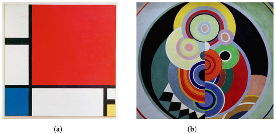
Figure 1.
Example works of abstract Cubism and Orphism. (a) Piet Mondrian, 1930: “Composition II in Red, Blue, and Yellow”; (b) Robert Delaunay, 1938: “Paris Rythme” (Photo by Jean Louis Mazieres 1938).
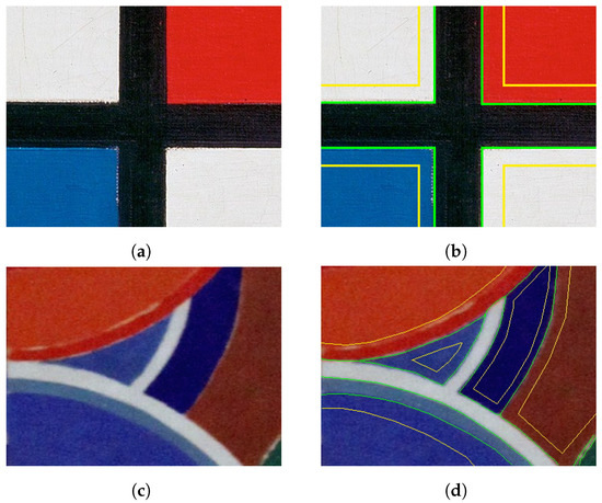
Figure 2.
Sections of Mondrians and Delaunays paintings with boundaries highlighted. (a) Section of Mondrian’s painting from Figure 1a showing an area with multiple straight region boundaries; (b) boundaries marked (green: region boundary, yellow: inside/border region); (c) section of Delaunays Painting from Figure 1b showing an area with round boundaries between regions; (d) boundaries marked as above.
These features are particularly challenging for a robotic painting system since small deviations can already ruin the overall impression. For example, if a dark stroke slightly intrudes into an adjacent light region this error is nearly impossible to recover from. If the light paint is thin, even repeated reapplication will likely not fully conceal the overpainting event. In case the light pigment is also quite opaque (e.g., Titanium White) we risk an oscillation: the imprecise brush handling which leads to the error in the first place can reoccur and move the problem into the dark area. Since the robot cannot adapt its technique on the fly, it can get suck correcting each side repeatedly. If drying times are not considered, moving over the freshly painted dark area will lead to picking up the pigment and mixing it into the light area, further escalating the error.
How do human painters solve this problem? Either they use aids, such as masking tape, to produce straight, clean lines in one go, or they rely on their painting experience to create the feature carefully. Importantly, they will switch between a mode for filling in the interior of a shape and creating the outline. In “outline mode” painters steady their hands, go slowly, and pay great attention to their brush’s trajectory. They can either draw a stroke directly to the desired edge or use multiple strokes, with each getting closer to the desired contour. The main goal of the latter strategy is error prevention, since putting in more effort to not make a mistake is often quicker than fixing it.
Since a painting robot is much more limited in error correction behavior, such as scraping off paint later, a conservative approach seems beneficial. We describe a solution in Section 3.2, which allows us to place paint without exceeding one or two constraining boundaries. Primitives for painting sharp, precise linear, and angular boundaries are generally applicable as any painting in any style might require a sharp delimitation of adjacent regions. We refer to them as constrained regions in the following. This is mirrored in the development of Purism, an art style that developed as a criticism of Cubism and stems from a return to painting objects, albeit in a Cubist-influenced style (Ball 1978). Ozefant, a main developer of the style, went on to call Cubism a “mere decorative vehicle” he compared to “carpets” (Ozefant and Corbusier 1918). The derived style focuses on still lifes, in which objects are represented as flat planes with neutral colors (Britannica 2022).
1.2. Post-Impressionism: Van Gogh and Cézanne
Post-Impressionism describes an art period between roughly 1886 to 1900 which branched off from Impressionism (Brodskaïa 2018). Impressionism is considered a reaction against a “classical” style of Greco-Latin painting in oil, choosing instead to change the choice of subjects and painting technique. Landscapes with visible strokes and intermixing colors were often used (Mauclair 2019). Post-Impressionism in turn rejects the naturalistic form of Impressionism and seeks the use of simpler colors, more visible shapes, and a more abstract representation of things (Voorhies 2004). As such, this art style is also of interest for our analysis: The complex colors and gradients used in Impressionist works are difficult to realize deliberately with a robot, and also the analysis of a work to plan painting actions is nontrivial. Visible shapes in simpler colors are more approachable.
Works by Vincent van Gogh are famous works of Post-Impressionism. His paintings are frequently used as example sources in GAN-based style-transfer, see (Gatys et al. 2016), as the overall structure is characteristic and visually defines the image. In van Gogh’s paintings, regions are not necessarily separated by color and not necessarily monochrome. Instead, regions arise from similarly oriented or shaped strokes. Borders between regions can arise from differently oriented “streams” of strokes clashing. Within a single region strokes of totally different colors can still form a coherent area, as shown in “the sower” (Figure 3). For example, the wheat field in the background is not separated from the blue foreground using a strict line, but instead, the vertically painted straws naturally distinguish themselves from the blue foreground, made up of shorter, horizontal strokes. Even regions of very similar color can be separated by structuring elements: The vertical yellow wheat strokes are distinguishable from the horizontal, but also yellow, sky (Figure 4a). Smaller elements are also paintable using structural differences, such as the legs of the titular sower, which have a blue hue similar to their local background, but as the stroke orientation follows the legs, it contrasts the field (Figure 4b).
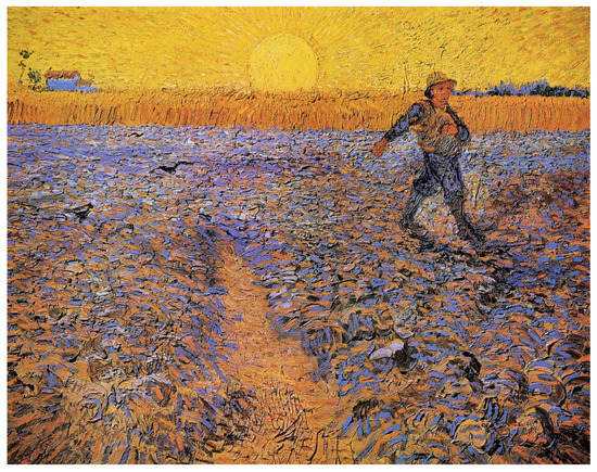
Figure 3.
“The Sower” by Vincent van Gogh (Photo by Gandalf’s Gallery 1888).
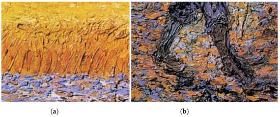
Figure 4.
Sections of “The Sower”. (a) Three structured regions with orthogonal orientations bordering each other; (b) a more complex structured region, with some boundary violations.
From these features, we can derive the need for a similar primitive in robotic painting: large-scale structures can be characterized by a general area they should cover, a structuring element, and one or more filling colors, at different densities. Their main use is for backgrounds or large objects which are not the main subject of an image. Realizing them with a purely SBR method would be tedious as the exact placement of features does not matter, but these would still cause high error values, long painting times, and likely repeated overpainting of smaller elements. Instead, we aim to implement a primitive that “roughly” paints such a region without getting stuck on unimportant details. Measuring area coverage, the density of the involved colors, and the structure overall are preferred over checking the placement of each detail. In the following, we refer to such areas as structured regions.
Finally, we observe the paintings of Paul Cézanne, specifically his landscape paintings (Figure 5). In these, we again see regions of individual colors. These are sometimes strictly delimited, with darker lines enforcing separation between roofs, corresponding to the previously discussed constrained regions. In other places, a structure is only hinted at with hatching-like structures. Elements such as trees, clouds, or boulders are represented with this technique. In doing so, Cézanne abstracts away very detail-rich areas, while still preserving the general meaning. Overall, the exact location of a hatched structure is not critical, however, the orientation and color relative to the surroundings are. As opposed to the larger structured areas of the “Sower”, we can identify substructures within a region corresponding to, for instance, a tree canopy. Figure 6b shows a section of a tree in which rough branches mesh with leave structures that are drawn as multiple rough brush motions, using different shades of green. The leaves form a glaze over the branches, giving an impression of depth. Figure 6a shows an interaction of foreground and background: the gray sky, the blue sea, and the green leaves all overlap together and give the tree transparency.
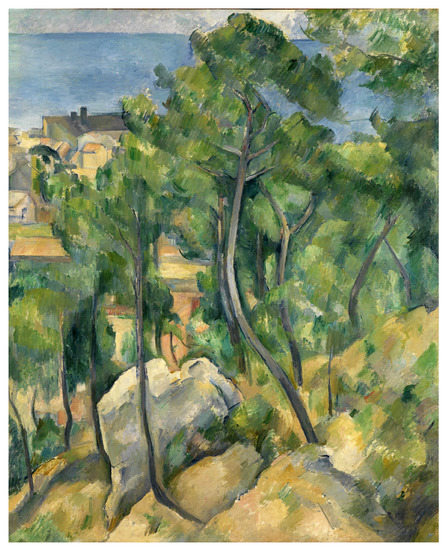
Figure 5.
View of the Sea at L’Estaque (Photo by lluisribesmateu 1969 1883–1885).
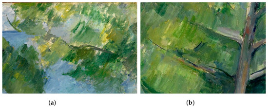
Figure 6.
Sections of “View of the Sea at L’Estaque”. (a) Part of a tree with gestural strokes; (b) sketched branch structure in a gestural tree.
To replicate these effects on a painting machine, the introduction of a gestural area is convenient. It represents the application of a known brush technique to a specified area. The program or artist planning the infill of a region can apply these to a structure to quickly achieve a visual impression. As opposed to structured regions, these are smaller primitives, usually only associated with a single, albeit complex, brush movement. It is also possible to prerecord these actions and store them for later use by a planner. By comparing elements of such a library to patches of an image a sufficiently predictable action can be selected and applied confidently.
2. Related Work
For a historical perspective on the development of painting machines, we refer to Gülzow et al. (2018). This allows us to focus on recent developments related to region-based painting and other trends in robotic painting after 2015.
Berio et al. (2016) present a method for fluid painting robot motion, which enables their robot “Baxter” to produce human-like graffiti writing. Their approach does not focus on the production of precise regions but on the creation of calligraphic movements. This approach is more low-level and uses direct motor control with custom inverse kinematics, emphasizing the motion side of the painting process. Such direct control is less conductive to precise painting, however, larger features can be realized with these methods. Their graffiti is also performed with very wide pens, which cover a significant region of canvas in a single application.
The Busker painting robot, developed by Scalera et al. (2018) has been used in multiple projects with different tools to produce paintings.
Airbrush painting is a common task for robots in car manufacturing, with specialized robots existing only for this task. These machines focus on providing a homogeneous, single-color coating for car bodies. In the arts, airbrushes can also be used but the task shifts to depositing multiple colors for image creation. For this purpose, Seriani et al. (2015) measure the paint distribution achieved by an airbrush nozzle at different distances from a canvas and use a 2D Gaussian distribution to model it. They use the distribution outline for path planning inside of polygons and consider the time spent at each location to predict paint deposition. This allows them to create grayscale reproductions of a target image. In Scalera et al. (2017) a similar approach is revisited. Airbrush painting is region based by its nature and necessitates the decomposition of an image into sprayable regions. The main limitation is the difficulty to realize small features. Sharp edges also cannot be realized without additional tools.
Busker has also been used for painting with watercolors: in a recent study, Scalera et al. use basic image analysis tools, such as Canny edge detection and Hough transform to divide an image into hatching areas. The main focus of this work is on stroke artifacts, which occur from the interaction of pigment dissolved in water, which can still move after a stroke has been placed. Inhomogeneous regions such as backruns, granulation, and edge darkening occur due to this phenomenon. The authors use their visual system to measure the reduction of pigment along a brushstroke, which allows them to terminate the stroke before pigment deposition becomes ineffective. Finally, a magnet-based system for automatic brush changing is discussed in (Scalera et al. 2019).
Beltramello et al. (2020) also use a UR-10 robot and equip it with a palette knife, in order to create paintings. Unlike most other approaches which use soft tools, this is a rare use of a rigid tool. The authors present multiple ways to create strokes with different features, depending on the application of the tool. Input images are processed from high to low frequencies, with each layer resulting in a binary mask, that is filled with hatching patterns. The tool is oriented with respect to the edges of painting regions. Furthermore, they characterize the covered area and achievable line length with the palette knife in relation to the paint angle and tool path length. While the robot has a webcam to obtain images of the canvas, its algorithm does not seem to use visual feedback during the painting process. Instead, the optical system is used to localize the painting area and to create a correspondence between the robot and canvas coordinate system.
In a recent paper, Scalera et al. (2022) use a sponge to fill in regions. They propose a contour-filling algorithm that considers the sponge’s footprint and creates paths that paint a given area without violating the defined outline. Scalera et al. use a Voronoi-based image segmentation which divides a pixel image into paintable regions. By applying image erosion, they find inner, outer, and median regions, which place different constraints onto sponge positions. The authors also present a calibration tool for the used KUKA LBR iiwa robot (see KUKA AG 2022). Their system can fill in preprocessed images in a region-based way.
Overall, multiple robotic painting systems have been developed further in recent years, all with different approaches to painting. The variety of tools and painting media shows the potential of this area of robotics and art. However, most projects are limited in accuracy due to both painting tools and media being hard to predict in their precise effects. Additionally, the main focus is on filling regions with a single color. In the following paper, we propose methods to expand robotic painting beyond these limitations, by increasing region accuracy and considering region texture.
3. Materials and Methods
For the experiments described below, we use the e-David painting robot, as described in (Gülzow et al. 2020). The machine is equipped with round nylon brushes of various sizes and uses premixed acrylic paints, which the robot picks up automatically from a palette. As a painting surface, we use acrylic paper. The methods described here are not dependent on specific painting media and can be used for other types as well.
All methods require the use of the visual feedback system, which allows image acquisition of the canvas after some brushstrokes have been executed. Feedback pictures are corrected for lens distortion to ensure a precise pixel to canvas location mapping. We also correct for lighting and color deviation using calibration targets on the canvas base. For placing brushstrokes we compute the expected width for a certain pressure level using the width-calibration method described in (Gülzow et al. 2018).
3.1. Overview of Brush Defects/Precision Limitation of Robotic Strokes
The basic action a painting robot can perform is to move a brush over a canvas, producing a stroke. While these strokes are executed precisely and can be repeated easily, they are not a fully controllable primitive.
In fact, even a straight line, seemingly a very simple stroke, is already not trivial to paint precisely with a robot. Ideally, the paint would be applied evenly around the movement path, but in reality, a multitude of effects take place due to the complex behavior of paint brushes. As the tool contacts the canvas, hairs interact with each other which can cause single bristles to detach from the main brush body and paint far away from the intended site. The paint in the brush is pushed out under compression, creating a distinctive blob and a large amount of paint is deposited. This can overshoot both an intended edge as well as a specific tone of color. As the brush is dragged over the canvas, the amount of paint deposited steadily decreases. When moving along a straight line, bristles that have spread out initially, rearrange and form a thinner stroke. In case of any direction change, the brush hairs will lag behind the tool center point (TCP) path, depositing paint offset from it. Finally, when the brush is moved away from the canvas again, the deflected bristles relax and can extend the stroke beyond the endpoint of the intended path. Figure 7 shows a stroke painted with a simple two-point trajectory which highlights these problems. The consequence for robotic painting is that if these effects are not controlled, the introduced deviations destroy small features locally and lead to a global noise, which significantly degrades the final result quality.
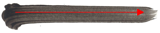
Figure 7.
A brushstroke with the two-point path the robot followed indicated. The beginning of the stroke is wider than the main body and the stroke extends beyond the expected endpoint.
Aside from instantaneous brush dynamics, the tool can bend over time. The bristles might bend permanently away from the direction of travel, which creates an offset between TCP and brush tip. This effect can immediately lead to excursions beyond a critical edge when attempting to paint it directly. Managing long-term bends such as this is very difficult to manage or simulate. Another common issue is warping of the paint surface from excessive wetting. SBR-based algorithms will tend to correct many errors around difficult features, which leads to a lot of paint being deposited and thus moisture entering the canvas area. When painting onto paper, the surface will warp with some spots rising to one or two millimeters. This immediately distorts any further brushstrokes, making the problem worse. Avoiding repeated application is important.
A more detailed description of some of the factors mentioned here can be found in (Gülzow et al. 2018). Human painters are less concerned with such details, as they can continuously improve their skill in managing brush behavior through practice and can correct errors. Robotic painters so far either rely on the repetition of a small number of well-known strokes, similar to stippling, or on reacting to errors using feedback and overpainting defects again and again (see Lindemeier et al. 2015). Stippled images forgo a lot of possible variety, while feedback-driven overpainting risks that fixing a stroke artifact with further strokes can introduce more errors that need to be fixed with yet more strokes. Convergence might not be achieved in some tricky image regions. Furthermore, the difference between a desired effect and an artifact might be dependent on image context, which makes global SBR methods difficult to apply. Attempts have been made to capture brush behavior for more specific painting approaches, like Sun et al. with their work on Callibot, a machine designed explicitly for Chinese calligraphy (Sun and Xu 2013; Sun et al. 2014). Unfortunately, this does not generalize to painting as a whole.
Our proposed solution to this issue is constrained regions, in which we isolate the predictable parts of a stroke for feature creation while hiding parts of the stroke with potential defects within an area that can be overpainted safely later.
3.2. Constrained Regions
For a constrained region we intend to place pigment on the canvas only within the given region and never exceed the boundaries. Critically, we must assume that some actions lead to almost unrecoverable errors, e.g., when a very dark stroke is erroneously placed in a very light region. However, it is possible to exploit parts of a region that are known not to represent critical features for the image and concentrate stroke beginnings and ends there. This “hides” artifacts away within a region so that they can be safely overpainted later, without risking damage to critical edges. We describe regions as general polygons which can have concave and convex regions. In concave parts, we are only required to correctly match one line of the outline of the polygon and can hide stroke beginning and end zones on the inside of the shape. Convex parts are more challenging as there is no room to hide errors there. As shown in Figure 8, we subdivide polygons into corner areas (red) and side areas (blue) depending on the local distance to one or two polygon sides.
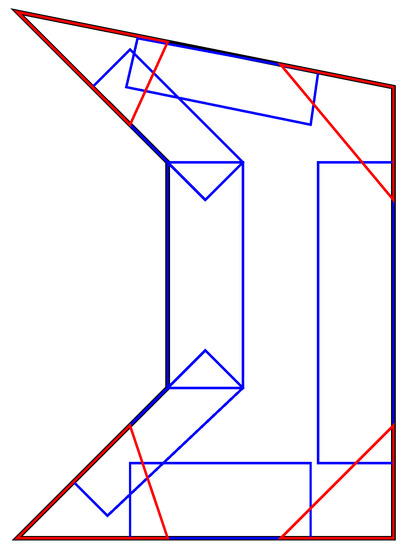
Figure 8.
A polygon with constrained regions highlighted. Red corner areas are on two sides, blue side areas are constrained on only one.
The subdivision of a polygon is based on the stroke width achievable with the current painting tool. A method to predict brush stroke width from application pressure is described in (Gülzow et al. 2018). We select a pressure one third between the minimum and maximum possible pressure for a given brush, resulting in a known stroke width w. Parameter k is user selectable and determines the resolution at which a polygon is painted. For most round brushes we use , as this produces a stroke with stable features.
In the following, we assume that all polygons which should be painted are realizable with the given tools. If the polygon contains any segments with a length less than , a warning is emitted. Additionally, if an acute corner is found, which is so narrow that most of its area is narrower than the minimum achievable stroke width, this feature is deemed unpaintable. The approach described here can detect such errors, but relies on input data which is adapted to the limitations of the current tool set.
First, convex corners are detected by measuring all internal angles of the polygon. Around such points, we draw a circle of radius . The intersection points of this circle with the two outgoing segments and the corner form a triangle, representing a corner area. Second, segments between two concave points yield rectangular side areas, which are constructed by offsetting the segment into the shape by . If this would intersect any other segments, k is reduced until this can be avoided. Third, segments with one or two ends in a corner are trimmed to the corner region and also extended into the shape. Finally, we expand all side regions by w in order to achieve some overlap and avoid gaps between strokes. No expansion is performed if this would violate an outline.
By painting both types of border elements without exceeding any edges, an inside region is established in which we can paint without needing to consider overpainting. This can be achieved with structured regions as described in Section 3.3 and is skipped for now.
3.2.1. Single-Side Constrained Regions
Single-side constrained regions (SSCR) are mostly rectangular areas that have one straight or slightly curved side which must be painted exactly. All other sides are considered to be unconstrained and may be painted over. This reduced requirement allows us to use the brush in a way that guarantees underpainting and then correcting for that brush behavior using visual feedback. If we directly painted a line along the constraining edge, variations in line thickness could cause us to exceed the edge. The bristles are not sufficiently constrained in a regular stroke. Overall bristle length however is a fixed constraint, which we can exploit for this use case. Since they are rigidly attached to the ferrule, they can only pivot around the attachment point and the brush tip must be on or within a circular arc, centered on the bristles attachment point. Thus, we apply the brush to the canvas with a sideways tilt (Figure 9), and given the brush pressure and bristle length we can compute the tip position on the arc. This adds a certain offset to our stroke, called brush tip overshoot or . We can compute this effect using the following formula for a line–circle intersection, with the circle as the swing arc of the bristles and the line the canvas1:
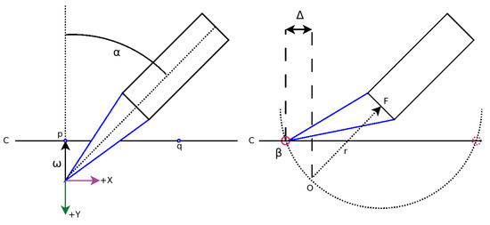
Figure 9.
Brush tip (blue) deflection along an arc when pressure is applied demonstrating brush tip overshoot. Red circles mark the found intersection points, from which we select the cone closest to the brush tip.
See Table 1 for the involved parameters.

Table 1.
Parameters for predicting brush tip deviation.
We assume the robot TCP is located at O, which we assume to be the origin for the following computations. First, we find the brush hair fulcrum point from polar coordinates:
Since we are only looking at 2D deflection, the canvas C is a line parallel to the X-axis, from which we select two points:
We use p and q to calculate the determinant D:
In Equation (5) will always be zero for our choice of p and q. However, if the canvas is at an angle this is no longer the case. Hence we include in the following equations. We now obtain the intersection points and of the brush arc with the canvas as:
From which we pick the final closest to the origin (lying in the tip of the brush) from which we decide . Knowing enables us to directly paint along a constraining line and to realize said feature with much more precision than just painting without prior knowledge. However, other sources of error exist, which are harder to compute and require the use of visual feedback to control. While applying the brush to the canvas causes it to slip forwards by the computed amount, sideways movement causes the brush to bend away from the goal edge. As this effect is less uniform, we use the following method to iteratively approach a target line:
First, a stroke is placed in parallel to the target line, offset by , where is some user-defined safety distance. After a stroke has been placed, an image is taken and we compare it to the intended color of the feature. This is done by converting the image to LAB color space (see Schanda 2007) and then subtracting the target color from the image. Since we know the intended location and the location of the initial stroke we can detect a discontinuity in the difference image by scanning between the goal and stroke. We use the measured distance to move the next stroke movement closer to the target line and repeat this process until the target is reached within a certain tolerance. Figure 10 shows a sketch of this strategy as well as a sequence of SSCR strokes as executed by the robot. By extending the movement beyond the unconstrained sides of the SSCR we hide the effects of extended or shortened stroke ends away from the critical feature. We also move the brush up and down the constraining edge multiple times to even out paint deposition artifacts.
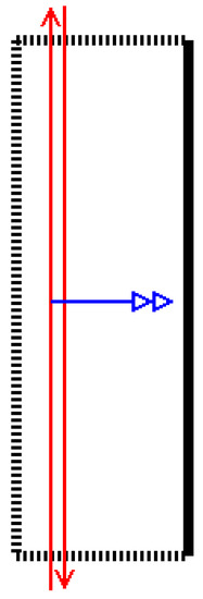
Figure 10.
Concept and effect of SSCR painting: the target line is slowly approached with alternating strokes. We begin at a safe distance from the target line and take feedback images after each stroke. Once the line is reached by the strokes, the process terminates and the edge is realized.
Overall, we can move along the intended constraint line and be sure we will never overpaint it. Usable tilts for brushes have been found to lie between and . Results can be seen in Figure 11.
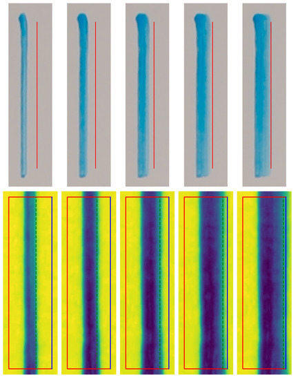
Figure 11.
Progression of the iterative SSCR process. Top row: color images of the stroke sequence. Bottom row: difference images with yellow indicating high difference and blue low difference. The box is the SSCR with the blue line marking the constraining side. The green dashed line is the edge detected by the system.
3.2.2. Two-Side Constrained Regions
SSCRs can be used to paint the exterior sides of polygons. However, they are insufficient to realize the corners of any convex feature shape, since in that location two edges must meet at a single point. Any lateral overpainting of the SSCR would destroy the adjacent edge, so it is insufficient to just place two SSCRs over each other. We also define two-side constrained regions (TSCR) which can realize a corner feature by placing strokes aligned with both. Corner features are especially critical since any overpainting or misplacement ruins a salient point of the shape. At the same time, controlling the brush with respect to two constraining edges is difficult. We implement a feedback-based strategy in two steps, shown in Figure 12.
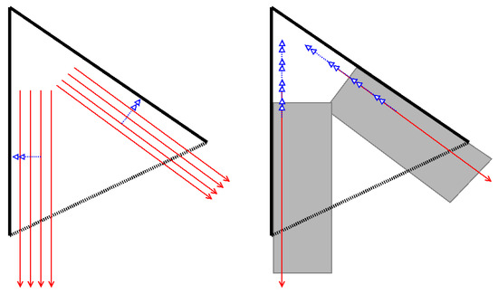
Figure 12.
Strategy for the realization of corners. Left: in the first phase, move the strokes closer to the sides until we find a working suitable distance. Right: in the second phase, the found strokes are moved towards the tip until the region is properly filled. The gray area has already been covered in phase 1.
First, we create a stroke from each constraining side and offset it towards the inside of the shape and shift it towards the unconstrained side. This allows us to paint two strokes that are guaranteed to lie within the TSCR but do not yet touch the outer edges. In the first phase after both strokes are created a feedback image is taken and the distance of the resulting strokes to the side is measured. If distance remains to the outside edge, we move the next planned stroke towards the edge until it is reached (see steps 1–3 in Figure 13). Once the outside edge has been reached, the stroke is moved in parallel to the edge in by half of the expected stroke width while the distance to the tip is measured (steps 4 and 5 in Figure 13). Once the tip is sufficiently covered the TSCR is considered done as a safe inner region for filling has been established. The final strokes are stored as a limit for further strokes in the region. Figure 14 shows the first step and the final result in more detail.
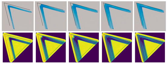
Figure 13.
TSCR paint progression shown in robot feedback images. Upper row: raw feedback images with a black line added to indicate the target corner.
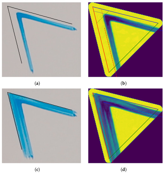
Figure 14.
Progression of painting a corner using a TSCR. The left column shows the feedback images and the right column the difference images with measured corners indicated. The first two figures show the canvas state after the first step while the last two are taken five strokes later once the process had terminated. Note how the placed strokes were planned equidistant to the constraining sides, but the placed strokes are much closer on the right. This shows that brush deviation must be handled via optical feedback. (a) Initial painting of a corner with different distances despite paths being planned equidistant from goal sides; (b) measurement of initial strokes: the dotted lines represent the distance from the left edge (red), right edge (blue), and the tip (green). The dashed lines show the next planned corrective strokes; (c) finished corner with minimal overpainting of the target line. Only the unconstrained side is violated; (d) the final result: the painted regions are found to coincide with the target edges. The tip has been fully realized. This terminated the corner painting procedure.
As with SSCRs we also tilt the brush, but towards the single unconstrained edge. This avoids artifacts in the first part of a stroke, which are critical to forming the corner. We also modulate brush sideways tilt towards the inside of the TSCR, away from the outer edge. This is analogous to the SSCR and avoids brush expansion to violate the constraining corner. In this compound angle, we again compensate for brush tip overshoot and move the brush from the tip to the unconstrained edge, along the constraining edges.
After an SSCR or TSCR has been correctly realized, the resulting final strokes are partially reusable in similar features. If the tool itself, the tool orientation, the paint medium, and the application pressure remain constant, repeating the strokes will also result in an approximate copy of the created feature. Storing these results allows us to reuse them later for similar features in other paintings. Over time, this allows the robot to build a library of techniques, which speeds up the painting process and allows for more analysis of brush behavior. This, however, limits the accuracy of the feature, since there is no chance to react to certain errors, like brush tip drift, paint changing consistency in the reservoir, or canvas warping (if painting on paper for example).
To realize a whole polygon, SSCRs and TSCRs can be painted in any order, since no constrained side will ever be overpainted and adjacent constraining lines are always parts of the same original segment. In our approach, we paint corners before the sides, as this gives a better visual indication of where a shape will be located during the painting process.
3.3. Structured Regions
For a structured region (SR), we restrict the set of allowed brush movements that are used to cover a canvas area. As described in Section 1.2, the goal of this method is to enable the painting system to create visual impressions not only via color application but through stroke structure. Applying normal stroke-based rendering techniques for this purpose would not be appropriate, since they rely on repeated overpainting for error minimization. This would diminish structure effects since at some point a canvas area is saturated with paint and additional brush applications simply even out the distribution.
Given some structuring element, such as a direction vector, we orient the movements and through repetition cover the region. With a single color, the brush dynamics create a visible structure, which then characterizes the area. Additionally, we can allow multiple colors, similar to the previously discussed van Gogh painting “The Sower”.
For structured regions, we assume the edges to be unconstrained since altering brush movements to avoid outer edges would change the goal structure. Instead, we assume strokes may be painted slightly over the border of the given region. Such an effect can be beneficial, e.g., in the case of a field of grass overlapping into the sky at the horizon. Furthermore, a structured region can be combined with an outline of constrained regions to achieve more precision at the expense of a homogeneous structure.
An underlying structuring field is used to guide stroke placement. In the simplest case, this can just be a constant vector for an entire shape, like in the case of a corn field. Other potential metrics include painting along the distance transform (DST) gradient or the edge tangent field of a template image within the region being painted.
To assess the painting progress from feedback, we determine the overall coverage, average color, density of strokes, and texture structure. The average color is simply measured by averaging all feedback pixels of the region. Coverage density can be estimated via background subtraction: if the background is covered to the desired degree, sufficient coverage has been achieved. Multicolor regions require the uniform presence of all involved colors. We measure the frequency of each color and identify subregions with lower concentrations. There, strokes of the missing color are placed. The texture of a region is assessed from the response of Gabor filters, as described in (Fogel and Sagi 1989). By orienting the filter according to the local structure field and selecting the frequency to correspond to the stroke width, we detect the presence of structured strokes. In case the orientation is erroneous or the area is too homogeneous, we place further strokes on top.
3.4. Gestural Regions
As seen in the works of Cezanne, some parts of an image need not exactly match a real subject but hinting at their structure is sufficient for an artwork. In the same spirit, we use predefined complex stroke movements and apply them to a region to produce a gestural effect, corresponding to their structure. By overlaying multiple of these in different colors, a complex region is achieved. Unlike the previously discussed techniques where brush movements consist usually of a more or less linear motion, the complex movements used for gestural movements are longer, can self-overlap, and are not designed to minimize brush dynamics. For example, in a zigzag movement pattern brush deflection changes significantly at the point where the stroke path changes direction to the point of almost reversing. If the pattern self-overlaps, paint that has just been deposited might be moved again in the same movement. Both these effects can be useful for achieving certain visual effects but are difficult to control exactly. Hence treating them as a special case in painting allows the combination of precise and imprecise elements in robotic painting.
We implement a side-to-side scribbling motion, dabbing of the brush, and a swirling brush action, which are performed in a given gestural region. These can then be rotated, scaled, and placed to approximate an image element. For the realization of a gestural region, we allow overpainting of the region boundaries and focus instead on area coverage. This is achieved by computing the initial movement pattern for the given shape and using visual feedback to detect uncovered areas. Color is reapplied in these areas until the entire structure has been realized. While this is not a major novelty in robotic painting, the introduction of this primitive gives a user of the painting robot the ability to realize certain structures more easily. Instead of planning individual strokes, the painting system can take over parts of the planning process.
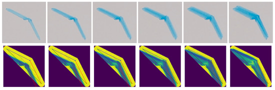
Figure 15 shows a simple tree painted with gestural regions: the paint plan consists simply of branches and boxes representing areas covered by leaves (Figure 15a). These are then replaced by zigzag lines with some jitter added (Figure 15b,c). Variations of the tree are produced by swapping out the gesture, for example in Figure 15d a spiral movement is used instead of a zigzag.
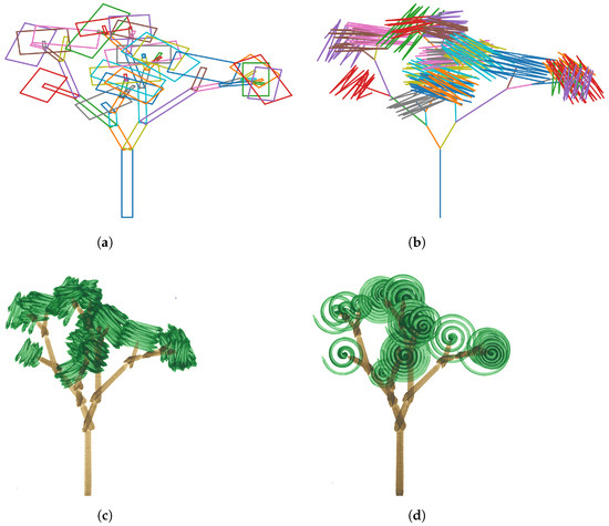
Figure 15.
An example of how gestural regions can be used to realize variations of a tree: a paint plan is generated from a simple procedural model which results in a set of branches and leaf patches (a). These are then translated into a gestural stroke (b), which in this case is a zigzag. When realized on the machine, this leads to some regions being quickly covered with paint, without the need for feedback (c). Since the initial plan is kept abstract, and regions are labeled as either branch or leaf, it is easy to swap out gestures for others (d).
4. Results
With the implementation of constrained regions, the e-David painting system has gained the ability to predictably produce accurate outlines for arbitrary polygons. Except for extreme angles, any such feature can be realized. The initially slow painting time can be compensated by storing the results and repeating them directly for similar regions. Thanks to the continuous measurement we can approximate corners and edges with a precision of , independent of the tool, paint medium, or location on the canvas. If a faster painting result is desired, the formula for tip deviation presented in Section 3.2 can be used, which allows planning a brush movement directly. While some error must be expected, this is still accurate to . See Table 2 for an overview of the achieved precision in the presented TSCRs.
Table 2.
Achieved precision in the realization of the TSCRs shown in previous figures. Negative values indicate the measured edge lies within the constrained region, while positive values show overpainting outside of the region. The resolution of the feedback system is 0.3 mm per pixel.
Figure 13 shows the output of a TSCR used to paint a corner with a angle. The initial strokes are painted well clear of the border (Figure 14a). Here we can already see that the initial strokes are not equally spaced to the goal corners, as the upper one is closer. The deviation is due to the brush being deformed by a previous stroke in this case, which is not predictable. Due to exactly this effect, an iterative approach is needed. The distance to the sides and tip are then measured for the newly created strokes (Figure 14b and the corresponding offset is applied). By repeating this until the stokes are placed exactly along the goal edges, we achieve the result seen in Figure 14c. The corners and tip are filled precisely and the robot stops before any overpainting occurs. Figure 14d shows the final error image.
We have also tested the applicability of this method for , , and corners, as can be seen in Figure 16, Figure 17 and Figure 18, respectively. In all cases, convergence is achieved and the desired angle is produced at the required location. All shown images are taken directly from the robot’s visual feedback system. The resolution achieved is 1 pixel per .
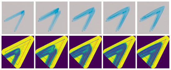
Figure 16.
TSCR paint progression for a 30-degree corner. More tolerance is given at the tip since the tool cannot reach into it fully without violating the other constraining side. Top row: feedback images with no annotation. Bottom row: difference images with annotated goal and measurement lines. In the first two images, the strokes are moved from the inside towards the goal lines. Once these have been reached, the strokes are moved towards the tip, which fills it in.
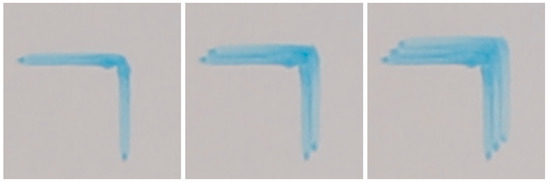
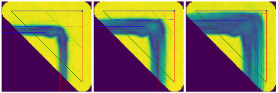
Figure 17.
TSCR paint progression for a 90-degree corner. Similar to Figure 16 a corner is filled in by moving strokes towards the sides and then into the corners. Shown here are iteration steps 1, 3, and 5 of the realization process.
A drawback is that the tips of two-sided constrained regions do not come to a perfectly sharp tip, but even for humans such features are not always realizable. Furthermore, most painting tasks do not require such features but only need the impression of a pointy outline.
Figure 19 shows the progress a structured region. A region is covered with a single pigment and a horizontal structure. Within three iterations we achieve full coverage of the intended region (red box). Due to the brush’s texture, a structure is achieved in the desired direction. The outline of the region is not considered by this approach, but by outlining it with constrained regions first, a sharp corner can be achieved. Experiments have shown that using a single attempt to realize such a region without feedback is not guaranteed to work since the required stroke density to achieve a guaranteed cover is very high. Despite this, brush behavior might lead to some uncovered areas. From Figure 19b,c we can see how remaining holes are detected and filled in. Figure 20 shows a small example painting where two structured regions form a simple landscape: The sky consists of horizontal strokes with larger white strokes added as cloud details. The grass is made up of shorter vertical strokes and red dots are added as details. The paint plan for this image only consists of two rectangles with the appropriate information.
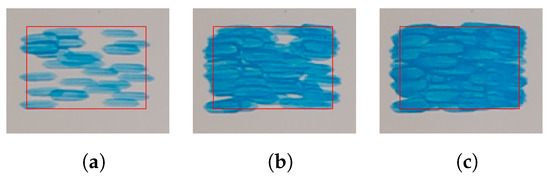
Figure 19.
Execution of a monochrome structured region with a horizontal structure vector. The target area is shown with a red box and covered within three iteration steps. (a) Initial stroke set; (b) first feedback step; (c) second feedback step.
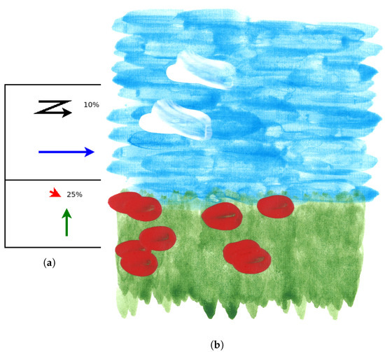
Figure 20.
A simple landscape painted with structured regions. It consists of two rectangular areas, with different attached attributes. The sky consists of a blue coverage with horizontal orientation with an added white zigzag stroke covering of the area. The grass is made up of vertically oriented green strokes, which are also shorter. Additionally, a coverage with simple red dots as flowers is layered on top. (a) Sketch of the structured region input: each region is defined with a primary structuring member and some additional elements to be painted on top with a specified density; (b) the painting created from the given input data.
Figure 15 shows a basic fractal tree, painted using gestural techniques. While from a technical perspective this is not very noteworthy, offering such primitives to users of robotic painting systems is important. First, more abstract handling of the painting process hides details of SBR from users. Secondly, the ability to give more vague instructions over always requiring precise stroke commands makes the system more approachable and replicates some of the vagueness inherent to painting as discussed in Section 1.1. Finally, it allows for simplified automatic paint planning, as unimportant regions can be marked for rough gestural infill. Generating synthetic images, such as the shown trees also becomes easier. In this case, a simple fractal tree was generated as a set of boxes representing foliage and branches (Figure 15a). Foliage boxes were replaced with zigzag-like strokes, resembling those of Cézanne in Figure 5. The resulting leave structure in Figure 15c is somewhat similar. Figure 15d shows the same tree structure painted with spiral gestures instead of zigzags.
5. Discussion
The initial idea was to move robotic painting closer to how humans work by moving to different types of paintable regions instead of strokes as the basic building block of an image. We have described three concrete methods to achieve this and show their applicability in different situations. These higher-level constructs are a new approach in this field and allow robotic painting systems to become more usable, efficient, and human-like in their results.
We have demonstrated a working implementation of constrained regions which are realized using information about the used paint brush and visual feedback. The process allows for the precise realization of corners and edges, which can be used to create polygonal structures in painted images. The locally iterative process which focuses on direct measurement of the effect of previous actions is novel in robotic painting. Furthermore, since brushstrokes are guaranteed to not violate adjacent regions, the iteration stop for the feedback process is well defined. The main limitation of this method is that small details are not achievable, since some space is required to place initial strokes. This must be solved separately by planning individual strokes. Furthermore, the realized features usually show the brush stroke structure that was used during the feedback process, which might not be suitable for all use cases. Despite this, constrained regions are a major step toward imitating human pictorial rendering techniques in robotic painting.
Our implementation of structured regions also follows this direction: traditional SBR methods would struggle with mixed areas like in Figure 4a. The optimization for an exact color match causes repeated overpainting, leading to a more homogeneous, unstructured area. Instead of focusing on coverage and overall distribution, we avoid this trap by painting only uncovered or insufficiently colored areas within a structured region. This also leads to improved convergence, since the system cannot get stuck in a loop where a feature is painted and overpainted again when adjacent colors are reapplied over each other. This occurred in previous e-David methods (see Lindemeier et al. 2015). Structured regions are again a novel concept in robotic painting as they allow a more error-tolerant style in places where an exact match to a template is not as important. The inherent drawback of this method is that a structured region cannot exactly stay within its bounds, so either some over- or underpainting of region borders must be tolerated. A combination with constrained regions placed around a structured one could be a solution in some cases.
We also introduced gestural regions as a means to quickly and roughly cover some areas with paint. We derived these from the observation that human painters tend to use rapid but coarse brush movements in areas of a painting where precision is not the main concern. The novelty of this approach lies in the use of an explicit region type for this, which benefits the planning process. Furthermore, since gestural regions are defined by their type of movement, it is possible to use interchangeable movements for varied results. Additionally, by using predefined movements which are known to be executable by a given painting machine, we can avoid stalling the machine through commands it is not able to execute, e.g., when they are limited by point density or the speed of direction changes. The limitations of gestural regions are of course their imprecise nature and lack of feedback metrics.
On the input and image composition side of a robotic paint system, regions provide the main advantage of improving planability. While in SBR the image emerges from a sum of strokes globally, the image is only finished after fully converging. When this occurs is unclear, since the noisy painting process can require going back to previously painted locations at any time. In region-based painting, a finished region does not change after completion and the criterion for said completion can be stated more explicitly.
On the output/production side of the painting system, we are now able to achieve higher quality. Constrained regions lead to increased painting precision, which many SBR-based systems have previously not been able to achieve. The ability to reliably create precise edges and corners avoids potentially uncorrectable errors which can degrade entire paintings. A secondary effect is the possibility to reuse previous painting results in a knowledge base. Placing a single stroke on some unknown background in SRB-type paintings is hard to predict and a recording is of limited use. Recording a region painted onto a blank surface with defined actions can be reused since outside effects are minimized.
The main drawback of region-based methods is that we require a segmentation method to determine paintable regions. The quality of our painting result depends on the quality of the found regions, which can be a tricky problem to solve. SBR methods on the other hand can directly work with pixel images.
6. Conclusions
In this paper, we presented multiple new approaches to robotic painting. First, the computation of brush slip based on brush hair length gives an upper bound for where a given brush application will place a stroke edge on a canvas. This is a good prior for more accurate painting. Since a complete simulation of brush physics is an extremely involved task (see Baxter and Lin 2004), using an approximation for certain aspects of brush dynamics allows us to slowly improve planning for physical painting tasks.
Second, the introduction of iteratively painted constrained regions represents a new approach to robotic painting. Our method mimics human behavior more closely, where a painter finishes an artwork region by region. We can subdivide polygons into SSRCs and TSCRs and realize them individually. Our method uses optical feedback to achieve precision within 1mm. Using constrained regions in images makes it possible to reliably paint clear edges and corners.
Third, structured regions offer an efficient way to fill in certain areas. As we have shown in Section 1.2, painted areas defined by their structure or color distribution are common in human painting. For these preserving exact edges is not relevant, as structural differences can serve to indicate borders. However, preserving the structured visual impression is not usually considered in previous methods. Our approach is structure-aware and allows the realization of these areas.
Constrained and structured regions also introduce visual feedback with frame-to-frame coherence in robotic painting, which thus far had not been used: since only a limited set of actions is used in a know region it is possible to judge the effect of single actions taken in the region, such as the progress towards realizing a line or corner. Our system can measure the achieved distance to a constraining line before and after an action, which can be used to paint future lines more directly.
Finally, gestural regions are a simple but effective method to realize certain areas in a more approximate manner. It mimics human behavior to use rough, semi-random scribbles to fill in an area of lower importance to a painting. Implementing this in robotic painting allows us to paint areas of different importance in different ways, by placing constrained or structured regions on important features, while less relevant objects are reduced to a few gestural regions. This reduces paint times, makes planning simpler, and avoids that the system spends a lot of time on an unimportant but perhaps salient feature.
Overall we introduced three new principles which can be used for better motion planning in robotic painting.
7. Future Work
To maximize the use of regions as primitives in robotic painting, the next research step must be the development of a planning tool, which automatically translates input images into a set of such regions. This will allow our approach to be as generally applicable as traditional SBR methods. Especially with the recent developments in AI-generated art, in which pretrained networks produce pixel images that look like abstract art (see Elgammal et al. 2017) or agents which translate text prompts into plausible images (see “Dall-E” or Ramesh et al. (2022)) this would allow for end-to-end machine art.
Additionally, classification of regions from semantics and structural hints would significantly improve painting quality: different objects might have similar colors, such as a blue-hulled ship on the water. Such features could be contrast-enhanced or painted with different structures to allow for a distinction. Identifying and replicating structural differences, like in all-green tree structures goes in a similar direction.
On an artisanal level, we intend to include more considerations about tool effects into the paint plan and also add a temporal component to watch for drying times. Painting next to dries areas will keep region boundaries crisp, while deliberately painting onto wet regions will allow on-canvas paint mixing or color redistribution. Furthermore, the plan should include washing the brush after potentially contaminating it in a wet area.
The methods to realize TSCRs and SSRCs presented in this paper are quite specific to the given task. Finding a more general solution to such action planning would be beneficial to expanding the capabilities of the painting system and making it easier to adapt to other aspects of painting.
Finally, the data we accumulate from the feedback of isolated regions could be used by searching for areas in new images which are similar to previously painted features. This would allow us to build a knowledge database over time.
Author Contributions
Conceptualization, methodology, software, investigation and writing—original draft preparation, J.M.G.; writing—review and editing, supervision, project administration, O.D. All authors have read and agreed to the published version of the manuscript.
Funding
This research received no external funding.
Institutional Review Board Statement
Not applicable.
Informed Consent Statement
Not applicable.
Data Availability Statement
Not applicable.
Acknowledgments
We thank Antonin Sulc for proofreading the draft for this paper.
Conflicts of Interest
The authors declare no conflict of interest.
Abbreviations
The following abbreviations are used in this manuscript:
| TCP | Tool Center Point |
| SBR | Stroke-Based Rendering |
| SSCR | Single-Side Constrained Region |
| TSCR | Two-Side Constrained Region |
Appendix A
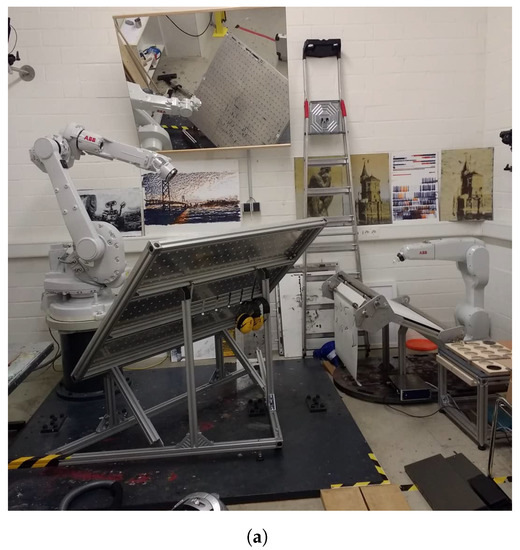
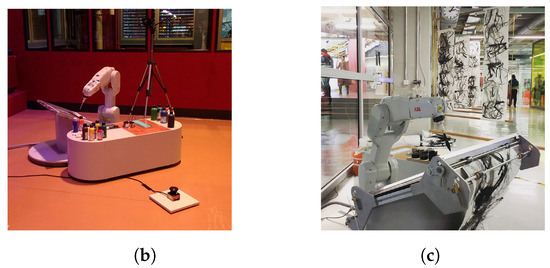
Figure A1.
Images of our robot system in various settings. (a) The robotics lab with both robots in use for the e-David system (ABB IRB 1660ID left, ABB IRB 1200 right); (b) e-David painting during an exhibition in Zürich; (c) e-David painting during an exhibition in Konstanz.
Note
| 1 | The formula for the line–circle intersection used in Equations (6)–(9) has been taken from (Rhoad et al. 1991). |
References
- Ball, Susan L. 1978. Ozenfant and Purism: The Evolution of a Style, 1915–1930. Ph.D. thesis, Yale University, Yale, CT, USA. [Google Scholar]
- Baxter, William V., and Ming C. Lin. 2004. A versatile interactive 3D brush model. Paper presented at 12th Pacific Conference on Computer Graphics and Applications, 2004. PG 2004. Proceedings, Seoul, Korea, October 6–8; pp. 319–28. [Google Scholar]
- Beltramello, Andrea, Lorenzo Scalera, Stefano Seriani, and Paolo Gallina. 2020. Artistic robotic painting using the palette knife technique. Robotics 9: 15. [Google Scholar] [CrossRef]
- Berio, Daniel, Sylvain Calinon, and Frederic Fol Leymarie. 2016. Learning dynamic graffiti strokes with a compliant robot. Paper presented at 2016 IEEE/RSJ International Conference on Intelligent Robots and Systems (IROS), Daejeon, Korea, October 9–14; pp. 3981–86. [Google Scholar]
- Britannica (The Editors of Encyclopaedia Britannica). 2022. Amédée Ozenfant. Available online: https://www.britannica.com/biography/Amedee-Ozenfant (accessed on 16 May 2022).
- Brodskaïa, Nathalia. 2018. Post-Impressionism. New York: Parkstone International. [Google Scholar]
- Chipp, Herschel B. 1958. Orphism and color theory. The Art Bulletin 40: 55–63. [Google Scholar] [CrossRef]
- Deussen, Oliver, Thomas Lindemeier, Sören Pirk, and Mark Tautzenberger. 2012. Feedback-Guided Stroke Placement for a Painting Machine. Eighth Annual Symposium on Computational Aesthetics in Graphics, Visualization, and Imaging. Aire-la-Ville: Eurographics Association, pp. 25–33. ISBN 978-1-4503-1584-5. Available online: http://kops.uni-konstanz.de/handle/123456789/23636 (accessed on 27 April 2022). [CrossRef]
- Elgammal, Ahmed, Bingchen Liu, Mohamed Elhoseiny, and Marian Mazzone. 2017. Can: Creative Adversarial Networks, Generating “Art” by Learning about Styles and Deviating from Style Norms. arXiv arXiv:1706.07068. [Google Scholar]
- Fogel, Itzhak, and Dov Sagi. 1989. Gabor filters as texture discriminator. Biological Cybernetics 61: 103–13. [Google Scholar] [CrossRef]
- Ganteführer-Trier, Anne. 2004. Cubism. Cologne: Taschen. [Google Scholar]
- Gatys, Leon A., Alexander S. Ecker, and Matthias Bethge. 2016. Image style transfer using convolutional neural networks. Paper presented at IEEE Conference on Computer Vision and Pattern Recognition, Las Vegas, NV, USA, June 27–30; pp. 2414–23. [Google Scholar]
- Grauer, Victor A. 1993. Toward a unified theory of the arts. Semiotica—Journal of the International Association for Semiotic Studies 94: 233–52. [Google Scholar] [CrossRef]
- Gülzow, Jörg Marvin, Liat Grayver, and Oliver Deussen. 2018. Self-improving robotic brushstroke replication. Arts 7: 84. [Google Scholar] [CrossRef]
- Gülzow, Jörg Marvin, Patrick Paetzold, and Oliver Deussen. 2020. Recent developments regarding painting robots for research in automatic painting, artificial creativity, and machine learning. Applied Sciences 10: 3396. [Google Scholar] [CrossRef]
- Hertzmann, Aaron. 1998. Painterly rendering with curved brush strokes of multiple sizes. Paper presented at 25th Annual Conference on Computer Graphics and Interactive Techniques, New York, NY, USA, July 19–24; pp. 453–60. [Google Scholar]
- Hiller, Stefan, Heino Hellwig, and Oliver Deussen. 2003. Beyond stippling—Methods for distributing objects on the plane. In Computer Graphics Forum. Oxford: Blackwell Publishing Online Library, vol. 22, pp. 515–22. [Google Scholar]
- KUKA AG. 2022. Lbr Iiwa Product Page. Available online: https://www.kuka.com/en-de/products/robot-systems/industrial-robots/lbr-iiwa (accessed on 27 April 2022).
- Lindemeier, Thomas, Jens Metzner, Lena Pollak, and Oliver Deussen. 2015. Hardware-based non-photorealistic rendering using a painting robot. In Computer Graphics Forum. Hoboken: Wiley Online Library, vol. 34, pp. 311–23. [Google Scholar]
- Lloyd-Davies, Virginia. 2019. Sumi-e Painting. Laguna Beach: Walter Foster Publishing. [Google Scholar]
- Mauclair, Camille. 2019. The French Impressionists (1860–1900). Glasgow: Good Press. [Google Scholar]
- Merriam-Webster. 2022. Painting. Merriam-Webster.com Dictionary. Available online: https://www.merriam-webster.com/dictionary/paint (accessed on 13 May 2022).
- Ning, Xie, Hamid Laga, Suguru Saito, and Masayuki Nakajima. 2011. Contour-driven sumi-e rendering of real photos. Computers & Graphics 35: 122–34. [Google Scholar]
- Ozenfant, Amédée, and Le Corbusier. 1918. Après le Cubisme. Paris: Éditions des Commentaires, vol. 1, Available online: https://www.britannica.com/biography/Amedee-Ozenfant (accessed on 16 May 2022).
- Parks, John A. 2014. Universal Principles of Art: 100 Key Concepts for Understanding, Analyzing, and Practicing Art. Beverly: Rockport Publishers. [Google Scholar]
- Photo by Gandalf’s Gallery. 1888. “The Sower” by Vincent van Gogh. Available online: https://www.flickr.com/photos/45482849@N03/6794532390 (accessed on 27 April 2022).
- Photo by Jean Louis Mazieres. 1938. “Paris Rythme” by Robert Delaunay. Available online: https://www.flickr.com/photos/79505738@N03/49308833571 (accessed on 27 April 2022).
- Photo by lluisribesmateu 1969. 1883–1885. “View of the Sea at l’Éstaque” by Paul Cézanne. Available online: https://www.flickr.com/photos/98216234@N08/49095670981 (accessed on 27 April 2022).
- Ramesh, Aditya, Prafulla Dhariwal, Alex Nichol, Casey Chu, and Mark Chen. 2022. Hierarchical Text-Conditional Image Generation with Clip Latents. arXiv arXiv:2204.06125. [Google Scholar]
- Rhoad, Richard, George Milauskas, and Robert Whipple. 1991. Geometry for Enjoyment and Challenge, rev. ed. Evanston: McDougal, Littell & Company. [Google Scholar]
- Scalera, Lorenzo, Enrico Mazzon, Paolo Gallina, and Alessandro Gasparetto. 2017. Airbrush robotic painting system: Experimental validation of a colour spray model. In International Conference on Robotics in Alpe-Adria Danube Region. Cham: Springer, pp. 549–56. [Google Scholar]
- Scalera, Lorenzo, Giona Canever, Stefano Seriani, Alessandro Gasparetto, and Paolo Gallina. 2022. Robotic sponge and watercolor painting based on image-processing and contour-filling algorithms. Actuators 11: 62. [Google Scholar] [CrossRef]
- Scalera, Lorenzo, Stefano Seriani, Alessandro Gasparetto, and Paolo Gallina. 2018. Busker robot: A robotic painting system for rendering images into watercolour artworks. In IFToMM Symposium on Mechanism Design for Robotics. Cham: Springer, pp. 1–8. [Google Scholar]
- Scalera, Lorenzo, Stefano Seriani, Alessandro Gasparetto, and Paolo Gallina. 2019. Watercolour robotic painting: A novel automatic system for artistic rendering. Journal of Intelligent & Robotic Systems 95: 871–86. [Google Scholar]
- Schanda, Janos. 2007. Colorimetry: Understanding the CIE System. Hoboken: John Wiley & Sons, pp. 25–78. [Google Scholar]
- Seriani, Stefano, Alessio Cortellessa, Sandro Belfio, Marco Sortino, Giovanni Totis, and Paolo Gallina. 2015. Automatic path-planning algorithm for realistic decorative robotic painting. Automation in Construction 56: 67–75. [Google Scholar] [CrossRef]
- Sun, Yuandong, and Yangsheng Xu. 2013. A calligraphy robot—Callibot: Design, analysis and applications. Paper presented at 2013 IEEE International Conference on Robotics and Biomimetics (ROBIO), Shenzhen, China, December 12–14; pp. 185–90. [Google Scholar]
- Sun, Yuandong, Huihuan Qian, and Yangsheng Xu. 2014. Robot learns chinese calligraphy from demonstrations. Paper presented at 2014 IEEE/RSJ International Conference on Intelligent Robots and Systems, Chicago, IL, USA, September 14–18; pp. 4408–13. [Google Scholar]
- van Arman, Pindar. 2020. Cloud Painter. Available online: https://www.cloudpainter.com (accessed on 15 June 2022).
- Voorhies, James. 2004. Post-impressionism. The Metropolitan Museum of Art. Available online: https://www.metmuseum.org/toah/hd/poim/hd_poim.htm (accessed on 30 May 2022).
- Weman, Klas. 2011. Welding Processes Handbook. Amsterdam: Elsevier. [Google Scholar]
Publisher’s Note: MDPI stays neutral with regard to jurisdictional claims in published maps and institutional affiliations. |
© 2022 by the authors. Licensee MDPI, Basel, Switzerland. This article is an open access article distributed under the terms and conditions of the Creative Commons Attribution (CC BY) license (https://creativecommons.org/licenses/by/4.0/).