SpArcFiRe: Enhancing Spiral Galaxy Recognition Using Arm Analysis and Random Forests

Abstract
1. Introduction
1.1. Motivation
1.2. Related Work
- We would prefer a system with parameters that are understood and can be modified by professional astronomers, and decision trees seem better suited to this task.
- Decision trees can be used to measure the quality of features3 used to make a decision and thus are more suitable for our goals in this paper. This is not the case for Deep Neural Networks, which do not yet easily provide a similar measure of feature quality.
- The most damning criticism against neural networks is that they cannot explain their reasoning to us. In particular, the way they make their decisions is not well understood, and research to better understand this issue is still in its infancy [30,31]. In short, we cannot learn from what they have learned, or learn from how they make their decisions, because a neural net is a near-complete “black box”. This is an absolutely critical disadvantage to a scientist who wants to know “why?” The goal of science is to understand, and a black box that cannot explain its rationale cannot provide us with new understanding.
1.3. Regression, Not Classification, Because Galaxy Morphology Is Continuous, Not Discrete
2. Methods
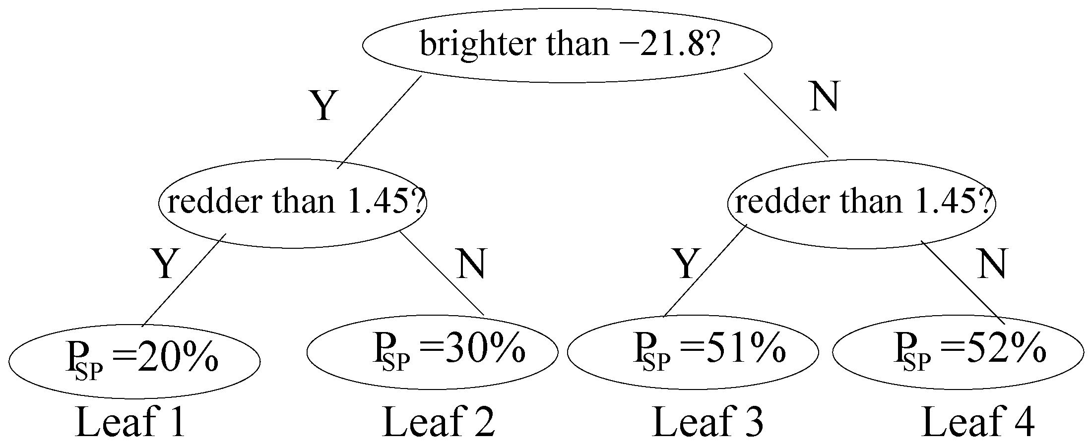
- Compute the mean magnitudes for spirals and ellipticals, respectively.
- Compute the mean colors for spirals and ellipticals, respectively.
- Compute a threshold color intended to separate spirals from ellipticals; we will simply use the midpoint .
- Similarly, compute a threshold magnitude .
- Now, for each galaxy, first ask which side of the threshold its color is on, and then ask which side of the threshold its magnitude is on.
- This bins each galaxy into one of four leaf nodes, as in Figure 2.
3. Results
3.1. Features, Trees, and Forests
3.2. Adding SpArcFiRe Features
3.3. Feature Quality
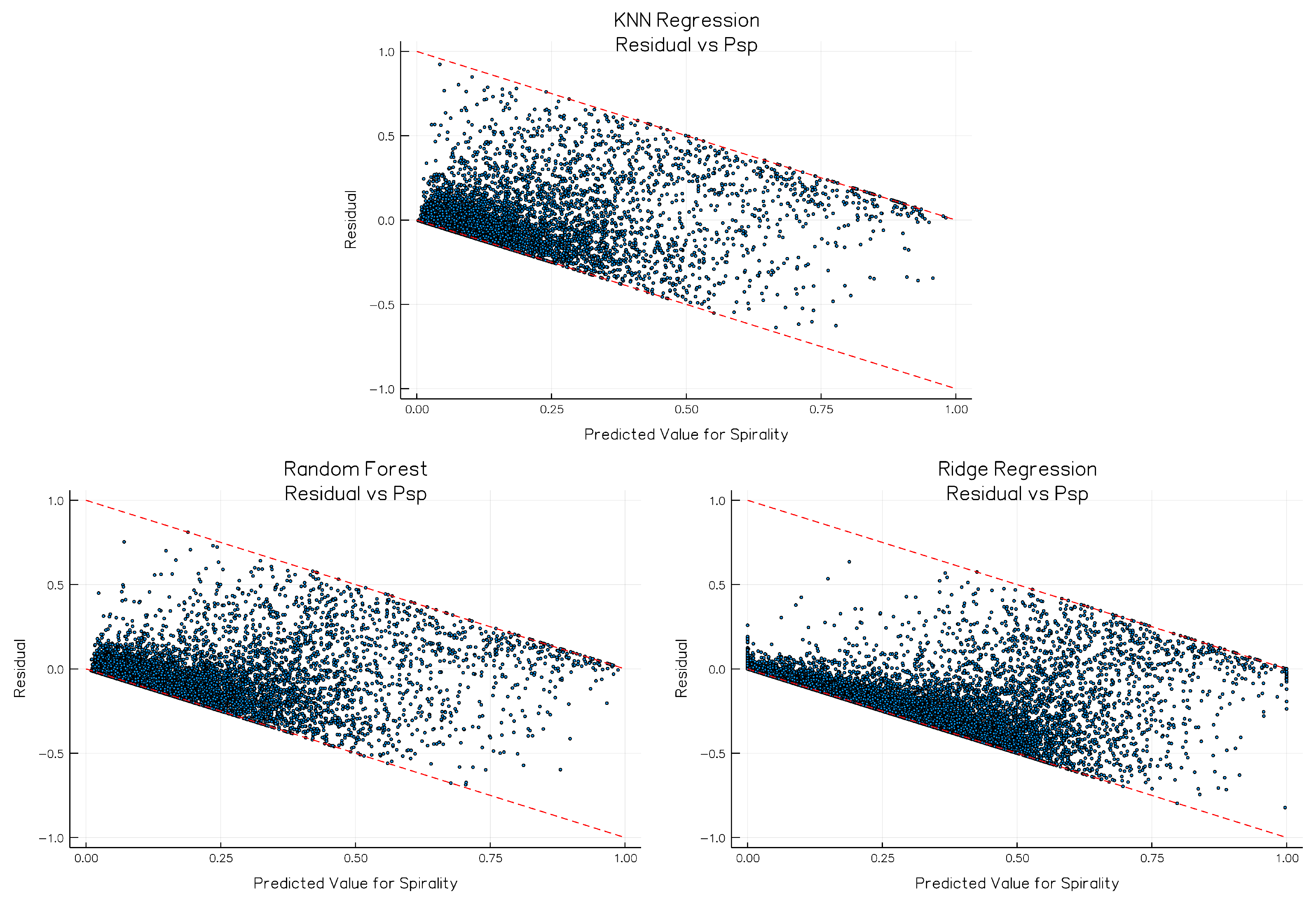
3.4. Comparison with Other Regression Methods
4. Conclusions
Author Contributions
Funding
Acknowledgments
Conflicts of Interest
References
- Smith, R.W. The Expanding Universe: Astronomy’s ‘Great Debate’, 1900–1931; Cambridge University Press: Cambridge, UK, 1982. [Google Scholar]
- Oort, J.H. Problems of Galactic Structure. Astrophys. J. 1952, 116, 233. [Google Scholar] [CrossRef]
- De Vaucouleurs, G. General physical properties of external galaxies. In Astrophysik IV: Sternsysteme/Astrophysics IV: Stellar Systems; Springer: New York, NY, USA, 1959; pp. 311–372. [Google Scholar]
- Perlmutter, S.; Turner, M.S.; White, M. Constraining dark energy with type Ia supernovae and large-scale structure. Phys. Rev. Lett. 1999, 83, 670. [Google Scholar] [CrossRef]
- Nelson, D.; Pillepich, A.; Genel, S.; Vogelsberger, M.; Springel, V.; Torrey, P.; Rodriguez-Gomez, V.; Sijacki, D.; Snyder, G.F.; Griffen, B.; et al. The illustris simulation: Public data release. Astron. Comput. 2015, 13, 12–37. [Google Scholar] [CrossRef]
- Binney, J.; Tremaine, S. Galactic Dynamics; Princeton Series in Astrophysics; Princeton University Press: Princeton, NJ, USA, 1987. [Google Scholar]
- Mihalas, D.; Binney, J. Galactic Astronomy—Structure and Kinematics; Princeton Series in Astrophysics; W.H. Freeman and Co.: San Francisco, CA, USA, 1981. [Google Scholar]
- Lintott, C.J.; Schawinski, K.; Slosar, A.; Land, K.; Bamford, S.P.; Thomas, D.; Raddick, M.J.; Nichol, R.C.; Szalay, A.; Andreescu, D.; et al. Galaxy Zoo: Morphologies derived from visual inspection of galaxies from the Sloan Digital Sky Survey. Mon. Not. R. Astron. Soc. 2008, 389, 1179–1189. [Google Scholar] [CrossRef]
- Davis, D.; Hayes, W. Automated quantitative description of spiral galaxy arm-segment structure. In Proceedings of the 2012 IEEE Conference on Computer Vision and Pattern Recognition, Providence, RI, USA, 16–21 June 2012; pp. 1138–1145. [Google Scholar] [CrossRef]
- Sellwood, J.A. The lifetimes of spiral patterns in disc galaxies. Mon. Not. R. Astron. Soc. 2011, 410, 1637–1646. [Google Scholar] [CrossRef]
- York, D.G.; Adelman, J.; Anderson, J.E., Jr.; Anderson, S.F.; Annis, J.; Bahcall, N.A.; Bakken, J.A.; Barkhouser, R.; Bastian, S.; Berman, E.; et al. The Sloan Digital Sky Survey: Technical summary. Astron. J. 2000, 120, 1579–1587. [Google Scholar] [CrossRef]
- Lintott, C.; Schawinski, K.; Bamford, S.; Slosar, A.; Land, K.; Thomas, D.; Edmondson, E.; Masters, K.; Nichol, R.C.; Raddick, M.J.; et al. Galaxy Zoo 1: Data release of morphological classifications for nearly 900,000 galaxies. Mon. Not. R. Astron. Soc. 2010, 14, 1–14. [Google Scholar] [CrossRef]
- Kahn, S.; Hall, H.J.; Gilmozzi, R.; Marshall, H.K. Final Design of the Large Synoptic Survey Telescope. Proc. SPIE 2016, 9906, 17. [Google Scholar]
- Kalirai, J. Scientific Discovery with the James Webb Space Telescope. arXiv, 2018; arXiv:1805.06941. [Google Scholar]
- Davis, D.R.; Hayes, W.B. SpArcFiRe: Scalable Automated Detection of Spiral Galaxy Arm Segments. Astrophys. J. 2014, 790, 87. [Google Scholar] [CrossRef]
- Davis, D.R. Fast Approximate Quantification of Arbitrary Arm-Segment Structure in Spiral Galaxies. Ph.D. Thesis, University of California, Irvine, CA, USA, 2014. [Google Scholar]
- Lintott, C.J.; Schawinski, K.; Bamford, S.P.; Slosar, A.; Land, K.; Thomas, D.; Edmondson, E.; Masters, K.; Nichol, R.C.; Raddick, M.J.; et al. Galaxy Zoo 1: Data release of morphological classifications for nearly 900,000 galaxies. Neural Netw. 2011, 410, 166–178. [Google Scholar] [CrossRef]
- Land, K.; Slosar, A.; Lintott, C.J.; Andreescu, D.; Bamford, S.P.; Murray, P.; Nichol, R.; Raddick, M.J.; Schawinski, K.; Szalay, A.; et al. Galaxy Zoo: The large-scale spin statistics of spiral galaxies in the Sloan Digital Sky Survey. Mon. Not. R. Astron. Soc. 2008, 388, 1686–1692. [Google Scholar] [CrossRef]
- Hayes, W.B.; Davis, D.R.; Silva, P. On the nature and correction of the spurious S-wise spiral galaxy winding bias in Galaxy Zoo 1. Mon. Not. R. Astron. Soc. 2017, 466, 3928–3936. [Google Scholar] [CrossRef]
- Shamir, L. Automatic morphological classification of galaxy images. Mon. Not. R. Astron. Soc. 2009, 399, 1367–1372. [Google Scholar] [CrossRef] [PubMed]
- Huertas-Company, M.; Aguerri, J.A.L.; Bernardi, M.; Mei, S.; Sánchez Almeida, J. Revisiting the Hubble sequence in the SDSS DR7 spectroscopic sample: A publicly available Bayesian automated classification. Astron. Astrophys. 2010, 525, A157. [Google Scholar] [CrossRef]
- Banerji, M.; Lahav, O.; Lintott, C.J.; Abdalla, F.B.; Schawinski, K.; Bamford, S.P.; Andreescu, D.; Murray, P.; Raddick, M.J.; Slosar, A.; et al. Galaxy Zoo: Reproducing galaxy morphologies via machine learning. Mon. Not. R. Astron. Soc. 2010, 406, 342–353. [Google Scholar] [CrossRef]
- Kuminski, E.; George, J.; Wallin, J.; Shamir, L. Combining Human and Machine Learning for Morphological Analysis of Galaxy Images. Publ. Astrono. Soc. Pac. 2014, 126, 959–967. [Google Scholar] [CrossRef]
- Dieleman, S.; Willett, K.W.; Dambre, J. Rotation-invariant convolutional neural networks for galaxy morphology prediction. Mon. Not. R. Astron. Soc. 2015, 450, 1441–1459. [Google Scholar] [CrossRef]
- Ferrari, F.; de Carvalho, R.R.; Trevisan, M. Morfometryka—A New Way of Establishing Morphological Classification of Galaxies. Astrophys. J. 2015, 814, 55. [Google Scholar] [CrossRef]
- Willett, K.W.; Lintott, C.J.; Bamford, S.P.; Masters, K.L.; Simmons, B.D.; Casteels, K.R.V.; Edmondson, E.M.; Fortson, L.F.; Kaviraj, S.; Keel, W.C.; et al. Galaxy Zoo 2: Detailed morphological classifications for 304 122 galaxies from the Sloan Digital Sky Survey. Mon. Not. R. Astron. Soc. 2013, 435, 2835–2860. [Google Scholar] [CrossRef]
- Abd Elfattah, M.; Elbendary, N.; Elminir, H.K.; Abu El-Soud, M.A.; Hassanien, A.E. Galaxies image classification using empirical mode decomposition and machine learning techniques. In Proceedings of the 2014 International Conference on Engineering and Technology (ICET), Cairo, Egypt, 19–20 April 2014; pp. 1–5. [Google Scholar]
- Applebaum, K.; Zhang, D. Classifying Galaxy Images through Support Vector Machines. In Proceedings of the 2015 IEEE International Conference on Information Reuse and Integration (IRI), San Francisco, CA, USA, 13–15 August 2015; pp. 357–363. [Google Scholar]
- Bishop, C.M. Pattern Recognition and Machine Learning (Information Science and Statistics), 1st ed.; Springer: New York, NY, USA, 2006. [Google Scholar]
- Ribeiro, M.T.; Singh, S.; Guestrin, C. “Why Should I Trust You?”: Explaining the Predictions of Any Classifier. In Proceedings of the 22nd ACM SIGKDD International Conference on Knowledge Discovery and Data Mining (KDD ’16), San Francisco, CA, USA, 19–17 August 2016; ACM: New York, NY, USA, 2016; pp. 1135–1144. [Google Scholar] [CrossRef]
- Nguyen, A.; Yosinski, J.; Clune, J. Deep neural networks are easily fooled: High confidence predictions for unrecognizable images. arXiv, 2015; arXiv:1412.1897. [Google Scholar]
- Peng, T.; English, J.E.; Silva, P.; Davis, D.R.; Hayes, W.B. SpArcFiRe: Morphological selection effects due to reduced visibility of tightly winding arms in distant spiral galaxies. arXiv, 2017; arXiv:1707.02021. [Google Scholar] [CrossRef]
- Hall, M.; Frank, E.; Holmes, G.; Pfahringer, B.; Reutemann, P.; Witten, I.H. The WEKA data mining software: An update. ACM SIGKDD Explor. Newsl. 2009, 11, 10–18. [Google Scholar] [CrossRef]
- Adelman-McCarthy, J.K.; Agüeros, M.A.; Allam, S.S.; Prieto, C.A.; Anderson, K.S.J.; Anderson, S.F.; Annis, J.; Bahcall, N.A.; Bailer-Jones, C.A.L.; Baldry, I.K.; et al. The Sixth Data Release of the Sloan Digital Sky Survey. Astrophys. J. Suppl. Ser. 2008, 175, 297–313. [Google Scholar] [CrossRef]
- Bezanson, J.; Edelman, A.; Karpinski, S.; Shah, V.B. Julia: A Fresh Approach to Numerical Computing. Soc. Ind. Appl. Math. Rev. 2017, 59, 65–98. [Google Scholar] [CrossRef]
- Sibley, C. More Is Always Better: The Power Of Simple Ensembles. 2012. Available online: http://www.overkillanalytics.net/more-is-always-better-the-power-of-simple-ensembles/ (accessed on 1 September 2018).
- Refaeilzadeh, P.; Tang, L.; Liu, H. Cross-Validation. In Encyclopedia of Database Systems; Springer: New York, NY, USA, 2016; pp. 1–7. [Google Scholar]
- James, G.; Witten, D.; Hastie, T.; Tibshirani, R. An Introduction to Statistical Learning: With Applications in R; Springer: New York, NY, USA, 2014; p. 70. [Google Scholar]
- Kuhn, M.; Johnson, K. Applied Predictive Modeling; Springer: New York, NY, USA, 2013; p. 184. [Google Scholar]
- Rahman, N. A Course in Theoretical Statistics: For Sixth forms, Technical Colleges, Colleges of Education, Universities; Charles Griffin & Company Limited: London, UK, 1968. [Google Scholar]
- Jensen, R.; Shen, Q. Are More Features Better? A Response to Attributes Reduction Using Fuzzy Rough Sets. IEEE Trans. Fuzzy Syst. 2009, 17, 1456–1458. [Google Scholar] [CrossRef]
- Saabas, A. Selecting Good Features Part III: Random Forests. 2014. Available online: https://blog.datadive.net/selecting-good-features-part-iii-random-forests/ (accessed on 1 September 2018).
| 1 | Stephen Bamford, Personal Communication. |
| 2 | In essence, comparing against the Gold sample says “look how well we do when the humans pre-select the easy ones for us!” More formally, it disregards false positives—galaxies which the prediction is confident but is actually way off. |
| 3 | It is important to clarify that throughout this paper we will be using the term feature(s) to describe an individual measurable property or characteristic of a phenomenon being observed [29] as it is commonly done in the machine learning literature as opposed to features as seen in an image-like globular clusters. |
| 4 | High spirality is a strong indicator of a galaxy being spiral, but it’s not a necessary condition. Galaxies with low spirality may be edge-on spirals, ellipticals, low-resolution spirals, or even disk galaxies without spiral structure, such as the Sombrero Galaxy. |
| 5 | K-Fold cross validation is a method for measuring the quality of a learning algorithm by splitting the data into K buckets, training the algorithm in of these buckets and testing in the holdout bucket. We do this K times, each time holding out a different bucket and we report the average accuracy as the final accuracy of a model in that dataset. Finally, we choose the best out of the K models as our final model, having demonstrated that all the other K-1 models also perform reasonably well. |
| 6 | A higher accuracy can be achieved if we use a boundary below 0.5. Note that, since there were six choices in GZ1, any vote receiving more than 1/6 of the votes can be a winning vote; for example, a vote of 40% could be considered a classification if all the other choices had less than 40% of votes. It is also possible to get better accuracy, using the same features, if we build a classifier rather than a regressor, but that is outside the scope of this paper. |
| 7 | One might argue that perhaps our “spirality” measure is more aptly called “non-ellipticity”. |


| Name | Description |
|---|---|
| C&P set | colors and profile fitting |
| color, deredenned | |
| color, deredenned | |
| de Vaucouleurs fit axial ratio | |
| exponential fit axial ratio | |
| exponential disk fit log likelihood | |
| de Vaucouleurs fit log likelihood | |
| Star log likelihood | |
| Absolute magnitudes in the 5 color bands | |
| AM set | adaptive moments |
| concentration | |
| adaptive (+) shape measure | |
| adaptive ellipticity | |
| adaptive 4th moment | |
| texture parameter |
| pair | p1 | p2 | p3 | p4 | correctAll | SPcapture | SPcontam |
|---|---|---|---|---|---|---|---|
| 0.20 | 0.30 | 0.52 | 0.51 | 65.7% | 42.0% | 48.7% | |
| 0.12 | 0.65 | 0.38 | 0.85 | 74.3% | 32.4% | 14.8% |
| Feature | Description |
|---|---|
| bar_scores | SpArcFiRe’s various bar detection scores |
| avg(abs(pa))-abs(avg(pa)) | pitch angle-weighted chirality consistency across arms |
| numArcs > L | SpArcFiRe’s count of arms of various lengths |
| numDcoArcs > L | SpArcFiRe’s count of dominant-chirality-only arms of various lengths (see text) |
| totalNumArcs | total number of arcs found by SpArcFiRe |
| totalArcLen | total length of all arcs found by SpArcFiRe |
| avgArcLen | average arc length across arcs found by SpArcFiRe |
| arcLenAtXX% | length of arc at XX = 25%, 50%, and 75% of total length of arcs (see text) |
| rankAtXX% | arc rank at XX = 25%, 50%, and 75% of total length of arcs (see text) |
| bulgeAxisRatio | axis ratio of bulge, if present |
| diskAxisRatio | axis ratio of entire galaxy image; values suggest an edge-on spiral rather than elliptical |
| disk/bulgeRatio | disk to bulge ratio |
| diskBulgeAxisRatio | ratio of (diskAxisRatio) / (bulgeAxisRatio) |
| gaussLogLik | Gauss Log Likelihood of ellipse fit |
| likelihoodCtr | likelihood of the center of the ellipse fit |
| abs(pa_alen_avg) | average pitch angle of arms, length-weighted |
| abs(pa_alen_avg_DCO) | average pitch angle only of arms of dominant chirality |
| twoLongestAgree | chirality agreement of two longest arcs (Boolean) |
| Total #Features | Features/Tree | # of Trees | Feature(s) | Correct |
|---|---|---|---|---|
| 1 | 1 | 1 | Color only | 65% |
| 1 | 1 | 1 | Magnitude only | 65% |
| 2 | 2 | 1 | color + mag | 75% |
| 3 | 3 | 1 | col,mag,arcs | 85% |
| 7 | 7 | 1 | various | ∼90% |
| 35 | 7 | 10 | various | ∼95% |
| 35 | 7 | 50 | various | ∼97% |
| 101 | 7 | 100 | various | 99.9% |
| \ | 0.0–0.1 | 0.1–0.2 | 0.2–0.3 | 0.3–0.4 | 0.4–0.5 | 0.5–0.6 | 0.6–0.7 | 0.7–0.8 | 0.8–0.9 | 0.9–1.0 | TOTAL |
|---|---|---|---|---|---|---|---|---|---|---|---|
| 0.0–0.1 | 21,238 | 5042 | 1512 | 522 | 169 | 45 | 17 | 1 | 1 | 1 | 28,548 |
| 0.1–0.2 | 2471 | 1803 | 1145 | 594 | 254 | 111 | 28 | 5 | 0 | 0 | 6411 |
| 0.2–0.3 | 509 | 761 | 668 | 522 | 233 | 96 | 42 | 14 | 7 | 0 | 2852 |
| 0.3–0.4 | 184 | 345 | 424 | 348 | 209 | 120 | 58 | 23 | 5 | 2 | 1718 |
| 0.4–0.5 | 62 | 187 | 243 | 268 | 191 | 93 | 56 | 33 | 8 | 1 | 1142 |
| 0.5–0.6 | 47 | 128 | 215 | 200 | 188 | 145 | 76 | 38 | 11 | 3 | 1051 |
| 0.6–0.7 | 30 | 99 | 149 | 175 | 138 | 113 | 76 | 53 | 19 | 6 | 858 |
| 0.7–0.8 | 23 | 70 | 91 | 123 | 120 | 121 | 108 | 80 | 42 | 7 | 785 |
| 0.8–0.9 | 21 | 38 | 89 | 107 | 144 | 136 | 148 | 134 | 80 | 24 | 921 |
| 0.9–1.0 | 4 | 32 | 53 | 87 | 129 | 151 | 211 | 257 | 289 | 303 | 1516 |
| TOTAL | 24,589 | 8505 | 4589 | 2946 | 1775 | 1131 | 820 | 638 | 462 | 347 | 45,802 |
| Feature | Score | Standard Deviation |
|---|---|---|
| Number of dominant-chirality-only arms equal or longer than 120 | 0.039 | 0.080 |
| Absolute Magnitude in the Z band | 0.031 | 0.020 |
| De-reddened magnitude in the R band | 0.029 | 0.019 |
| De Vaucoleurs fit axial ratio i band | 0.028 | 0.013 |
| Number of dominant-chirality-only arms equal or longer than 85 | 0.022 | 0.061 |
| Number of dominant-chirality-only arms equal or longer than 100 | 0.022 | 0.057 |
| Number of arcs equal or longer than 120 | 0.022 | 0.057 |
| Exponential fit axial ratio i band | 0.021 | 0.009 |
| De-reddened magnitude in the G band | 0.021 | 0.015 |
| Number of dominant-chirality-only arms equal or longer than 80 | 0.021 | 0.060 |
| Measure\Model | Random Forest | Ridge Regression | K-Nearest Neighbors |
|---|---|---|---|
| Pearson Correlation (PC) | 0.8631 | 0.6753 | 0.7729 |
| Root Mean Squared Error (RMSE) | 0.1381 | 0.2495 | 0.1426 |
| Mean Absolute Error (MAE) | 0.0713 | 0.2011 | 0.0872 |
| Mean Error (ME) | −0.00007 | 0.1789 | −0.0025 |
© 2018 by the authors. Licensee MDPI, Basel, Switzerland. This article is an open access article distributed under the terms and conditions of the Creative Commons Attribution (CC BY) license (http://creativecommons.org/licenses/by/4.0/).
Share and Cite
Silva, P.; Cao, L.T.; Hayes, W.B. SpArcFiRe: Enhancing Spiral Galaxy Recognition Using Arm Analysis and Random Forests. Galaxies 2018, 6, 95. https://doi.org/10.3390/galaxies6030095
Silva P, Cao LT, Hayes WB. SpArcFiRe: Enhancing Spiral Galaxy Recognition Using Arm Analysis and Random Forests. Galaxies. 2018; 6(3):95. https://doi.org/10.3390/galaxies6030095
Chicago/Turabian StyleSilva, Pedro, Leon T. Cao, and Wayne B. Hayes. 2018. "SpArcFiRe: Enhancing Spiral Galaxy Recognition Using Arm Analysis and Random Forests" Galaxies 6, no. 3: 95. https://doi.org/10.3390/galaxies6030095
APA StyleSilva, P., Cao, L. T., & Hayes, W. B. (2018). SpArcFiRe: Enhancing Spiral Galaxy Recognition Using Arm Analysis and Random Forests. Galaxies, 6(3), 95. https://doi.org/10.3390/galaxies6030095