A Left and Right Truncated Schechter Luminosity Function for Quasars

Abstract

The luminosity function for quasars (QSOs) is usually fitted by a Schechter function. The dependence of the number of quasars on the redshift, both in the low and high luminosity regions, requires the inclusion of a lower and upper boundary in the Schechter function. The normalization of the truncated Schechter function is forced to be the same as that for the Schechter function, and an analytical form for the average value is derived. Three astrophysical applications for QSOs are provided: deduction of the parameters at low redshifts, behavior of the average absolute magnitude at high redshifts, and the location (in redshift) of the photometric maximum as a function of the selected apparent magnitude. The truncated Schechter function with the double power law and an improved Schechter function are compared as luminosity functions for QSOs. The chosen cosmological framework is that of the flat cosmology, for which we provided the luminosity distance, the inverse relation for the luminosity distance, and the distance modulus.

1. Introduction

The Schechter function was first introduced in order to model the luminosity function (LF) for galaxies (see [1]), and later was used to model the LF for quasars (QSOs) (see [2,3]). Over the years, other LFs for galaxies have been suggested, such as a two-component Schechter-like LF (see [4]), the hybrid Schechter+power-law LF to fit the faint end of the K-band (see [5]), and the double Schechter LF, see Blanton et al. [6]. In order to improve the flexibility at the bright end, a new parameter $\eta$ was introduced in the Schechter LF, see [7]. The above discussion suggests the introduction of finite boundaries for the Schechter LF rather than the usual zero and infinity. As a practical example, the most luminous QSOs have absolute magnitude $M_{b_j}\approx -28$ or the luminosity is not ∞ and the less luminous QSOs have have absolute magnitude $M_{b_j}\approx -20$ or the luminosity is not zero (see Figure 19 in [8]). A physical source of truncation at the low luminosity boundary (high absolute magnitude) is the fact that with increasing redshift the less luminous QSOs progressively disappear. In other words, the upper boundary in absolute magnitude for QSOs is a function of the redshift.

The suggestion to introduce two boundaries in a probability density function (PDF) is not new and, as an example, Ref. [9] considered a doubly-truncated gamma PDF restricted by both a lower (l) and upper (u) truncation. A way to deduce a new truncated LF for galaxies or QSOs is to start from a truncated PDF and then derive the magnitude version. This approach has been used to deduce a left truncated beta LF (see [10,11]), and a truncated gamma LF (see [12]).

The main difference between LFs for galaxies and for QSOs is that, in the first case, we have an LF for a unit volume of 1 ${\mathrm{Mpc}}^3$ and, in the second case, we are speaking of an LF for unit volume but with a redshift dependence. The dependence on the redshift complicates an analytical approach because the number of observed QSOs at low luminosity decreases with the redshift, and the highest observed luminosity increases with the redshift. The first effect is connected with the Malmquist bias, i.e., the average luminosity increases with the redshift, and the second one can be modeled by an empirical law. The above redshift dependence in the case of QSOs can be modeled by the double power law LF (see [13]), or by an improved Schechter function (see [14]). The present paper derives, in Section 2, the luminosity distance and the distance modulus in a flat cosmology. Section 3 derives a truncated version of the Schechter LF. Section 4 applies the truncated Schechter LF to QSOs, deriving the parameters of the LF in the range of redshift $[0.3,0.5]$, modeling the average absolute magnitude as a function of the redshift, and deriving the photometric maximum for a given apparent magnitude as a function of the redshift.

2. The Flat Cosmology

The first definition of the luminosity distance, $d_{\mathrm{L}}$, in flat cosmology is

$$d_{\mathrm{L}}(z;c,H_0,{\Omega }_{\mathrm{M}})=\frac{c}{H_0}(1+z){\int }_{\frac{1}{1+z}}^1\frac{da}{\sqrt{{\Omega }_{\mathrm{M}}a+(1-{\Omega }_{\mathrm{M}})a^4}},$$

(1)

where $H_0$ is the Hubble constant expressed in $\mathrm{km}{\mathrm{s}}^{-1}{\mathrm{Mpc}}^{-1}$, c is the speed of light expressed in $\mathrm{km}{\mathrm{s}}^{-1}$, z is the redshift, a is the scale-factor, and ${\Omega }_{\mathrm{M}}$ is

$${\Omega }_{\mathrm{M}}=\frac{8\pi G{\rho }_0}{3H_0^2},$$

(2)

where G is the Newtonian gravitational constant and ${\rho }_0$ is the mass density at the present time, see Equation (2.1) in [15]. A second definition of the luminosity distance is

$$d_{\mathrm{L}}(z;c,H_0,{\Omega }_{\mathrm{M}})=\frac{c}{H_0}(1+z){\int }_0^z\frac{1}{\sqrt{{\left(1+z\right)}^3{\Omega }_{\mathrm{M}}+1-{\Omega }_{\mathrm{M}}}}\mathrm{d}z,$$

(3)

see Equation (2) in [16]. The change of variable $z=-1+1/a$ in the second definition allows finding the first definition. An analytical expression for the integral (1) is here reported as a Taylor series of order 8 when ${\Omega }_{\mathrm{M}}=0.3$ and $H_0=70$ $\mathrm{km}{\mathrm{s}}^{-1}{\mathrm{Mpc}}^{-1}$

$$\begin{array}{cc}\hfill d_{\mathrm{L}}\left(z\right)=& 4282.74(1+z)(2.45214+0.01506{(1+z)}^{-8}-0.06633{(1+z)}^{-7}\hfill \\ & -0.01619{(1+z)}^{-6}+0.60913{(1+z)}^{-5}-1.29912{(1+z)}^{-4}+0.406124{(1+z)}^{-3}\hfill \\ & +2.47428{(1+z)}^{-2}-4.57509{(1+z)}^{-1})\mathrm{Mpc},\hfill \end{array}$$

(4)

and the distance modulus as a function of z, $F\left(z\right)$,

$$\begin{array}{c}\hfill (m-M)=F\left(z\right)=43.15861+2.17147ln(7.77498z^2+2.45214z^8+15.0420z^7+39.1085z^6\\ \hfill +56.4947z^5+49.3673z^4+26.1512z^3+0.99999z+1.73{10}^{-7})-15.2003ln(1+z).\end{array}$$

(5)

As a consequence, the absolute magnitude, M, is

$$M=m-F\left(z\right).$$

(6)

The angular diameter distance, $D_A$, after [17], is

$$D_A=\frac{D_L}{{(1+z)}^2}.$$

(7)

We may approximate the luminosity distance as given by Equation (4) by the minimax rational approximation, $d_{L,2,1}$, with the degree of the numerator $p=2$ and the degree of the denominator $q=1$:

$$d_{L,2,1}\left(z\right)=\frac{4.10871+1813.96z+2957.04z^2}{0.44404+0.27797z},$$

(8)

which allows deriving the inverse formula, the redshift, as a function of the luminosity distance:

$$\begin{array}{cc}\hfill z_{2,1}\left(d_{\mathrm{L}}\right)=& 0.000047d_{\mathrm{L}}-0.306718\hfill \\ & +3.38175\times {10}^{-14}\sqrt{1.9318{10}^{18}{d_{\mathrm{L}}}^2+1.06093\times {10}^{23}{d}_{\mathrm{L}}+8.10464\times {10}^{25}}.\hfill \end{array}$$

(9)

Another useful distance is the transverse comoving distance, $D_M$,

$$D_M=\frac{D_L}{1+z},$$

(10)

with the connected total comoving volume $V_c$

$$V_c=\frac{4}{3}\pi D_M^3,$$

(11)

which can be minimax-approximated as

$$V_{c,3,2}=\frac{3.01484{10}^{10}{z}^3+6.39699{10}^{10}{z}^2-1.26793{10}^{10}z+4.10104{10}^8}{0.45999-0.01011z+0.093371z^2}Mp{c}^3.$$

(12)

3. The Adopted LFs

This section reviews the Schechter LF, the double power law LF, and the Pei LF for QSOs. The truncated version of the Schechter LF is derived. The merit function ${\chi }^2$ is computed as

$${\chi }^2=\sum _{j=1}^n{(\frac{L{F}_{theo}-L{F}_{astr}}{{\sigma }_{L{F}_{astr}}})}^2,$$

(13)

where n is the number of bins for LF of QSOs and the two indices $theo$ and $astr$ stand for ‘theoretical’ and ‘astronomical’, respectively. The residual sum of squares (RSS) is

$$RSS=\sum _{j=1}^n{(y{\left(i\right)}_{theo}-y{\left(i\right)}_{astr})}^2,$$

(14)

where $y{\left(i\right)}_{theo}$ is the theoretical value and $y{\left(i\right)}_{astr}$ is the astronomical value.

A reduced merit function ${\chi }_{red}^2$ is evaluated by

$${\chi }_{red}^2={\chi }^2/NF,$$

(15)

where $NF=n-k$ is the number of degrees of freedom and k is the number of parameters. The goodness of the fit can be expressed by the probability Q (see Equation 15.2.12 in [18], which involves the degrees of freedom and the ${\chi }^2$). According to [18], the fit “may be acceptable” if $Q>0.001$. The Akaike information criterion (AIC) (see [19]), is defined by

$$AIC=2k-2ln\left(L\right),$$

(16)

where L is the likelihood function and k is the number of free parameters in the model. We assume a Gaussian distribution for the errors and the likelihood function can be derived from the ${\chi }^2$ statistic $L\propto exp(-\frac{{\chi }^2}{2}),$ where ${\chi }^2$ has been computed by Equation (13), see [20,21]. Now, the AIC becomes

$$AIC=2k+{\chi }^2.$$

(17)

3.1. The Schechter LF

Let L be a random variable taking values in the closed interval $[0,\infty ]$. The Schechter LF of galaxies, after [1], is

$$\mathrm{\Phi }(L;{\mathrm{\Phi }}^{*},\alpha ,L^{*})dL=(\frac{{\mathrm{\Phi }}^{*}}{L^{*}}){(\frac{L}{L^{*}})}^{\alpha }exp(-\frac{L}{L^{*}})dL,$$

(18)

where $\alpha$ sets the slope for low values of L, $L^{*}$ is the characteristic luminosity, and ${\mathrm{\Phi }}^{*}$ represents the number of galaxies per $Mp{c}^3$. The normalization is

$${\int }_0^{\infty }\mathrm{\Phi }(L;{\mathrm{\Phi }}^{*},\alpha ,L^{*})dL={\mathrm{\Phi }}^{*}\mathrm{\Gamma }\left(\alpha +1\right),$$

(19)

where

$$\mathrm{\Gamma }\left(z\right)={\int }_0^{\infty }{e}^{-t}{t}^{z-1}dt,$$

(20)

is the gamma function. The average luminosity, $⟨L⟩$, is

$$⟨L({\mathrm{\Phi }}^{*},\alpha ,L^{*})⟩=L^{*}{\mathrm{\Phi }}^{*}\mathrm{\Gamma }\left(\alpha +2\right).$$

(21)

An equivalent form in absolute magnitude of the Schechter LF is

$$\mathrm{\Phi }(M;{\mathrm{\Phi }}^{*},\alpha ,M^{*})dM=0.921{\mathrm{\Phi }}^{*}{10}^{0.4(\alpha +1)(M^{*}-M)}exp(-{10}^{0.4(M^{*}-M)})dM,$$

(22)

where $M^{*}$ is the characteristic magnitude. The scaling with h is $M^{*}-5{log}_{10}h$ and ${\mathrm{\Phi }}^{*}{h}^3$ [${\mathrm{Mpc}}^{-3}$].

3.2. The Truncated Schechter LF

We assume that the luminosity L takes values in the interval $[L_l,L_u]$, where the indices l and u mean ‘lower’ and ‘upper’; the truncated Schechter LF, $S_T$, is

$$S_T(L;{\mathrm{\Psi }}^{*},\alpha ,L^{*},L_l,L_u)=\frac{-{\left(\frac{L}{{\mathit{L}}^{*}}\right)}^{\alpha }{\mathrm{e}}^{-\frac{L}{L^{*}}}{\Psi }^{*}\mathrm{\Gamma }\left(\alpha +1\right)}{{\mathit{L}}^{*}\left(\mathrm{\Gamma }\left(\alpha +1,\frac{L_u}{L^{*}}\right)-\mathrm{\Gamma }\left(\alpha +1,\frac{L_l}{L^{*}}\right)\right)},$$

(23)

where $\mathrm{\Gamma }(a,z)$ is the incomplete Gamma function defined as

$$\mathrm{\Gamma }\left(a,z\right)={\int }_z^{\infty }{t}^{a-1}{e}^{-t}dt,$$

(24)

see [22]. The normalization is the same as for the Schechter LF, see Equation (19),

$${\int }_0^{\infty }{S}_T(L;{\mathrm{\Psi }}^{*},\alpha ,L^{*},L_l,L_u)dL={\mathrm{\Psi }}^{*}\mathrm{\Gamma }\left(\alpha +1\right).$$

(25)

The average value is

$$⟨L({\mathrm{\Psi }}^{*},\alpha ,L^{*},L_l,L_u)⟩=\frac{N}{L^{*}\left(\mathrm{\Gamma }\left(\alpha +1,\frac{L_u}{L^{*}}\right)-\mathrm{\Gamma }\left(\alpha +1,\frac{L_l}{L^{*}}\right)\right)}$$

(26)

with

$$\begin{array}{cc}\hfill N=& {\Psi }^{*}(L^{*2}\mathrm{\Gamma }(\alpha +1,\frac{L_u}{L^{*}})\alpha -{L^{*}}^2\mathrm{\Gamma }(\alpha +1,\frac{L_l}{L^{*}})\alpha +{L^{*}}^2\mathrm{\Gamma }(\alpha +1,\frac{L_u}{L^{*}})\hfill \\ & -{L^{*}}^2\mathrm{\Gamma }(\alpha +1,\frac{L_l}{L^{*}})-{L^{*}}^{-\alpha +1}{\mathrm{e}}^{-\frac{L_l}{L^{*}}}{L_l}^{\alpha +1}+{L^{*}}^{-\alpha +1}{\mathrm{e}}^{-\frac{L_u}{L^{*}}}{L_u}^{\alpha +1})\mathrm{\Gamma }\left(\alpha +1\right).\hfill \end{array}$$

(27)

The four luminosities $L,L_l,L^{*}$ and $L_u$ are connected with the absolute magnitudes M, $M_l$, $M_u$ and $M^{*}$ through the following relationship:

$$\frac{L}{L_{\odot }}={10}^{0.4(M_{\odot }-M)},\frac{L_l}{L_{\odot }}={10}^{0.4(M_{\odot }-M_u)},\frac{L^{*}}{L_{\odot }}={10}^{0.4(M_{\odot }-M^{*})},\frac{L_u}{L_{\odot }}={10}^{0.4(M_{\odot }-M_l)},$$

(28)

where the indices u and l are inverted in the transformation from luminosity to absolute magnitude and $L_{\odot }$ and $M_{\odot }$ are the luminosity and absolute magnitude of the sun in the considered band. The equivalent form in absolute magnitude of the truncated Schechter LF is therefore

$$\begin{array}{c}\hfill \mathrm{\Psi }(M;{\mathrm{\Psi }}^{*},\alpha ,M^{*},M_l,M_u)dM=\\ \hfill \frac{-0.4{\left({10}^{0.4M^{*}-0.4M}\right)}^{\alpha }{\mathrm{e}}^{-{10}^{0.4M^{*}-0.4M}}{\mathrm{\Psi }}^{*}\mathrm{\Gamma }\left(\alpha +1\right){10}^{0.4M^{*}-0.4M}\left(ln\left(2\right)+ln\left(5\right)\right)}{\mathrm{\Gamma }\left(\alpha +1,{10}^{-0.4M_l+0.4M^{*}}\right)-\mathrm{\Gamma }\left(\alpha +1,{10}^{0.4M^{*}-0.4M_u}\right)}.\end{array}$$

(29)

The averaged absolute magnitude is

$$⟨M({\mathrm{\Psi }}^{*},\alpha ,L^{*},L_l,L_u)⟩=\frac{{\int }_{M_l}^{M_u}M(M;{\mathrm{\Psi }}^{*},\alpha ,L^{*},L_l,L_u)MdM}{{\int }_{M_l}^{M_u}M(M;{\mathrm{\Psi }}^{*},\alpha ,L^{*},L_l,L_u)dM}.$$

(30)

3.3. The Double Power Law

The double power law LF for QSOs is

$$\mathrm{\Phi }(L;{\varphi }^{*},\alpha ,\beta ,L^{*})=\frac{{\varphi }^{*}}{{(L/L^{*})}^{\alpha }+{(L/L^{*})}^{\beta }},$$

(31)

where $L^{*}$ is the characteristic luminosity, $\alpha$ models the low boundary, and $\beta$ models the high boundary, see [8,13,23,24,25,26]. The magnitude version is

$$\mathrm{\Phi }(M;{\varphi }^{*},\alpha ,\beta ,M^{*})=\frac{{\varphi }^{*}}{{10}^{0.4(\alpha +1)[M-M^{*}]}+{10}^{0.4(\beta +1)[M-M^{*}]}},$$

(32)

where the characteristic absolute magnitude, $M^{*}$, and ${\varphi }^{*}$ are functions of the redshift.

3.4. The Pei Function

The exponential $L^{1/4}$ LF, or Pei LF, after [14], is

$$\mathrm{\Phi }(L;{\varphi }^{*},\beta ,L^{*})=\frac{C{E}^{*}{\left(\frac{L}{L^{*}}\right)}^{-\beta }{\mathrm{e}}^{-\sqrt[4]{\frac{L}{L^{*}}}}}{L^{*}},$$

(33)

and the magnitude version is

$$\mathrm{\Phi }(M;{\varphi }^{*},\beta ,M^{*})=\frac{0.4C{E}^{*}{\left(\frac{{10}^{-0.4M}}{{10}^{-0.4M^{*}}}\right)}^{-\beta }{\mathrm{e}}^{-\sqrt[4]{\frac{{10}^{-0.4M}}{{10}^{-0.4M^{*}}}}}{10}^{-0.4M}ln\left(10\right)}{{10}^{-0.4M^{*}}}.$$

(34)

4. The Astrophysical Applications

This section explains the K-correction for QSOs, introduces the sample of QSOs on which the various tests are performed, finds the parameters of the new LF in the range of redshift $[0.3,0.5]$, and finds the number of QSOs as a function of the redshift.

4.1. K-Correction

The K-correction for QSOs as a function of the redshift can be parametrized as

$$K\left(z\right)=-2.5(1+{\alpha }_{\nu })log(1+z),$$

(35)

with $-0.7<{\alpha }_{\nu }<-0.3$ (see [27]). Following [28], we have adopted ${\alpha }_{\nu }=-0.3$. The corrected absolute magnitude, $M_K$, is

$$M_K=M+K\left(z\right).$$

(36)

In the following, both the observed and the theoretical absolute magnitude will always be K-corrected.

4.2. The Sample of QSO

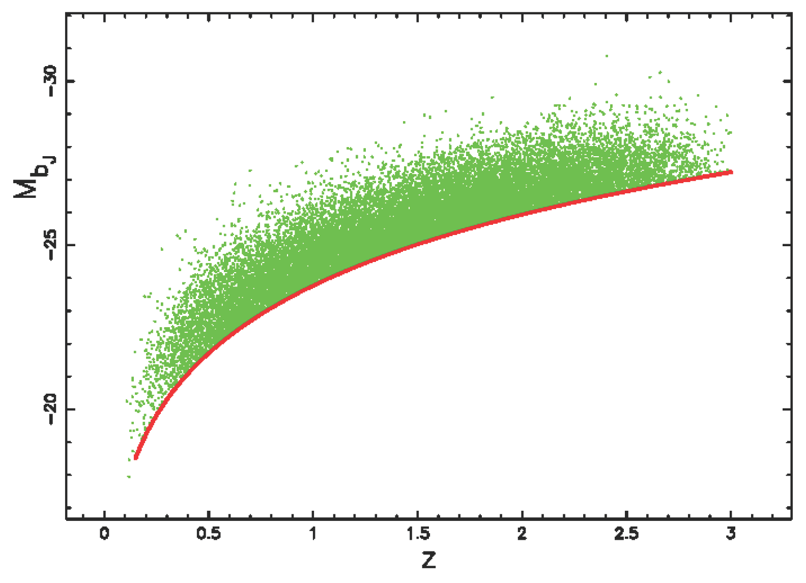
We selected the catalog of the 2dF QSO Redshift Survey (2QZ), which contains 22,431 redshifts of QSOs with $18.25<b_J<20.85$, a total survey area of 721.6 ${deg}^2$, and an effective area of 673.4 ${deg}^2$, see [8] 1. Section 3 in [8] discusses four separate types of completeness that characterize the 2QZ and 6QZ surveys: (i) morphological completeness, $f_m(bJ,z)$, (ii) photometric completeness, $f_p(bJ,z)$, (iii) coverage completeness $f_c\left(\theta \right)$ and (iv) spectroscopic completeness, $f_s(bJ,z,\theta )$. The first test can be done on the upper limit of the maximum absolute magnitude, $M_u\left(z\right)$, which can be observed in a catalog of QSOs characterized by a given limiting magnitude, in our case $b_j=20.85$, where $F\left(z\right)$ has been defined by Equation (5):

$$M_u\left(z\right)=20.85-F\left(z\right)$$

(37)

(see Figure 1).

Figure 1. The absolute magnitude $M_{B_{bj}}$ computed with the nonlinear Equation (36) for 22,413 QSOs versus the redshift (green points). The lower theoretical curve (upper absolute magnitude) as represented by the nonlinear Equation (37) is the red thick line. The redshifts cover the range $[0,3]$.

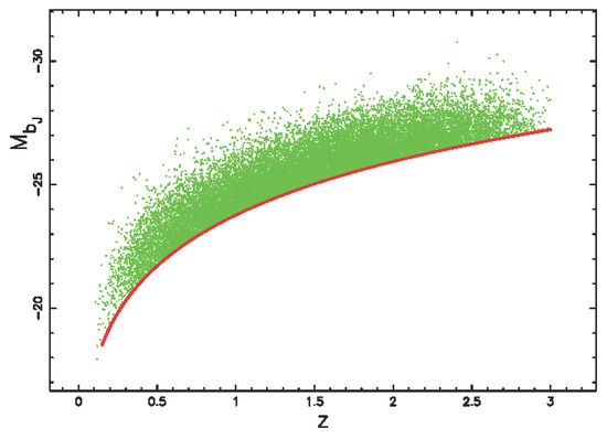
A careful examination of Figure 1 allows concluding that all of the QSOs are in the region over the border line, the number of observed QSOs decreases with increasing z, and the average absolute magnitude decreases with increasing z. The previous comments can be connected with the Malmquist bias, see [29,30], which was originally applied to the stars and later on to the galaxies by [31].

4.3. The Luminosity Function for QSOs

A binned luminosity function for quasars can be built in one of the two methods suggested by [32]: the $\frac{1}{V_a}$ method (see [33,34,35]), and a binned approximation. Notably, Ref. [36] argued that both the $\frac{1}{V_a}$ and the binned approximation can produce bias at the faint end of the LF due to the arbitrary choosing of redshift and luminosity intervals.

We implemented the binned approximation of [32], ${\varphi }_{est}$, as

$$\varphi \approx {\varphi }_{est}=\frac{N_q}{{\int }_{M_{min}}^{M_{max}}{\int }_{z_{min}}^{z_{max}\left(M\right)}\frac{dV}{dz}dzdM},$$

(38)

where $N_q$ is the number of quasars observed in the $M_i-z$ bin. The error is evaluated as

$$\delta {\varphi }_{est}=\frac{\sqrt{N_q}}{{\int }_{M_{min}}^{M_{max}}{\int }_{z_{min}}^{z_{max}\left(M\right)}\frac{dV}{dz}dzdM}.$$

(39)

The comoving volume in the flat cosmology is evaluated according to Equation (11),

$$V=\frac{4}{3}\pi (D_{M,upp}^3-D_{M,low}^3),$$

(40)

where $D_{M,upp}$ and $D_{M,low}$ are, respectively, the upper and lower comoving distance. A correction for the effective volume of the catalog, $V_q$, gives

$$V_q=V\frac{A_{e}de{g}^2}{41252.9de{g}^2},$$

(41)

where $A_e$ is the effective area of the catalog in $de{g}^2$.

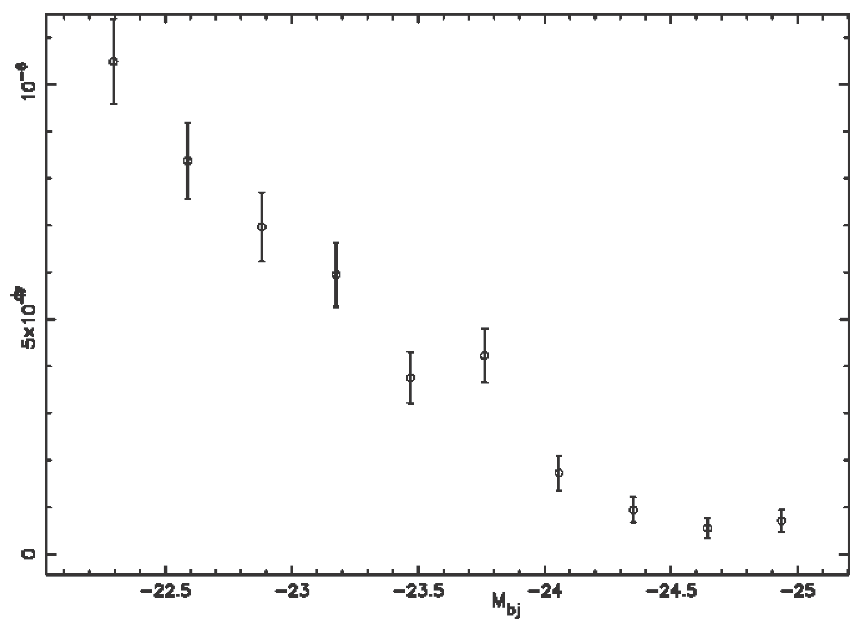
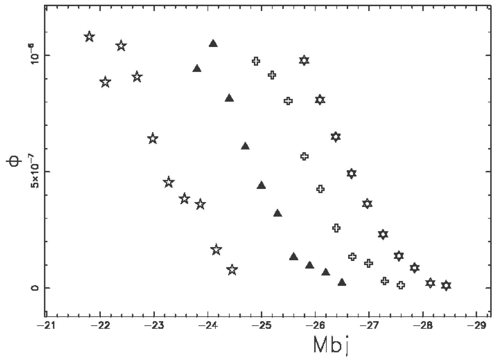
A typical example of the observed LF for QSOs when $0.3<z<0.5$ is reported in Figure 2 and Figure 3 reports the LF for QSOs in four ranges of redshifts.

Figure 2. The observed LF for QSOs is reported with the error bar evaluated as the square root of the LF (Poissonian distribution) when z$[0.3,0.5]$.

Figure 3. The observed LF for QSOs when z $[0.3,0.5]$ and M $[-24.45,-21.50]$ (empty stars), $[0.7,0.9]$ and M $[-26.49,-23.50]$ (full triangles), $[1.1,1.3]$ and M $[-27.59,-24.60]$ (empty crosses) and $[1.5,1.7]$ and M $[-28.43,-25.50]$ (stars of David).

The variable lower bound in absolute magnitude, $M_l$, can be connected with evolutionary effects, and the upper bound, $M_u$, is fixed by the physics (see the nonlinear Equation (37) and see Section 4.4).

The five parameters of the the best fit to the observed LF by the truncated Schechter LF can be found with the Levenberg–Marquardt method and are reported in Table 1. The resulting fitted curve is displayed in Figure 4.

Table 1. Parameters of the truncated Schechter LF in the range of redshifts $[0.3,0.5]$ when n = 10 and k = 5.

${\mathit{M}}_{\mathit{l}}$	${\mathit{M}}^{*}$	${\mathit{M}}_{\mathit{u}}$	${\mathit{\Psi }}^{*}$	$\mathit{\alpha }$	${\mathit{\chi }}^2$	${\mathit{\chi }}_{\mathit{red}}^2$	Q	AIC
–24.93	–23.28	–22.29	3.38 × ${10}^{-8}$	–0.97	12.89	2.57	0.024	22.89

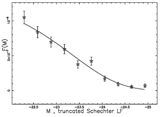
Figure 4. The observed LF for QSOs, empty stars with error bar, and the fit by the truncated Schechter LF when z$[0.3,0.5]$ and M$[-24.93,-22]$.

For the sake of comparison, Table 2 reports the three parameters of the Schechter LF.

Table 2. Parameters of the Schechter LF in the range $[0.3,0.5]$ when k = 3 and n = 10.

${\mathit{M}}^{*}$	${\mathit{\Psi }}^{*}$	$\mathit{\alpha }$	${\mathit{\chi }}^2$	${\mathit{\chi }}_{\mathit{red}}^2\mathbf{B}$	Q	AIC
–23.75	8.85 × ${10}^{-7}$	–1.37	–10.49	1.49	0.162	16049

As a first reference, the fit with the double power LF (see Equation (32)), is displayed in Figure 5 with parameters as in Table 3.

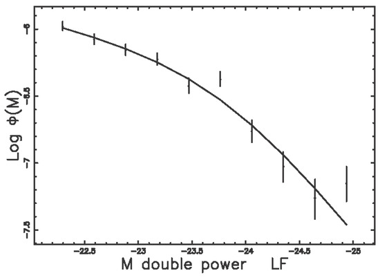
Figure 5. The observed LF for QSOs, empty stars with error bars, and the fit by the double power LF when the redshifts cover the range $[0.3,0.5]$

Table 3. Parameters of the double power LF in the range of redshifts $[0.3,0.5]$ when n = 10 and k = 4.

${\mathit{M}}^{*}$	${\mathit{\varphi }}^{*}$	$\mathit{\alpha }$	$\mathit{\beta }$	${\mathit{\chi }}^2$	${\mathit{\chi }}_{\mathit{red}}^2$	Q	AIC
–23.82	5.44 × ${10}^{-7}$	–3.57	–1.48	9.44	1.57	0.15	17.44

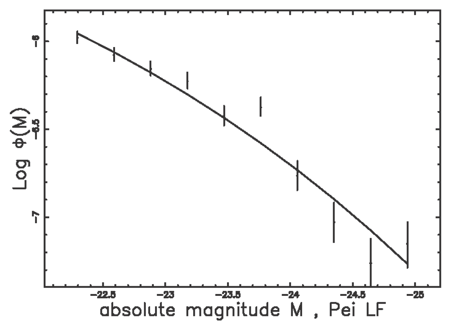
As a second reference, the fit with the Pei LF (see Equation (34)), is displayed in Figure 6 with parameters as in Table 3.

Figure 6. The observed LF for QSOs, empty stars with error bar, and the fit by the Pei LF when the redshifts cover the range $[0.3,0.5]$.

4.4. Evolutionary Effects

In order to model the evolutionary effects, an empirical variable lower bound in absolute magnitude, $M_l$, has been introduced:

$$M_l\left(z\right)=-24.5-10\times {log}_{10}(1+z)+K\left(z\right).$$

(42)

The above empirical formula is classified as a top line in Figure 5 of [28] and connected with the limits in magnitude. Conversely, the upper bound, $M_u$, was already fixed by the nonlinear Equation (37). A second evolutionary correction is

$$M^{*}=M_u\left(z\right)-0.5,$$

(43)

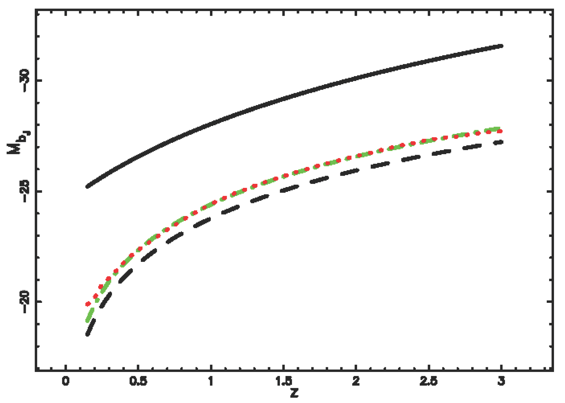
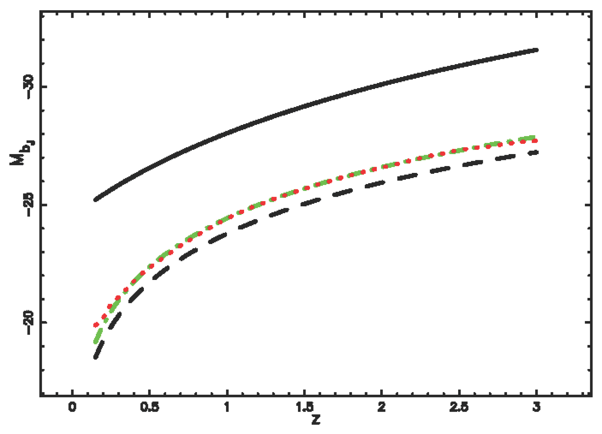
where $M_u\left(z\right)$ has been defined in Equation (37). Figure 7 reports a comparison between the theoretical and the observed average absolute magnitudes; the value of $M^{*}$ reported in Equation (43) minimizes the difference between the two curves.

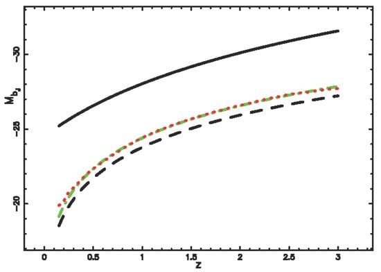
Figure 7. Average observed absolute magnitude versus redshift for QSOs (red points), average theoretical absolute magnitude for truncated Schechter LF as given by Equation (30) (dot-dash-dot green line), theoretical curve for the empirical lowest absolute magnitude at a given redshift, see Equation (42) (full black line) and the theoretical curve for the highest absolute magnitude at a given redshift (dashed black line), see Equation (37), RSS = 1.212.

As a first reference, Figure 8 reports a comparison between the theoretical and the observed average absolute magnitudes in the case of the double power LF—the value of $M^{*}$, which minimizes the difference between the two curves

$$M^{*}=M_u\left(z\right)-0.4,$$

(44)

and other parameters as in Table 3.

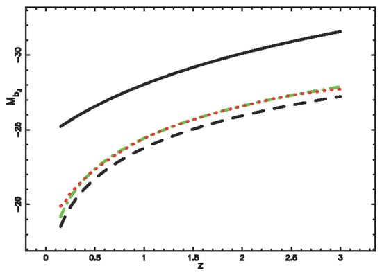
Figure 8. Average observed absolute magnitude versus redshift for QSOs (red points), average theoretical absolute magnitude for the double power LF as evaluated numerically (dot-dash-dot green line), theoretical curve for the empirical lowest absolute magnitude at a given redshift, see Equation (42) (full black line) and the theoretical curve for the highest absolute magnitude at a given redshift (dashed black line), see Equation (37), RSS = 1.138.

As a second reference, Figure 9 reports a comparison between the theoretical and the observed average absolute magnitude in the case of the Pei LF with parameters as in Table 4.

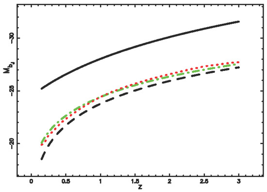
Figure 9. Average observed absolute magnitude versus redshift for QSOs (red points), average theoretical absolute magnitude for the Pei LF as evaluated numerically (dot-dash-dot green line), theoretical curve for the empirical lowest absolute magnitude at a given redshift, see Equation (42) (full black line) and the theoretical curve for the highest absolute magnitude at a given redshift (dashed black line), see Equation (37), RSS = 5.41.

Table 4. Parameters of the Pei LF in the range of redshifts $[0.3,0.5]$ with k = 3 and n = 10.

${\mathit{M}}^{*}$	${\mathit{\varphi }}^{*}$	$\mathit{\beta }$	${\mathit{\chi }}^2$	${\mathit{\chi }}_{\mathit{red}}^2$	Q	AIC
–16.47	3.68 × ${10}^{-5}$	0.924	14.4	2.05	0.044	20.40

In the above fit, the evolutionary correction for $M^{*}$ is absent.

4.5. The Photometric Maximum

The definition of the flux, f, is

$$f=\frac{L}{4\pi r^2},$$

(45)

where r is the luminosity distance. The redshift is approximated as

$$z=z_{2,1},$$

(46)

where $z_{2,1}$ has been introduced into Equation (9). The relation between $dr$ and $dz$ is

$$dr=\frac{\left(2626.1z+821.99z^2+804.33\right)}{{\left(0.44404+0.27797z\right)}^2}dz,$$

(47)

where r has been defined as $d_{L,2,1}$ by the minimax rational approximation, see Equation (8). The joint distribution in z and f for the number of galaxies is

$$\frac{dN}{d\Omega dzdf}=\frac{1}{4\pi }{\int }_0^{\infty }4\pi r^{2}dr{S}_T(L;{\mathrm{\Psi }}^{*},\alpha ,L^{*},L_l,L_u)\delta \left(z-\left(z_{2,1}\right)\right)\delta (f-\frac{L}{4\pi r^2}),$$

(48)

where $\delta$ is the Dirac delta function and $S_T(L;{\mathrm{\Psi }}^{*},\alpha ,L^{*},L_l,L_u)$ has been defined in Equation (23). The above formula has the following explicit version

$$\frac{dN}{d\Omega dzdf}=\frac{NL}{DL},$$

(49)

where

$$\begin{array}{cc}\hfill NL=& -1.71174\times {10}^{21}{\left(z+0.61116\right)}^4{\left(z+0.00227\right)}^4\hfill \\ & \times {\left(1.422{10}^9\frac{f{\left(z+0.61116\right)}^2{\left(z+0.00227\right)}^2}{{\left(z+1.59739\right)}^2{\mathit{L}}^{*}}\right)}^{\alpha }{\mathrm{e}}^{-1.422{10}^9\frac{f{\left(z+0.61116\right)}^2{\left(z+0.00227\right)}^2}{{\left(z+1.59739\right)}^2{\mathit{L}}^{*}}}\hfill \\ & \times {\Psi }^{*}\mathrm{\Gamma }\left(\alpha +1\right)\left(z+2.85165\right)\left(z+0.343138\right),\hfill \end{array}$$

(50)

where

$$\begin{array}{c}\hfill DL={\left(z+1.59739\right)}^6{L}^{*}\left(\mathrm{\Gamma }\left(\alpha +1,\frac{L_u}{L^{*}}\right)-\mathrm{\Gamma }\left(\alpha +1,\frac{L_l}{L^{*}}\right)\right).\end{array}$$

(51)

The magnitude version is

$$\begin{array}{c}\hfill \frac{dN}{d\Omega dzdm}=\frac{NM}{DM},\end{array}$$

(52)

with

$$\begin{array}{cc}\hfill NM=& -1.25459\times {10}^{30}{\left(z+0.61116\right)}^4{\left(z+0.00227\right)}^4\hfill \\ & \times {\left(1.13159\times {10}^{18}\frac{{\mathrm{e}}^{0.92103M_{\odot }-0.92103m}{\left(z+0.61116\right)}^2{\left(z+0.00227\right)}^2}{{\left(z+1.59739\right)}^2{10}^{0.4M_{\odot }-0.4M^{*}}}\right)}^{\alpha }\hfill \\ & \times {\mathrm{e}}^{-1.13159\times {10}^{18}\frac{{\mathrm{e}}^{0.92103M_{\odot }-0.92103m}{\left(z+0.61116\right)}^2{\left(z+0.00227\right)}^2}{{\left(z+1.59739\right)}^2{10}^{0.4M_{\odot }-0.4M^{*}}}}\hfill \\ & \times {\Psi }^{*}\mathrm{\Gamma }\left(\alpha +1.0\right)\left(z+2.85165\right)\left(z+0.34313\right){\mathrm{e}}^{0.92103M_{\odot }-0.92103m}\hfill \end{array}$$

(53)

and

$$\begin{array}{c}\hfill DM={\left(z+1.59739\right)}^6{10}^{0.4M_{\odot }-0.4M^{*}}\times \\ \hfill \left(\mathrm{\Gamma }\left(\alpha +1,\frac{{10}^{0.4M_{\odot }-0.4M_l}}{{10}^{0.4M_{\odot }-0.4M^{*}}}\right)-\mathrm{\Gamma }\left(\alpha +1,\frac{{10}^{0.4M_{\odot }-0.4M_u}}{{10}^{0.4M_{\odot }-0.4M^{*}}}\right)\right),\end{array}$$

(54)

where m is the apparent magnitude of the catalog, and the absolute magnitudes $M_l$, $M_u$,$M^{*}$ and $M_{\odot }$ have been defined in Section 3.2. The conversion from flux, f, to apparent magnitude, m, in the above formula is obtained from the usual formula

$$f=7.95774\times {10}^8{\mathrm{e}}^{0.92103M_{\odot }-0.92103m},$$

(55)

and

$$df=-7.32935\times {10}^8{\mathrm{e}}^{0.92103M_{\odot }-0.92103m}dm.$$

(56)

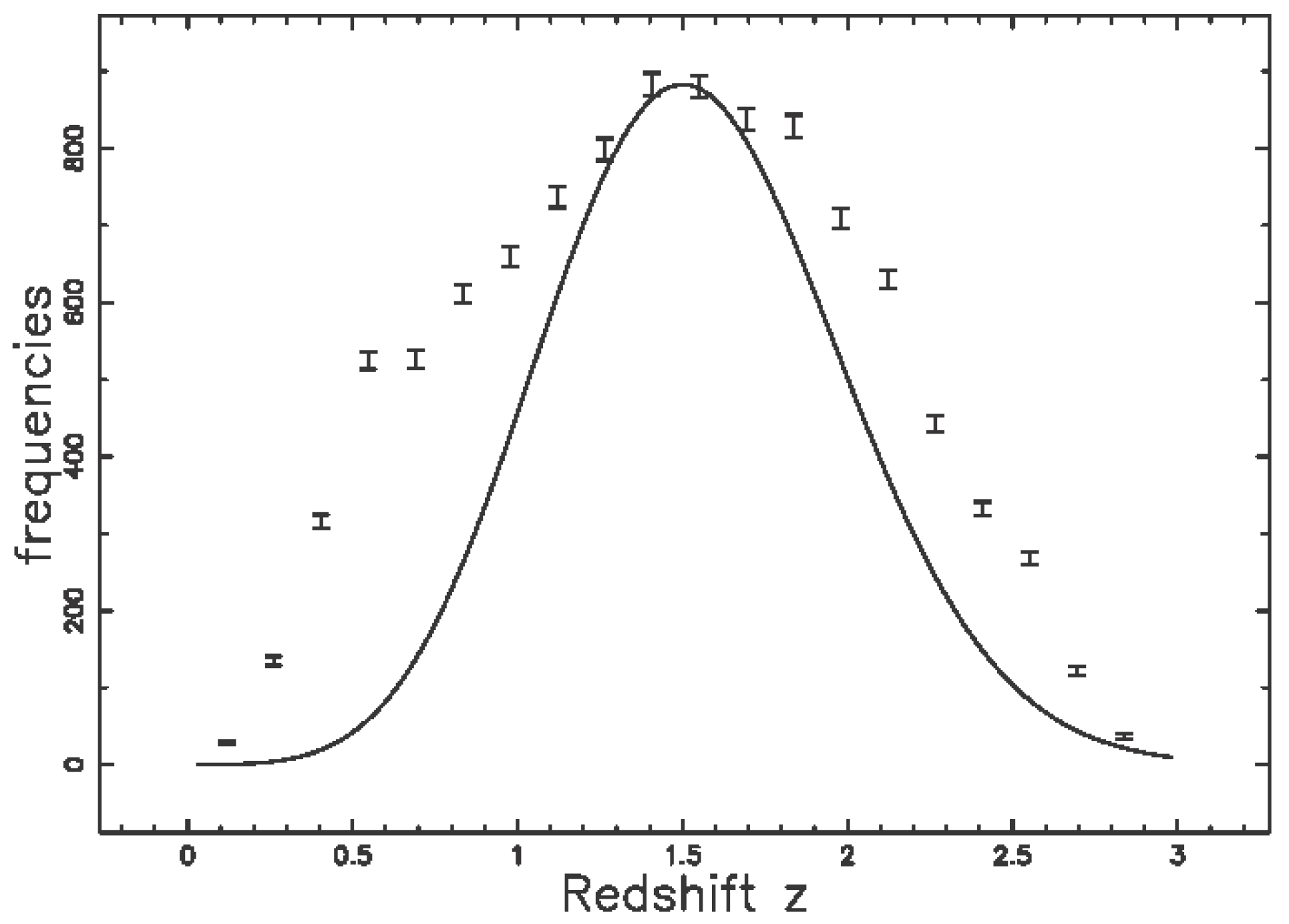
The number of galaxies in z and m, as given by formula (52), has a maximum at $z=z_{pos-max},$ but there is no analytical solution for such a position and a numerical analysis should be performed. Figure 10 reports the observed and the theoretical number of QSOs as functions of the redshift at a given apparent magnitude when $M_l\left(z\right)$ is given by Equation (42) and $M_u\left(z\right)$ is given by Equation (37). Here, we adopted the law of rare events, i.e., the Poisson distribution, in which the variance is equal to the mean, i.e., the error bar is given by the square root of the frequency.

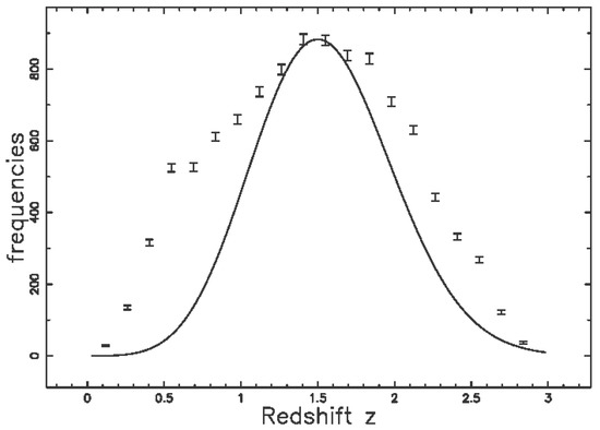
Figure 10. The QSOs with $20.16\le m\le 20.85$ are organized in frequencies versus spectroscopic redshift, points with error bars. The redshifts cover the range $[0,3]$ and the histogram’s interval is 0.14. The maximum frequency of observed QSOs is at $z=1.478$ and the number of bins is 20. The full line is the theoretical curve generated by $\frac{dN}{d\Omega dzdm}\left(z\right)$ as given by the application of the truncated Schechter LF, which is Equation (52) with parameters as in Table 1 but $M^{*}=-22.5$. The theoretical maximum is at $z=1.491$.

In the above fit, the observed position of the maximum, $z=1.478$, and the theoretical prediction, $z=1.491$, have approximately the same value. In the two regions surrounding the maximum, the degree of prediction is not as accurate, due to the fact that the three absolute magnitudes $M_l$, $M_u$ and $M^{*}$ are functions of z.

5. Conclusions

Absolute Magnitude

The evaluation of the absolute magnitude of a QSO is connected with the distance modulus, which, in the case of the flat cosmology, (${\Omega }_{\mathrm{M}}=0.3$, $H_0=70$$\mathrm{km}{\mathrm{s}}^{-1}{\mathrm{Mpc}}^{-1}$) is reported in Equation (5) as a Taylor series of order 8 with range in z, $[0-4]$. As an application of the above series, we derived an inverse formula for the redshift as a function of the luminosity distance and an approximate formula for the total comoving volume.

Truncated Schechter LF

The Schechter LF is characterized by three parameters: ${\mathrm{\Phi }}^{*}$, $\alpha$ and $M^{*}$. The truncated Schechter LF is characterized by five parameters: ${\mathrm{\Psi }}^{*}$, $\alpha$, $M^{*}$, $M_l$ and $M_u$. The reference LF for QSOs, the double power law LF, is characterized by four parameters: ${\varphi }^{*}$, $\alpha$, $\beta$ and $M^{*}$. An application of the above LFs in the range of z $[0.3,0.5]$ gives the following reduced chi-square ${\chi }_{red}^2=$ 2.57 for the truncated Schechter LF, ${\chi }_{red}^2=$ 1.49 for the Schechter LF, ${\chi }_{red}^2=$ 1.57 for the double power LF, and ${\chi }_{red}^2=$ 2.05 for the Pei LF. The other statistical such as the AIC are reported in Table 1, Table 2, Table 3 and Table 4. We can therefore speak of minimum differences between the four LFs here analyzed in the nearby universe defined by redshifts $[0.3,0.5]$.

Evolutionary effects

The evolution of the LF for QSOs as a function of the redshift is here modeled by an upper and lower truncated Schechter function. This choice allows modeling the lower bound in luminosity (the higher bound in absolute magnitude) according to the evolution of the absolute magnitude (see Equation (37)). The evaluation of the upper bound in luminosity (the lower bound in absolute magnitude) is empirical and is reported in Equation (42). A variable value of $M^{*}$ with z in the case of the truncated Schechter LF (see Equation (43)), allows matching the evolution of the observed average value of absolute magnitude with the theoretical average value of absolute magnitude (see Figure 7). A comparison is done with the theoretical average value in absolute magnitude for the case of a double power law and the Pei function (see Figure 8 and Figure 9).

Maximum in magnitude

The joint distribution in redshift and energy flux density is here modeled in the case of a flat universe, see formula 48. The position in redshift of the maximum in the number of galaxies for a given flux or apparent magnitude does not have an analytical expression and is therefore found numerically (see Figure 10). A comparison can be done with the number of galaxies as a function of the redshift in $[0-0.3]$ for the 2dF Galaxy Redshift Survey in the South and North galactic poles (see Figure 6 in [37]), where the theoretical model is obtained by the generation of random catalogs.

References

- Schechter, P. An analytic expression for the luminosity function for galaxies. Astrophys. J. 1976, 203, 297–306. [Google Scholar] [CrossRef]
- Warren, S.J.; Hewett, P.C.; Osmer, P.S. A wide-field multicolor survey for high-redshift quasars, Z greater than or equal to 2.2. 3: The luminosity function. Astrophys. J. 1994, 421, 412–433. [Google Scholar] [CrossRef]
- Goldschmidt, P.; Miller, L. The UVX quasar optical luminosity function and its evolution. Mon. Not. R. Astron. Soc. 1998, 293, 107–112. [Google Scholar] [CrossRef]
- Driver, S.P.; Phillipps, S. Is the Luminosity Distribution of Field Galaxies Really Flat? Astrophys. J. 1996, 469, 529–534. [Google Scholar] [CrossRef]
- Bell, E.F.; McIntosh, D.H.; Katz, N.; Weinberg, M.D. The Optical and Near-Infrared Properties of Galaxies. I. Luminosity and Stellar Mass Functions. Astrophys. J. Suppl. Ser. 2003, 149, 289–312. [Google Scholar] [CrossRef]
- Blanton, M.R.; Lupton, R.H.; Schlegel, D.J.; Strauss, M.A.; Brinkmann, J.; Fukugita, M.; Loveday, J. The Properties and Luminosity Function of Extremely Low Luminosity Galaxies. Astrophys. J. 2005, 631, 208–230. [Google Scholar] [CrossRef]
- Alcaniz, J.S.; Lima, J.A.S. Galaxy Luminosity Function: A New Analytic Expression. Braz. J. Phys. 2004, 34, 455–458. [Google Scholar] [CrossRef]
- Croom, S.M.; Smith, R.J.; Boyle, B.J.; Shanks, T.; Miller, L.; Outram, P.J.; Loaring, N.S. The 2dF QSO Redshift Survey—XII. The spectroscopic catalogue and luminosity function. Mon. Not. R. Astron. Soc. 2004, 349, 1397–1418. [Google Scholar] [CrossRef]
- Coffey, C.S.; Muller, K.E. Properties of doubly-truncated gamma variables. Commun. Stat. Theory Methods 2000, 29, 851–857. [Google Scholar] [CrossRef] [PubMed]
- Zaninetti, L. The Luminosity Function of Galaxies as Modeled by a Left Truncated Beta Distribution. Int. J. Astron. Astrophys. 2014, 4, 145–154. [Google Scholar] [CrossRef]
- Zaninetti, L. On the Number of Galaxies at High Redshift. Galaxies 2015, 3, 129–155. [Google Scholar] [CrossRef]
- Zaninetti, L. Pade Approximant and Minimax Rational Approximation in Standard Cosmology. Galaxies 2016, 4, 4. [Google Scholar] [CrossRef]
- Boyle, B.J.; Shanks, T.; Peterson, B.A. The evolution of optically selected QSOs. II. Mon. Not. R. Astron. Soc. 1988, 235, 935–948. [Google Scholar] [CrossRef]
- Pei, Y.C. The luminosity function of quasars. Astrophys. J. 1995, 438, 623–631. [Google Scholar] [CrossRef]
- Adachi, M.; Kasai, M. An Analytical Approximation of the Luminosity Distance in Flat Cosmologies with a Cosmological Constant. Prog. Theor. Phys. 2012, 127, 145–152. [Google Scholar] [CrossRef]
- Mészáros, A.; Řípa, J. A curious relation between the flat cosmological model and the elliptic integral of the first kind. Astron. Astrophys. 2013, 556, A13. [Google Scholar] [CrossRef]
- Etherington, I.M.H. On the Definition of Distance in General Relativity. Philos. Mag. 1933, 15, 761. [Google Scholar] [CrossRef]
- Press, W.H.; Teukolsky, S.A.; Vetterling, W.T.; Flannery, B.P. Numerical Recipes in FORTRAN. The Art of Scientific Computing; Cambridge University Press: Cambridge, UK, 1992. [Google Scholar]
- Akaike, H. A new look at the statistical model identification. IEEE Trans. Autom. Control 1974, 19, 716–723. [Google Scholar] [CrossRef]
- Liddle, A.R. How many cosmological parameters? Mon. Not. R. Astron. Soc. 2004, 351, L49–L53. [Google Scholar] [CrossRef]
- Godlowski, W.; Szydowski, M. Constraints on Dark Energy Models from Supernovae. In 1604-2004: Supernovae as Cosmological Lighthouses; Turatto, M., Benetti, S., Zampieri, L., Shea, W., Eds.; Astronomical Society of the Pacific Conference Series; Astronomical Society of the Pacific: San Francisco, CA, USA, 2005; Volume 342, pp. 508–516. [Google Scholar]
- Olver, F.W.J.; Lozier, D.W.; Boisvert, R.F.; Clark, C.W. NIST Handbook of Mathematical Functions; Cambridge University Press: Cambridge, UK, 2010. [Google Scholar]
- Boyle, B.J.; Shanks, T.; Croom, S.M.; Smith, R.J.; Miller, L.; Loaring, N.; Heymans, C. The 2dF QSO Redshift Survey—I. The optical luminosity function of quasi-stellar objects. Mon. Not. R. Astron. Soc. 2000, 317, 1014–1022. [Google Scholar] [CrossRef]
- Richards, G.T.; Strauss, M.A.; Fan, X.; Hall, P.B.; Jester, S.; Schneider, D.P.; Vanden Berk, D.E.; Stoughton, C.; Anderson, S.F.; Brunner, R.J.; et al. The Sloan Digital Sky Survey Quasar Survey: Quasar Luminosity Function from Data Release 3. Astron. J. 2006, 131, 2766–2787. [Google Scholar] [CrossRef]
- Ross, N.P.; McGreer, I.D.; White, M.; Richards, G.T.; Myers, A.D.; Palanque-Delabrouille, N.; Strauss, M.A.; Anderson, S.F.; Shen, Y.; Brandt, W.N.; et al. The SDSS-III Baryon Oscillation Spectroscopic Survey: The Quasar Luminosity Function from Data Release Nine. Astrophys. J. 2013, 773, 14. [Google Scholar] [CrossRef]
- Singh, S.A. Optical Luminosity Function of Quasi Stellar Objects. Am. J. Astron. Astrophys. 2016, 4, 78. [Google Scholar] [CrossRef]
- Wisotzki, L. Quasar spectra and the K correction. Astron. Astrophys. 2000, 353, 861–866. [Google Scholar]
- Croom, S.M.; Richards, G.T.; Shanks, T.; Boyle, B.J.; Strauss, M.A.; Myers, A.D.; Nichol, R.C.; Pimbblet, K.A.; Ross, N.P.; Schneider, D.P.; et al. The 2dF-SDSS LRG and QSO survey: The QSO luminosity function at z between 0.4 and 2.6. Mon. Not. R. Astron. Soc. 2009, 399, 1755–1772. [Google Scholar] [CrossRef]
- Malmquist, K. A study of the stars of spectral type A. Lund Medd. Ser. II 1920, 22, 1–10. [Google Scholar]
- Malmquist, K. On some relations in stellar statistics. Lund Medd. Ser. I 1922, 100, 1–10. [Google Scholar]
- Behr, A. Zur Entfernungsskala der extragalaktischen Nebel. Astron. Nachr. 1951, 279, 97–107. [Google Scholar] [CrossRef]
- Page, M.J.; Carrera, F.J. An improved method of constructing binned luminosity functions. Mon. Not. R. Astron. Soc. 2000, 311, 433–440. [Google Scholar] [CrossRef]
- Avni, Y.; Bahcall, J.N. On the simultaneous analysis of several complete samples—The V/Vmax and Ve/Va variables, with applications to quasars. Astrophys. J. 1980, 235, 694–716. [Google Scholar] [CrossRef]
- Eales, S. Direct construction of the galaxy luminosity function as a function of redshift. Astrophys. J. 1993, 404, 51–62. [Google Scholar] [CrossRef]
- Ellis, R.S.; Colless, M.; Broadhurst, T.; Heyl, J.; Glazebrook, K. Autofib Redshift Survey—I. Evolution of the galaxy luminosity function. Mon. Not. R. Astron. Soc. 1996, 280, 235–251. [Google Scholar] [CrossRef]
- Yuan, Z.; Wang, J. A graphical analysis of the systematic error of classical binned methods in constructing luminosity functions. Astrophys. Space Sci. 2013, 345, 305–313. [Google Scholar] [CrossRef]
- Cole, S.; Percival, W.J.; Peacock, J.A.; Norberg, P.; Baugh, C.M.; Frenk, C.S.; Baldry, I.; Bland-Hawthorn, J.; Bridges, T.; Cannon, R.; et al. The 2dF Galaxy Redshift Survey: power-spectrum analysis of the final data set and cosmological implications. Mon. Not. R. Astron. Soc. 2005, 362, 505–534. [Google Scholar] [CrossRef]