This section reviews the four broken power law distribution and the lognormal distribution and derives an analytical expression for the number of GRBs for a given flux in the linear and non-linear cases.
3.2. Lognormal Distribution
Let
L be a random variable taking values
L in the interval
; the lognormal probability density function (PDF), following [
12] or formula (14.2)
in [
13], is:
where
and
. The mean luminosity is:
and the variance,
, is:
The distribution function (DF) is:
where
is the error function; see [
14]. A luminosity function for GRB,
, can be obtained by multiplying the lognormal PDF by
, which is the number of GRB per unit volume, Mpc
units for unit time, y units,
A numerical value for the constant
can be obtained by dividing the number of GRBs,
, observed in a time,
T, in a given volume
V by the volume itself and by
T, which is the time over which the phenomena are observed, in the case of SWIFT-BAT, 70 months; see [
1],
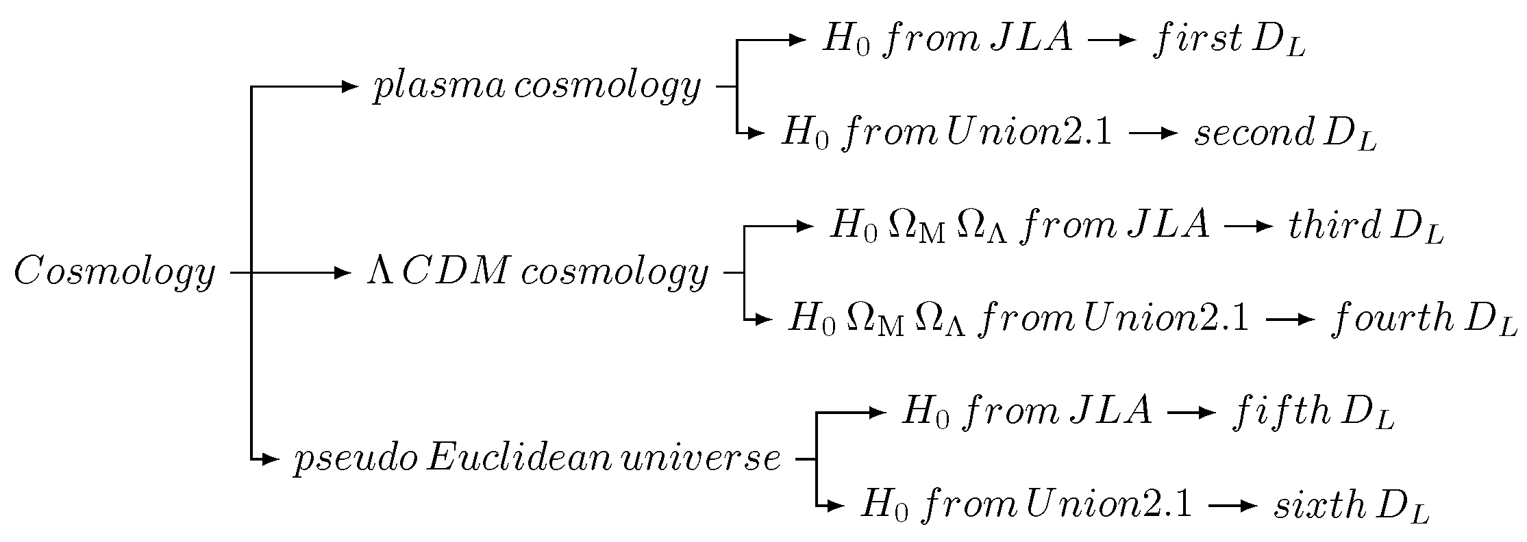
where the volume is different in the three cosmologies,
where
has been defined in Equation (
10). The parameters of the fit for the four broken power law’s PDF are reported in
Table 6 when the luminosity is taken with the
correction;
Figure 5.
The parameters of the fit for the lognormal PDF are reported in
Table 7 when the luminosity is taken with the
correction.
The case of LF modeled by a lognormal PDF with
L as represented by a monochromatic luminosity in the X-band (14–195 keV) is reported in
Table 8.
The goodness of the fit with the lognormal PDF has been assessed by applying the Kolmogorov–Smirnov (K–S) test [
15,
16,
17]. The K–S test, as implemented by the FORTRAN subroutine KSONE in [
18], finds the maximum distance,
D, between the theoretical and the observed DF, as well as the significance level,
; see Formulas 14.3.5 and 14.3.9 in [
18]; the values of
indicate that the fit is acceptable; see
Table 7 for the results.
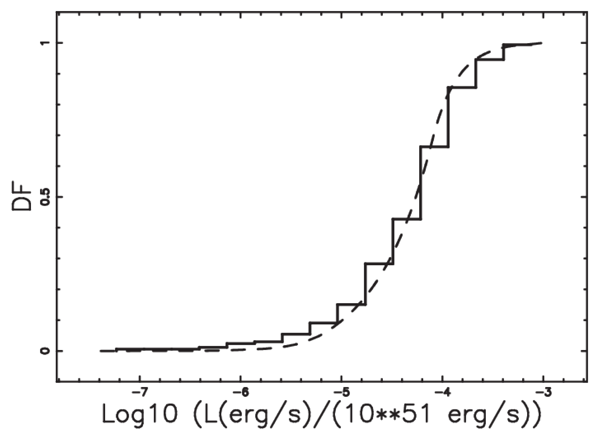
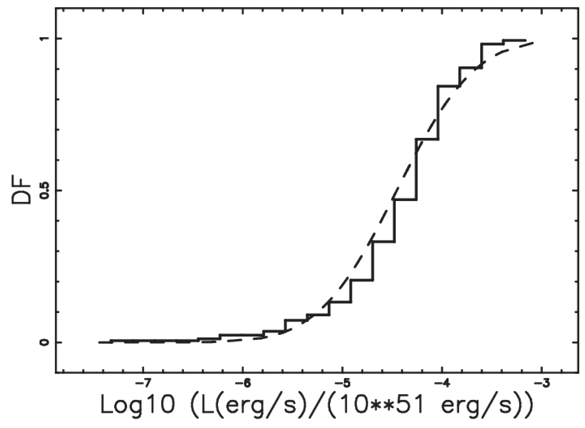
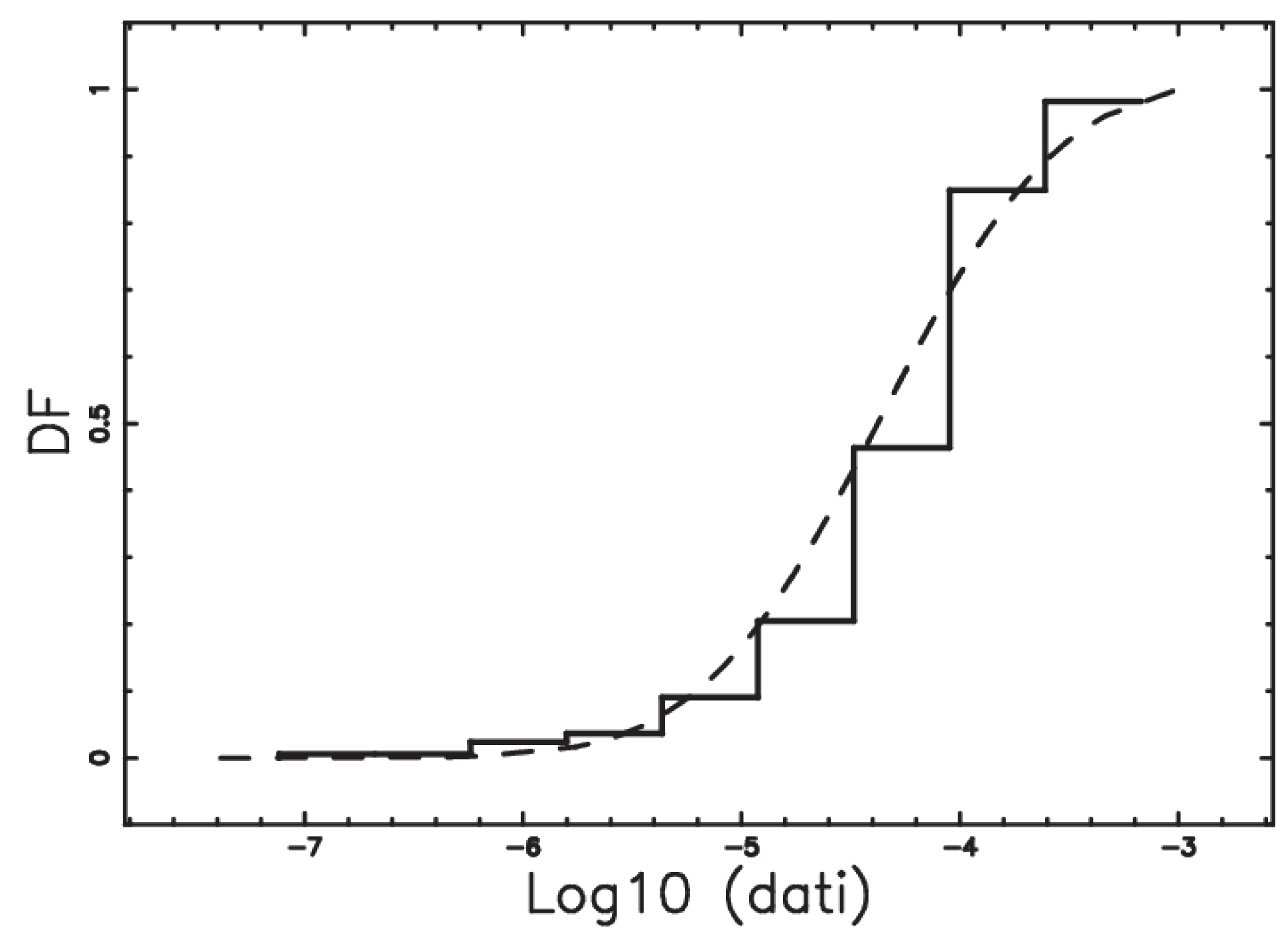
In the case of the ΛCDM cosmology,
Figure 6 reports the lognormal DF, with the parameters as in
Table 7.
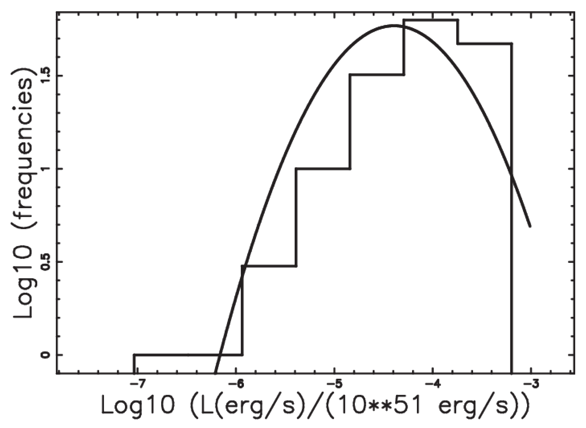
In the case of the ΛCDM cosmology,
Figure 7 reports a comparison between the empirical distribution and the lognormal PDF, and
Figure 6 reports the lognormal DF, with the parameters as in
Table 7.
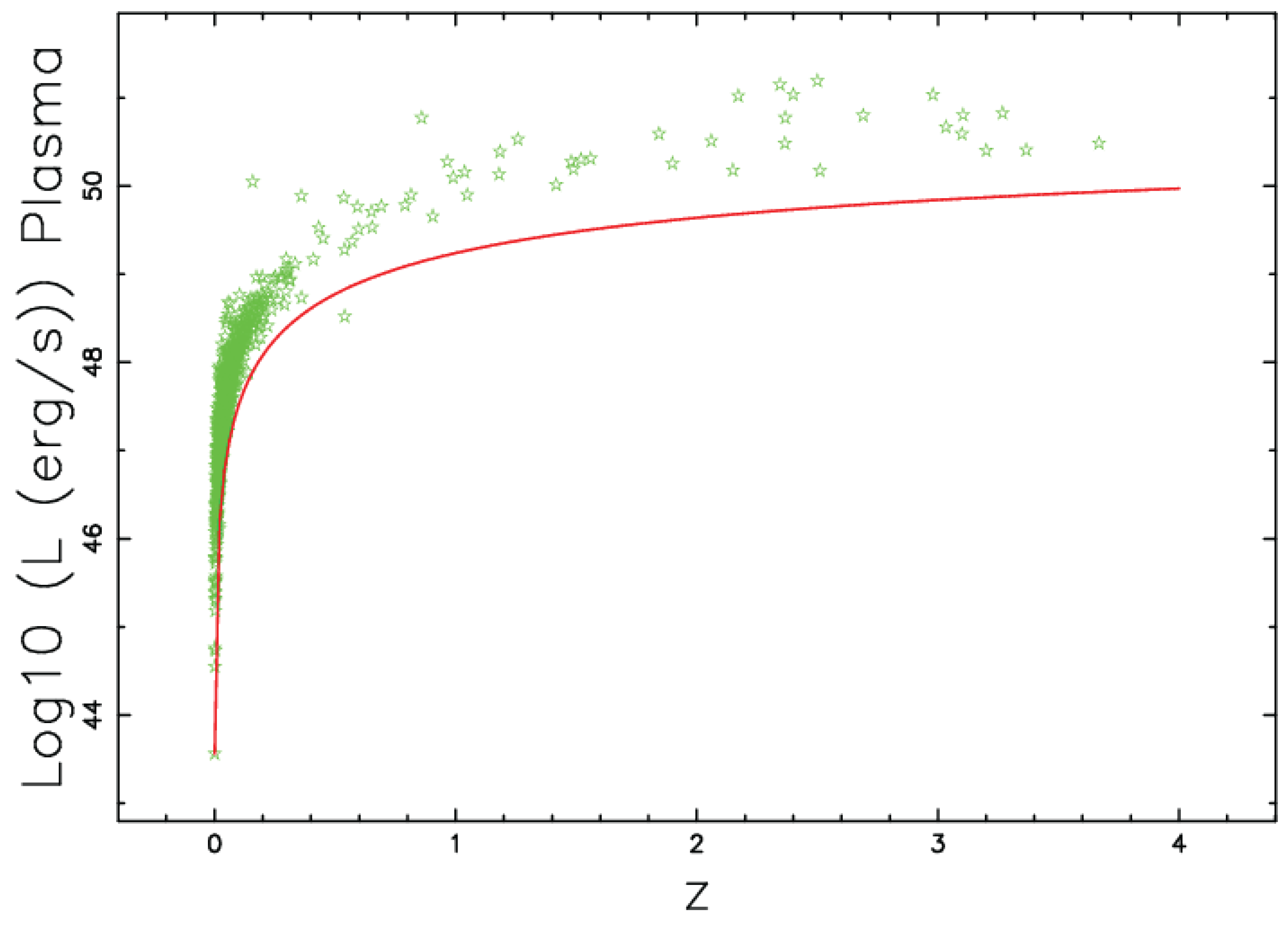
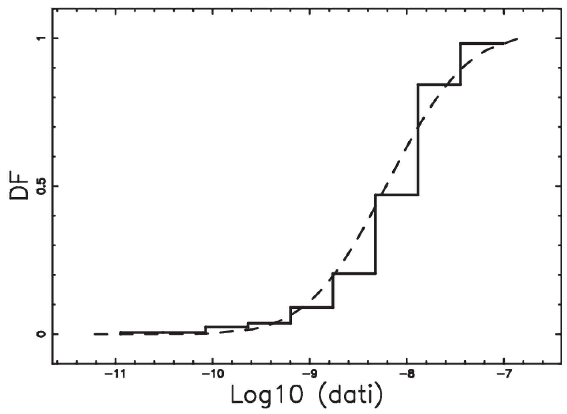
The case of the plasma and pseudo-Euclidean cosmologies is covered in
Figure 8 and
Figure 9, respectively.
3.3. The Linear Case
We assume that the flux,
f, scales as
, according to Equation (
15):
and:
The relation between the two differentials
and
is:
The joint distribution in
z and
f for the number of galaxies is:
where
δ is the Dirac delta function. We now introduce the critical value of
z,
, which is:
The evaluation of the integral over luminosities and distances gives:
where
,
and
represent the differential of the solid angle, the redshift and the flux, respectively, and
is the normalization of the lognormal LF for GRB. The number of GRBs in
z and
f as given by the above formula has a maximum at
, where:
which can be re-expressed as:
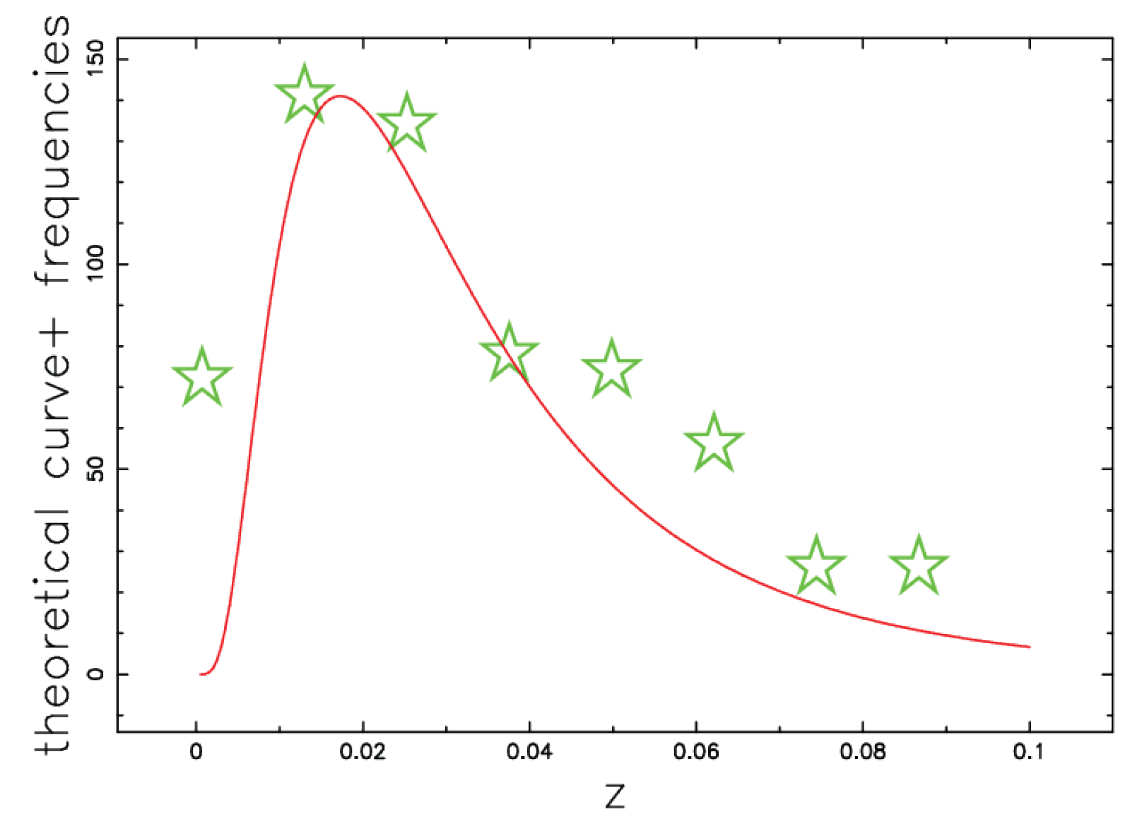
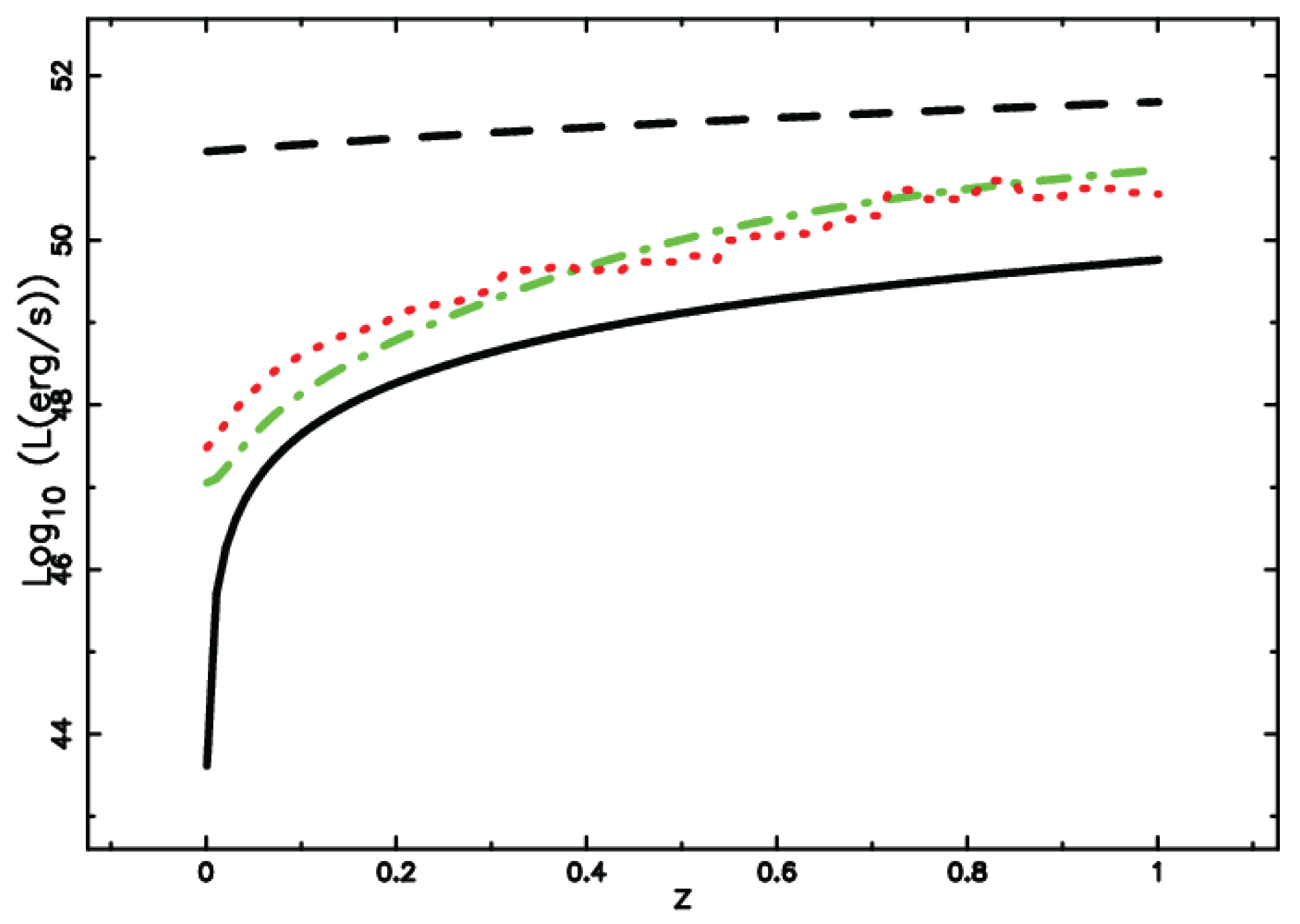
Figure 10 reports the observed and theoretical number of GRBs with a given flux as a function of the redshift.
The theoretical maximum as given by Equation (
35) is at
, with the parameters as in
Table 7, against the observed
. The theoretical mean redshift of GRBs with flux
f can be deduced from Equation (
34):
The above integral does not have an analytical expression and should be numerically evaluated. The above formula with parameters as in
Figure 10 gives a theoretical/numerical
against the observed
. The quality of the fit in the number of GRBs with a given flux depends on the chosen flux, the interval of the flux in which the frequencies are evaluated and the number of histograms. A larger number of available GRBs will presumably increase the goodness of the fit.
3.4. The Non-Linear Case
We assume that
and:
where
r is the distance; in our case,
d is as represented by the non-linear Equation (
11). The relation between
and
is:
The joint distribution in
z and
f for the number of galaxies is:
where
δ is the Dirac delta function.
The evaluations of the integral over luminosities and distances give:
The above formula has a maximum at
, where:
where
is the Lambert
W function; see [
14]. The above maximum can be re-expressed as:
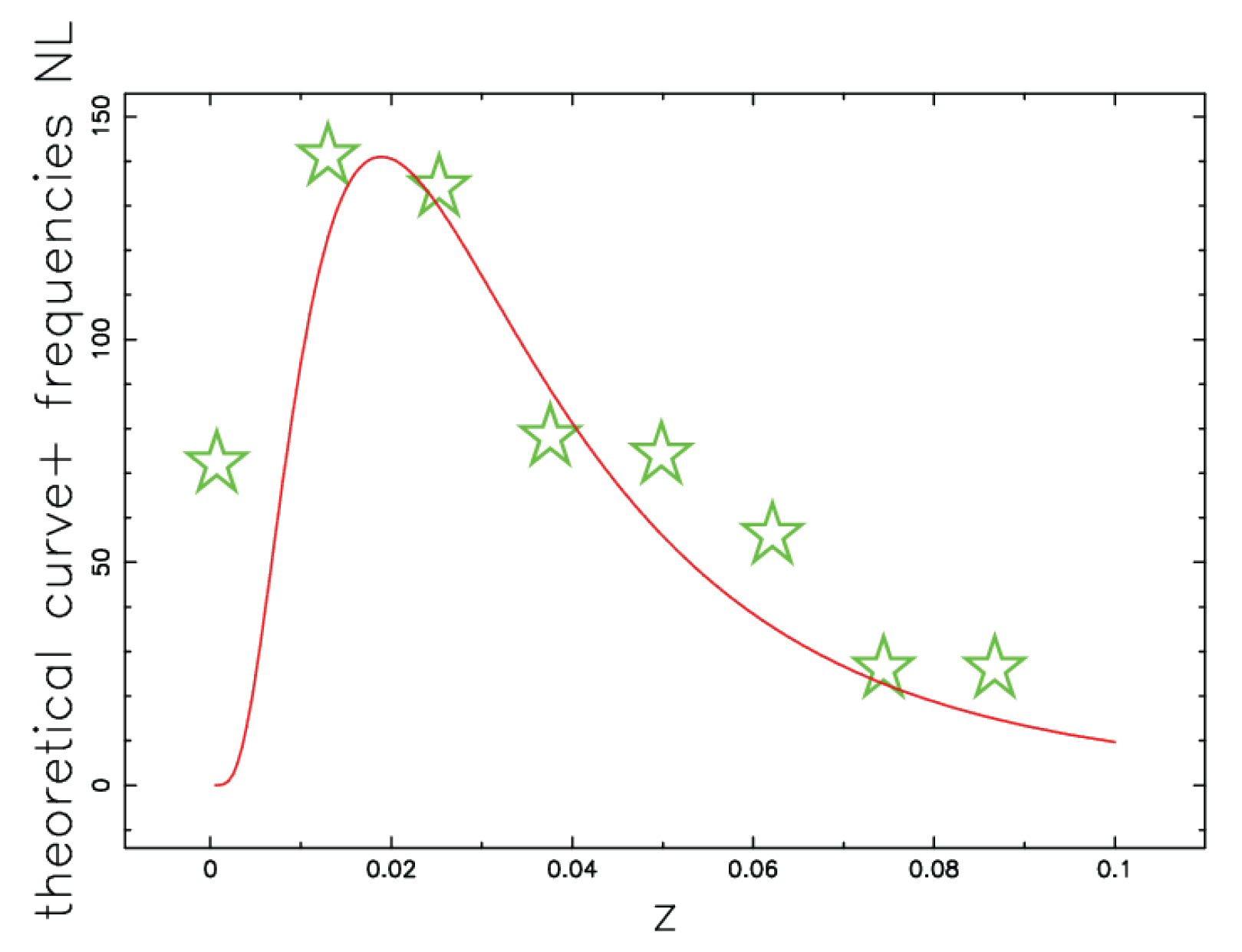
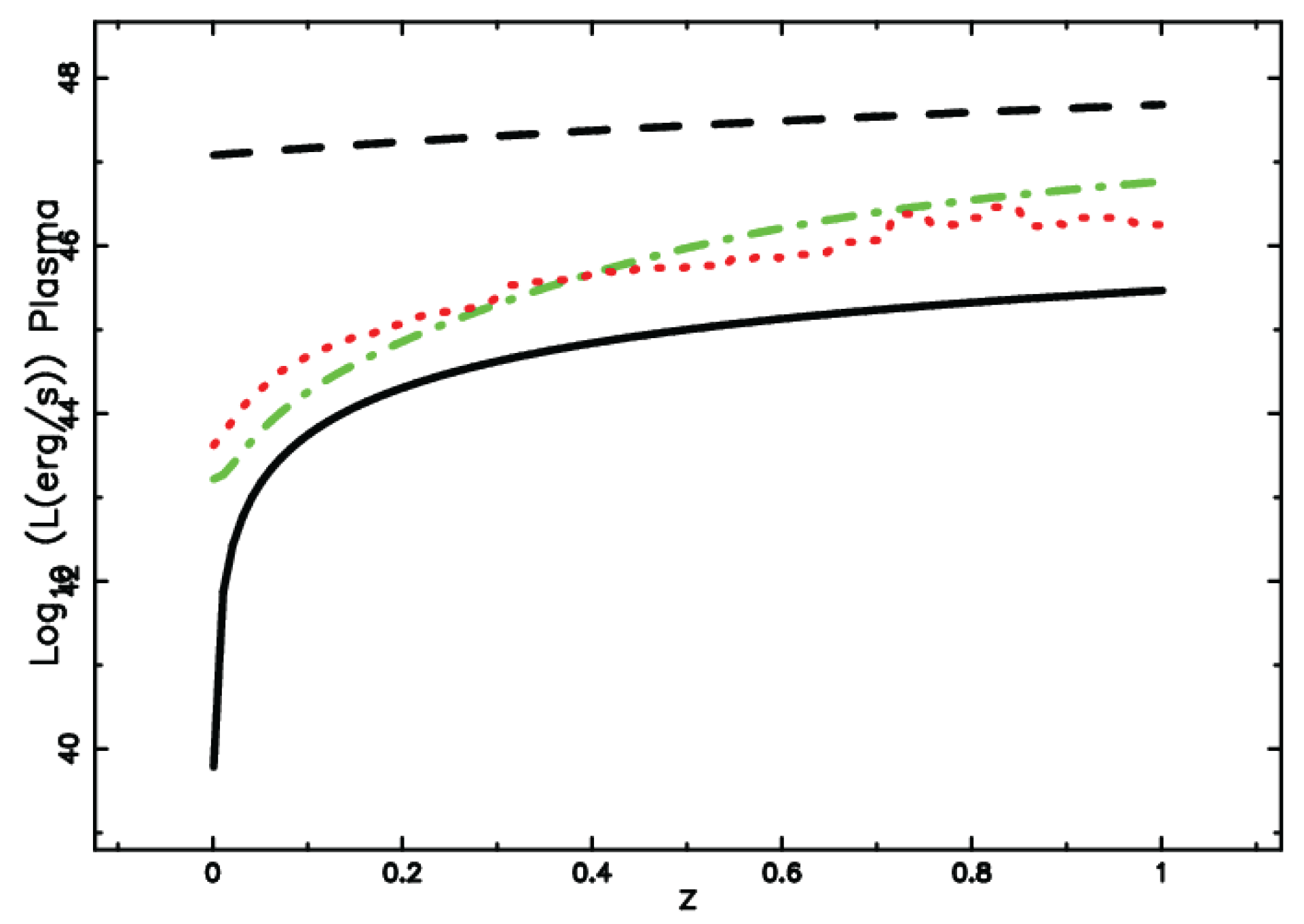
Figure 11 reports the observed and theoretical number of GRBs with a given flux as a function of the redshift.
In the case of the plasma cosmology, the theoretical maximum as given by Equation (
42) is at
, with the parameters as in
Table 7, against the observed
. The theoretical averaged redshift of GRBs is
against the observed
.


