The VLBA-BU-BLAZAR Multi-Wavelength Monitoring Program

Abstract

We describe a multiwavelength program of monitoring of a sample of bright γ-ray blazars, which the Boston University (BU) group has being carrying out since June 2007. The program includes monthly monitoring with the Very Long Baseline Array at 43 GHz, optical photometric and polarimetric observations, construction and analysis of UV and X-ray light curves obtained with the Rossi X-ray Timing Explorer (RXTE) and Swift satellites, and construction and analysis of γ-ray light curves based on data provided by the Large Area Telescope of the Fermi Gamma-ray Space Telescope. We present general results about the kinematics of parsec-scale radio jets, as well as the connection between γ-ray outbursts and jet events.

1. Introduction

During the Compton Gamma Ray Observatory operation from 1991 to 2000, the Energetic Gamma Ray Experiment Telescope (EGRET) detected nearly 70 blazars at photon energies of 0.1–3 GeV [1]. EGRET was a predecessor of the Large Area Telescope (LAT) of the Fermi Gamma-Ray Space Telescope [2], which was launched in August 2008 and continues to operate at 0.1–300 GeV in survey mode. The Fermi LAT has already detected 1563 active galactic nuclei (AGNs), 98% of which are blazars [3]. The most common explanation of the γ-ray emission in blazars in the 1990s, (e.g., [4]), which continues to prevail in the Fermi era, (e.g., [5,6]), is that γ-rays originate close to the black hole (BH), within the broad line region (BLR). This is based on short timescales of variability and an ideal pool of external optical/UV seed photons available from the BLR for inverse Compton scattering up to γ-ray energies. In the EGRET era, the Boston University (BU) blazar group performed a monitoring program of the milliarcsecond-scale structure of γ-ray bright blazars (42 sources) with the Very Long Baseline Array (VLBA) at 22 and 43 GHz, and found a statistically significant correlation between the flux density of the VLBI core and the γ-ray flux and higher apparent speeds in γ-ray blazars [7] than in radio-loud AGNs studied in the Caltech-Jodrell Bank flat-spectrum source survey (CJF, [8]). These results were confirmed with higher statistical significance in the Fermi era [9,10]. In addition, the BU group examined the coincidence of times of high γ-ray flux and ejections of superluminal components from the core and, despite sparse EGRET γ-ray light curves, found that in ∼50% of events with sufficient VLBA and γ-ray data, γ-ray outbursts can be associated with the appearance of superluminal knots in radio jets [11]. This finding suggested that the γ-ray flares occurred in the parsec-scale regions of the jet rather than closer to the central engine. However, only 23 events had sufficient EGRET and VLBA data, and the times of superluminal knot ejections were determined with large uncertainties. Here, we describe a comprehensive multi-wavelength program which the BU blazar group has been carrying out in the Fermi era. The program aims to determine the locations and mechanisms of origin of high energy photons in blazars.

2. Sample and Observations

In June 2007, the Boston University blazar group started a large program of multi-wavelength observations of a sample of bright γ-ray blazars (the VLBA-BU-BLAZAR program). The initial sample included 30 blazars detected as bright γ-ray sources by EGRET, with radio flux density at 43 GHz exceeding 0.5 Jy, declination >−30${}^{\circ }$, and optical magnitude in R band <18.5${}^m$. In 2009, after the first catalog of γ-ray sources detected by the Fermi LAT during the first year of operation was issued [12], we added 6 more sources, mostly objects of BL Lac type, and in 2012 we included the famous TeV blazar Mrk501 in our study. Currently, the sample consists of 21 flat radio spectrum quasars (FSRQs), 13 BL Lac objects (BLLacs), and 3 radio galaxies (RGs). This is a flux limited sample at radio, optical, and γ-ray wavelengths, with strong variability expected across the electromagnetic spectrum and in the parsec-scale jet structure. Among the sample sources, 7 BL Lac objects and 3 quasars have been detected at TeV energies. The redshifts in the sample range from 0.0177 to 2.17.

2.1. VLBA Monitoring

The focal point of our program is monthly monitoring of the sample with the VLBA at 43 GHz. Observations are performed in 24 h sessions with 30–32 objects per session and 8–10 scans of ∼5 min duration for each source, in both left and right circular polarization. In addition we have performed 8 campaigns with 3 epochs of VLBA observations during 2 weeks each to search for short-timescale variability in the parsec-scale jets. Each session of these campaigns had a 16-h duration and observed 16 sources from our sample. All data are correlated at the National Radio Astronomy Observatory (NRAO) correlator in Socorro (NM, USA), and reduced at Boston University using the Astronomical Image Processing System (AIPS), supported by NRAO, and the software package Difmap, developed at the California Institute of Technology. Here we will discuss mostly the data obtained from June 2007 to January 2013, which were reduced and modelled in the same manner as described in [13]. During this period we obtained 76 epochs of total and polarized intensity images of the γ-ray blazars, which can be found at our website: www.bu.edu/blazars/VLBAproject.html.

2.2. Gamma-Ray Light Curves

For each source in our sample we calculate a γ-ray light curve with a 7 day integration time using photon and spacecraft data provided by the Fermi LAT. The light curves have been recalculated for new releases of the Fermi LAT data and software versions. The γ-ray light curves, which are currently presented at our website and will be discussed in this paper, have been calculated using the Pass 8 data and software version v10r0p5, released 24 June 2015, with diffuse source models gll_iem_v06 and iso_P8R2_SOURCE_V6_v06. The calculations have been performed with fixed spectral characteristics corresponding to those listed in the third Fermi LAT catalog of γ-ray sources [3] for all sources within 15${}^{\prime \prime }$ radius of a blazar, except for the flux normalization parameter of the blazar and brightest γ-ray sources in its neighborhood. However, during high γ-ray activity states the γ-ray fluxes are calculated with a binning size of 1–3 days and with the spectral characteristics of the blazar allowed to vary.

2.3. Optical Observations

From January 2007 to January 2016, we carried out 517 nights of optical observations at the 1.83 m Perkins telescope using the PRISM camera (www.bu.edu/prism/) in R band polarimetric mode and BVRI photometric modes, although 26 nights do not have usable data due to either weather conditions or technical problems. For each source we obtain 3–5 series of measurements at 0${}^{\circ }$, 90${}^{\circ }$, 45${}^{\circ }$, and 135${}^{\circ }$ positions of the polaroid to derive Stokes I, Q, and U parameters. We use polarized standard stars from [14] to correct for an instrumental shift of the position angle (PA) of polarization with respect to the world coordinate system defined as following: the PA of north is equal to 0${}^{\circ }$ and the PA of east is +90${}^{\circ }$. The instrumental polarization of the PRISM camera is low, 0.3%–0.5%, and we correct for this using stars in the field of the blazar, assuming that field stars are not polarized. This removes the contribution of interstellar polarization as well. Information for comparison stars, which we use to perform BVRI photometry of the sources in our sample, can be found either at the St. Petersburg University Observatory (Russia) website (lacerta.astro.spbu.ru/program) or at the MAPCAT (Monitoring AGN with Polarimetry at the Calar Alto Telescope project, Spain) website (www.iaa.es/~iagudo/research/MAPCAT/source_list/list.html). Both of these projects include our sample in their polarimetric and photometric monitoring. We combine our polarimetric and photometric data with observations obtained by the St.Petersburg University AGN group and MAPCAT project as well as with observations carried out by Dr. P. Smith at Steward Observatory (james.as.arizona.edu/~psmith/Fermi/#mark2; see also his paper in these proceedings). Curves of R band photometric and polarimetric (degree of polarization, P, and PA, χ) measurements vs. time obtained for each source in the sample by the BU blazar group are shown at our website.

2.4. X-ray and UV Light Curves

We performed intense monitoring, 2–3 times per week, of several blazars in our sample with the Rossi X-ray Timing Explorer (RXTE) at 2–10 keV up to its decommissioning on 5 January 2012. An example of the RXTE data reduction is given, e.g., in [15]. In 2009 the Swift X-ray Telescope (XRT) initiated irregular monitoring of a list of Fermi LAT sources (www.swift.psu.edu/monitoring) at 0.3–10 keV. We use the Swift archive and observations from our successful proposals and approved target-of-opportunity (ToO) programs with Swift to construct X-ray and UV light curves. We perform the Swift UVOT and XRT data reduction in the same manner as described in [16]. The XRT light curves are presented at our website.

2.5. Radio Light Curves

We use total flux densities at 37 GHz provided by the Metsähovi Radio Observatory (Aalto University, Espoo, Finland) to check for amplitude calibration of the VLBA data. We analyze 37 GHz light curves and light curves at 230 and 350 GHz obtained at the Submillimeter Array (Hawaii, Mauna Kea) to correlate jet events with activities in the mm-wave light curves.

3. Jet Kinematics on Parsec Scales

We have identified 289 jet features that appeared in the jets of 36 sources (21 FSRQs, 12 BLLacs, and 3 RGs) during the period from June 2007 to January 2013. We fit the total intensity visibilities with a source model consisting of a number of circular components with gaussian brightness distributions, and determine the following parameters of each component: S—flux density in Jy, r—distance from the core in milli-arcseconds (mas), Θ—position angle in degrees, and a—FWHM diameter in mas. Two components at different epochs are identified as the same feature if there is consistency in their parameters, although in some cases the identification is not unique. Based on our measurements, a feature can be classified as the VLBI core, or as a stationary or moving knot. The VLBI core is usually (but not always) the brightest feature in the jet, located at its upstream end. It is assumed to be a stationary component, and we designate its position as (0, 0) in relative right ascension (x) and declination (y). The core is identified at all epochs for all sources and designated as $A0$. Parameters r and Θ are calculated with respect to the core. We follow the recipes given in [13] to calculate the proper motion, μ, and apparent speed, ${\beta }_{app}$, using polynomials of order 0 to 4 to fit the motion along the x and y axes separately. Polynomials of order greater than 1 are applied only for knots detected at more than 10 epochs. The ${\chi }^2$ test is employed to determine the optimal polynomial as described in [13]. We use the following cosmological parameters: $H_{\circ }$ = 70 km s${}^{-1}$Mpc${}^{-1}$, ${\mathsf{\Omega }}_{\Lambda }$ = 0.7, and ${\mathsf{\Omega }}_m$ = 0.3, in a flat model of the Universe to calculate apparent speeds.

3.1. Stationary Features

In addition to the core, 48 knots in 28 sources are classified as stationary features, which requires them to be identified at ≥10 epochs and reveal a subluminal speed with a proper motion comparable to its uncertainty. There are also several features that we classify as stationary, although they show statistically significant motion, because their history suggests that these features fluctuate about a certain position in the jet on long timescales. 50% of these stationary components are detected in 11 BLLacs (all except 0235+164), which have also the maximum number (4) of stationary features in the same jet (3C66A, and 1219+285). The radio galaxies 3C 120 and 3C 111 each possess several stationary features as well, and 16 quasars contain at least one stationary knot. We designate stationary knots as $An$, where n ranges from 1 to 4, with $n=1$ corresponding to the stationary feature nearest to the core. 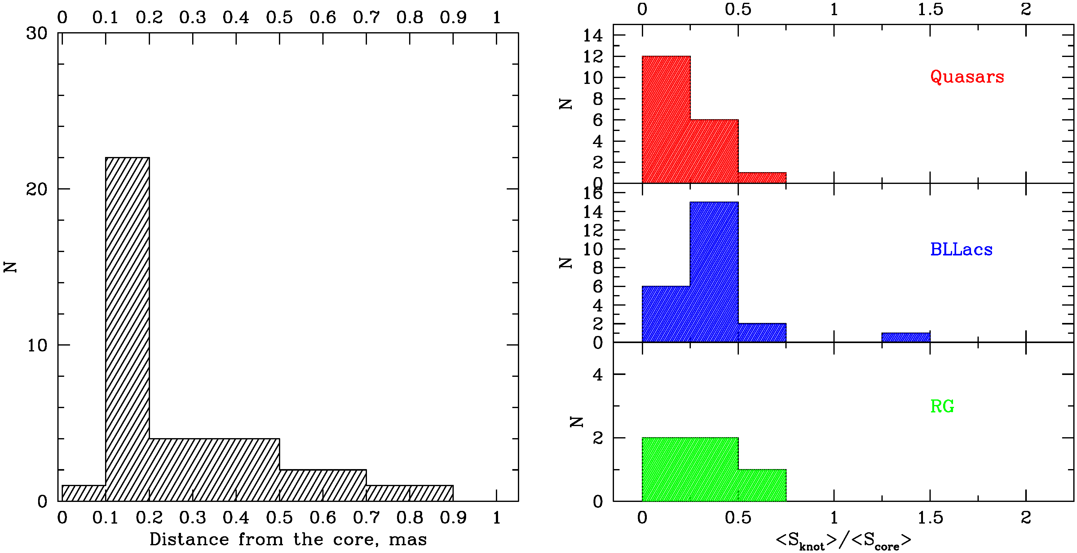Figure 1 (left) shows the distribution of distances of the stationary knots with respect to the core, which indicates that the most common location of stationary components is within 0.1–0.2 mas of the core. The latter agrees with the finding reported in [7], where observations have been performed at 43 and 22 GHz and stationary features near the core are detected at both frequencies. This supports the reality of such features rather than the option that they are artificial and caused, e.g., by gaps in uv-coverage. If the core at mm waves is a standing conical shock as suggested in [17], and the jet is sufficiently symmetric, numerical simulations predict the existence of several recollimation shocks in addition to the core [18], which can be responsible for stationary features observed near the core. We have calculated the average flux density of the core for each source in the sample and for each stationary feature. Figure 1 (right) plots the distributions of the averaged flux densities of stationary features normalized by the corresponding averaged flux density of the core for FSQs, BLLacs, and RGs. In general, 90% of stationary features are weaker than the core by a factor of ≥2. However, the peak of the distribution for BLLacs indicates that BL Lac objects are more likely to have brighter stationary features.

3.2. Superluminal and Subluminal Motion

Features classified as moving knots must be identified at ≥3 successive epochs and have a proper motion exceeding 2σ uncertainty in μ. The majority of moving knots propagate down the jet and are associated with flares in the core region. We assume that such knots were passing through the core during these flares. We extrapolate the motion of a knot back to the position of the core and calculate the time of the passage of the centroid of the knot through the centroid of the core, which we refer to as the ejection time, $T_{\circ }$. $T_{\circ }$ is the average of $t_{xo}$ and $t_{yo}$ weighted by their uncertainties, where $t_{xo}$ and $t_{yo}$ are the times when the position of the knot was at $x=0$ and $y=0$, respectively. Moving knots are designated as $Bn$, $Cn$, or $Dn$, with $T_{\circ }$ of $Cn$ and $Dn$ having occurred before the period of our monitoring and n corresponding to the number of the knot, ordered with respect to its distance from the core, with the most distant knot having $n=1$. Knots $Dn$ are the most diffuse features, with average size exceeding 0.5 mas. Among the $Bn$ and $Cn$ knots there is a special subclass of features that appear behind faster moving knots. Such knots are not seen at epochs at which they should be closer to the core according their kinematics, which implies that they are not ejected from the core. We classify these as trailing features, which form in jets behind a main perturbation [19]. We designate trailing components as $bn$ or $cn$, where n is the same number as for knot $Bn$ or $Cn$, respectively, behind which the trailing knot is detected. 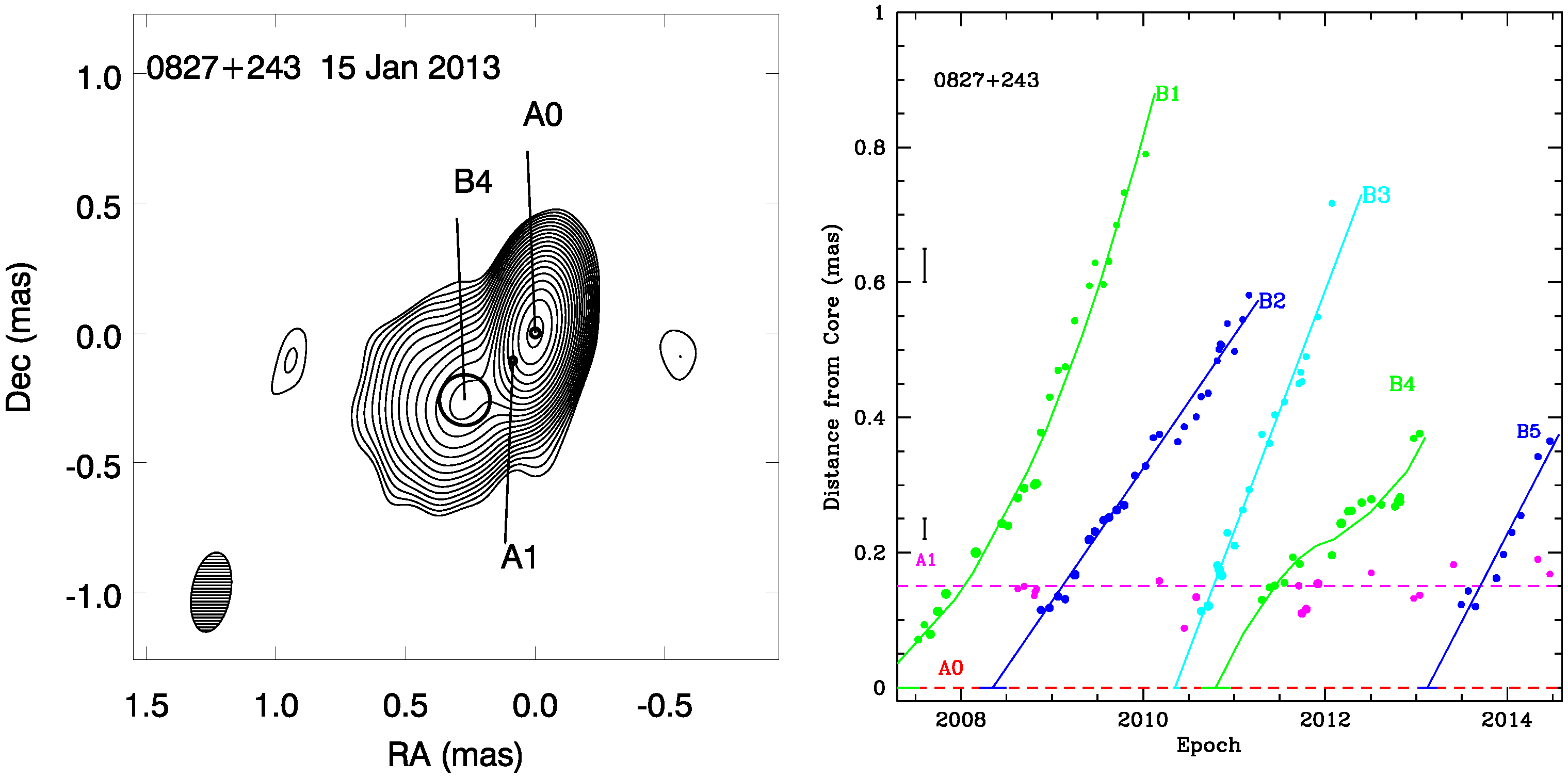Figure 2 (left) gives an example of an image of the quasar with knots detected at a given epoch indicated, while Figure 2 (right) presents the separation of knots from the core and approximation of the knot’s motion by polynomials of different orders.

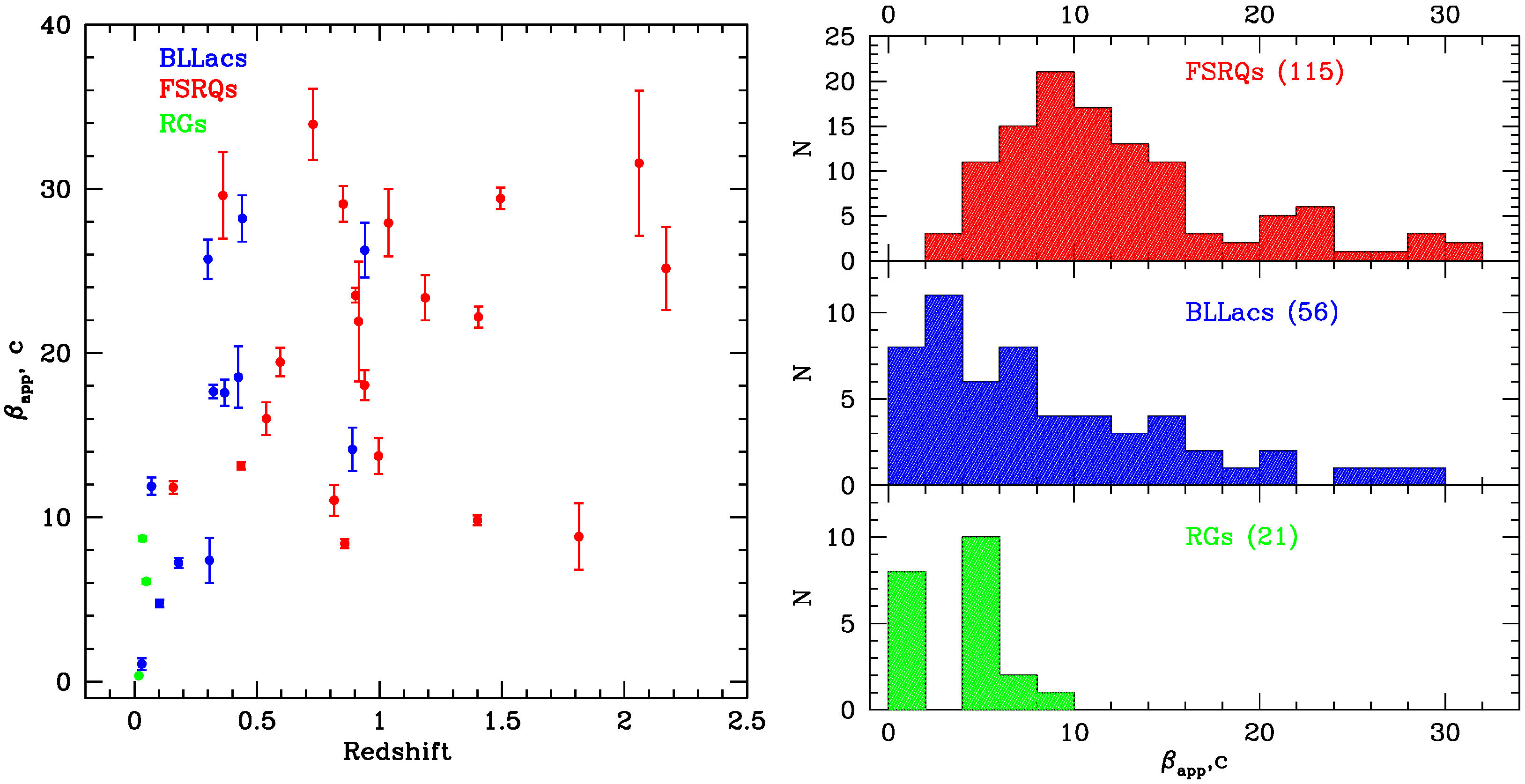
We have measured apparent speeds of 192 components (115 in FSRQs, 56 in BLLacs, and 21 in RGs). The apparent jet velocities are determimed for all sources in the sample. Out of 36 blazars, 34 possess knots with superluminal speeds, while the BL Lac object Mrk421 and the radio galaxy 3C84 have only jet features with subluminal speeds. Figure 3 (left) plots the maximum apparent speeds for each source vs. redshift, which shows that, for all quasars and the majority of BLLacs in the sample, ${\beta }_{app}^{max}\ge$ 10c. This implies that the Lorentz factor of the jets, Γ, exceeds 10. Figure 3 (right) displays the distributions of all moving knots for FSRQ, BLLacs, and RGs in the sample. It shows that the most common apparent speeds in jets of FSRQs and BLLacs are 8–10c and 2–4c, respectively. Note that 57% of BLLacs and 62% of FSRQs have speeds that fall within these respective ranges. If BLLacs possess $\mathsf{\Gamma }>10$, more common slower apparent speeds can be explained if the jets of BLLacs have larger viewing angles, ${\mathsf{\Theta }}_{\circ }$, and/or opening angles, ${\theta }_{\circ }$, than the jets of FSRQs. This should favor ejections when a disturbance has ${\mathsf{\Theta }}_{\circ }$ different from the value of $\sim 1/\mathsf{\Gamma }$, which maximizes the apparent speed of a knot with Lorentz factor Γ. Although this explanation is not unique, a hint of such dichotomy was found in [13] as well.

4. The Connection between Gamma-Ray and Radio Events

We have analyzed the γ-ray light curves of the sources in our sample to determine periods of γ-ray activity and γ-ray flares. We have calculated the weighted mean γ-ray fluxes, $\langle S_{\gamma }\rangle$, and their standard deviations, ${\sigma }_{\gamma }$, as described in [16], and determined active periods for each source when $S_{\gamma }>\langle S_{\gamma }\rangle +{\sigma }_{\gamma }$ over at least 2 successive measurements in the light curves with a binning interval of 7 days. We assume that 2 periods of activity are different if they are separated by >30 days. For each active period we have constructed a light curve with a 1 day binning interval, if $S_{\gamma }>1\times {10}^{-6}$ ph s${}^{-1}$ cm${}^{-2}$ in the initial light curve, and with a 3 day binning interval otherwise. We have searched these light curves for the brightest γ-ray outbursts with $S_{\gamma }>\langle S_{\gamma }\rangle +3{\sigma }_{\gamma }$ over at least 2 successive observations. Again, we consider 2 outbursts as different events if they are separated by >30 days, which is connected with the monthly cadence of the VLBA observations. We refer to such γ-ray outbursts as 3${\sigma }_{\gamma }$ flares. 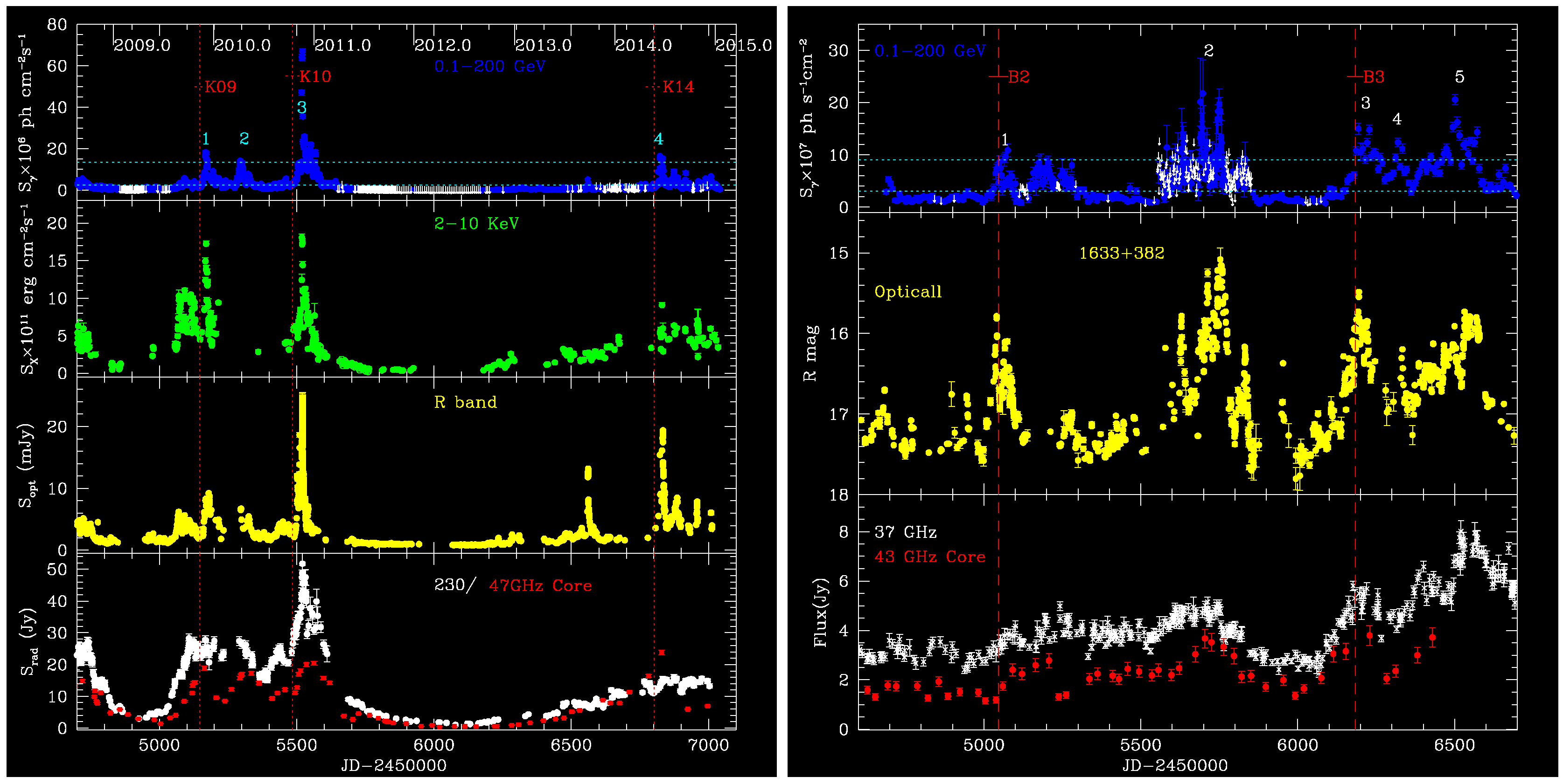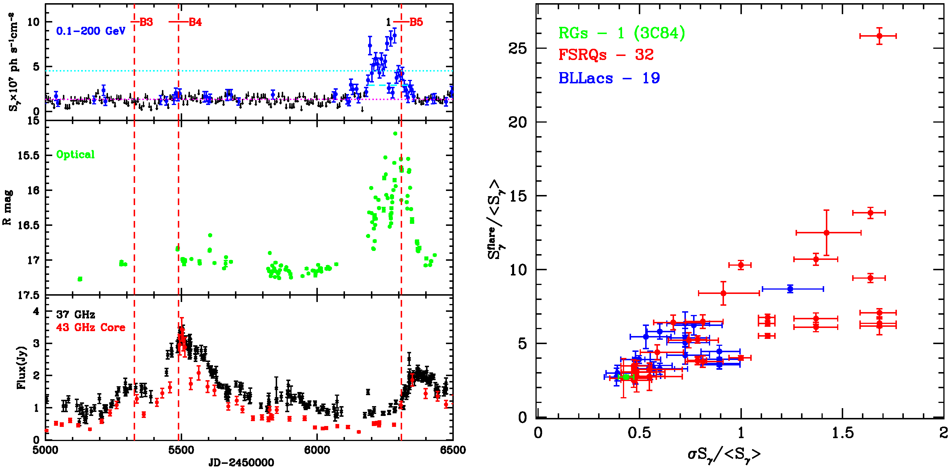Figure 4 (left) shows the γ-ray light curves of the quasar 0827+243 where one γ-ray event is classified as a 3${\sigma }_{\gamma }$ flare. The figure shows the optical and mm wave light curves of the quasar as well as times of ejection of superluminal knots, the kinematics of which is given in Figure 2 (right).

Overall, from August 2008 to January 2013, we detected 52 3${\sigma }_{\gamma }$ flares in our sample. Figure 4 (right) gives the general characteristics of γ-ray variability for these events, where $S_{\gamma }^{flare}$ is the maximum γ-ray flux during a flare. We determine the time of the peak of each flare $T_{\gamma }$ corresponding to $S_{\gamma }^{flare}$, and the duration of a 3${\sigma }_{\gamma }$ flare, $\mathrm{\Delta }{T}_{\gamma }$, as the time interval during which $S_{\gamma }>\langle S_{\gamma }\rangle +1.5{\sigma }_{\gamma }$.

We have calculated the average core flux, $\langle S_{core}\rangle$, and its standard deviation, ${\sigma }_{core}$, using core light curves derived from fluxes obtained from analysis of the VLBA data. Based on these parameters and results of the jet kinematics, we have searched for radio events of two types—core and ejection events. The core events are those when the VLBI core of a source has a 3${\sigma }_{core}$ flare defined in the same manner as a 3${\sigma }_{\gamma }$ flare. The time, $T_{core}$, and duration, $\mathrm{\Delta }{T}_{core}$ are determine similar to 3${\sigma }_{\gamma }$ flares as well. Ejection events require an ejection of a superluminal knot into the jet and the time of such an event is the time of the passage of a knot through the core, $T_{\circ }$, with duration corresponding to the 1σ uncertanty of the ejection time, $\pm \mathrm{\Delta }{T}_{\circ }$. Note that $\mathrm{\Delta }{T}_{\circ }$ describes the accuracy of measurements and does not take into account that the core and knot are not point sources. The latter can result in $T_{\circ }$ being a time interval, a complication that is not discussed here. Although core flares and ejection events are usually associated with each other [21], for some core flares ejection events are not apparent in our images. Figure 5 (left) shows light curves of the quasar 3C454.3 at different wavelengths with four 3${\sigma }_{\gamma }$ flares marked. All four flares have corresponding flares in the X-ray (no X-ray data for flare #2), optical, and mm wave light curves, and in the core, while only three of them (except #2) are associated with ejection events. Analysis of the multi-wavelength outburst #1–3 of 3C454.3 along with ejection events can be found in [22]. Figure 5 (right) shows γ-ray, optical, mm wave, and core light curves of the quasar 1633+382, which reveal similar behavior. Three 3${\sigma }_{\gamma }$ flares (#1–3) have contemporaneous optical and core flares, while for the most prominent γ-ray flare, #2, which is accompanied by a dramatic optical outburst, an ejection event is not seen in our images.

We compare 3${\sigma }_{\gamma }$ flares with core and ejection events. We associate a γ-ray flare with a core flare if $T_{\gamma }$ is within the core flare duration. We associate a γ-ray flare with an ejection event if $T_{\circ }-\mathrm{\Delta }{T}_{\circ }<T_{\gamma }<T_{\circ }+\mathrm{\Delta }{T}_{\circ }$. In general, we see core flares for all 3${\sigma }_{\gamma }$ flares identified, although for a few sources, these are not 3${\sigma }_{core}$ flares, rather 1-2${\sigma }_{core}$ events. The majority of the 3${\sigma }_{\gamma }$ flares (∼83%) are associated with ejection events and usually an ejection event leads the corresponding γ-ray flare.

The situation becomes more complicated when examining whether each ejection event has an accompanying γ-ray flare. Out of 171 moving features identified in FSRQs and BLLacs, 114 have ejection times within the period of our VLBA data analysis with Fermi LAT data available, from August 2008 to January 2014. During this period we have identified 52 3${\sigma }_{\gamma }$ flares, as mentioned above. This implies that more than 50% of ejection events are either not responsible for γ-ray flares or associated with milder γ-ray events than 3${\sigma }_{\gamma }$ flares. As is apparent in Figure 4 (left), two ejection events (knots B3 and B4) in the quasar 0827+243, associated with strong core flares, do not produce significant variations in the γ-ray emission, although during the $B4$ ejection the γ-ray flux changes from a non-detection to a detection (TS-statistic >10).

5. Summary

We are performing a comprehensive program of multi-wavelength monitoring of a sample of γ-ray blazars, the VLBA-BU-BLAZAR program. Here we have briefly presented the results on the parsec-scale jet kinemetics of the blazars from June 2007 to January 2013 and the connection between strong γ-ray flares and events in the radio jets. We summarize our preliminary results as follows:

(1)

Apparent speeds have been determined for 240 features in 21 FSRQs, 12 BLLacs, and 3 RGs, with 48 components classified as stationary features.

(2)

The majority of stationary features are located within 0.1–0.2 mas of the VLBI core.

(3)

For all sources in the sample, except two (3C84 and Mrk421), superluminal apparent speeds are measured for moving knots. The distribution of apparent speeds of the quasars peaks at 8–10c, while slower jet velocities are more common for the BLLacs, although the maximum apparent speeds in the jets are comparable for both sub-classes.

(4)

52 prominent γ-ray flares are identified in the sample from August 2008 to January 2013.

(5)

The γ-ray flares are contemporaneous with an increase of the flux in the 43 GHz VLBI core, which suggests that a disturbance propagating in the jet is necessary to produce a strong γ-ray event.

(6)

About 83% of the γ-ray flares occurred near the extrapolated time of the passage of superluminal knots through the VLBI core.

(7)

Approximately 65% of superluminal knots do not trigger prominent γ-ray events.

These results support the idea that the majority of strong γ-ray events originate close to the VLBI core seen on mm wave images, within the parsec-scale jet, although a more comprehensive analysis of the statistical significance of associations between parsec-scale jet events and γ-ray flares is in preparation.