This section introduces the Hubble distance, the dark energy density, the curvature, the matter density and the comoving distance (which is presented as the integral of the inverse of the Hubble function). In the absence of a general analytical formula for the comoving distance, we introduce the Padé approximation. As a consequence, we deduce an approximate solution for the transverse comoving distance, the luminosity distance and the distance modulus. The shift that the Padé approximation introduces in the relationship for the poles is discussed. The calibration of the Padé approximation for the distance modulus on two astronomical catalogs allows deducing the minimax polynomial approximation for the observed distance modulus for SNs of Type Ia.
2.1. The Padé Approximant
We use the same symbols as in [
9], where the Hubble distance
is defined as:
We then introduce the first parameter:
where
G is the Newtonian gravitational constant and
is the mass density at the present time. The second parameter is
:
where Λ is the cosmological constant; see [
10]. The two previous parameters are connected with the curvature
by:
The comoving distance,
, is:
where
is the `Hubble function’:
The above integral does not have an analytical formula, except for the case of
, but the Padé approximant (see
Appendix B) gives an approximate evaluation, and the indefinite integral is (B3), where the coefficients
and
can be found in
Appendix A. The approximate definite integral for (
5) is therefore:
The transverse comoving distance
is:
and the approximate transverse comoving distance
computed with the Padé approximant is:
An analytic expression for
can be obtained when:
:
This expression is useful for calibrating the numerical codes, which evaluate when .
The luminosity distance is:
which in the case of
becomes:
and the distance modulus when
is:
The Padé approximant luminosity distance when
is:
and the Padé approximant distance modulus,
, in its compact version, is:
and, as a consequence, the Padé approximant absolute magnitude,
, is:
The expanded version of the Padé approximant distance modulus is:
with:
The above procedure can also be applied when the argument of the integral (
5) is expanded about z = 0 in a Taylor series of order six. The resulting luminosity distance,
, is:
where:
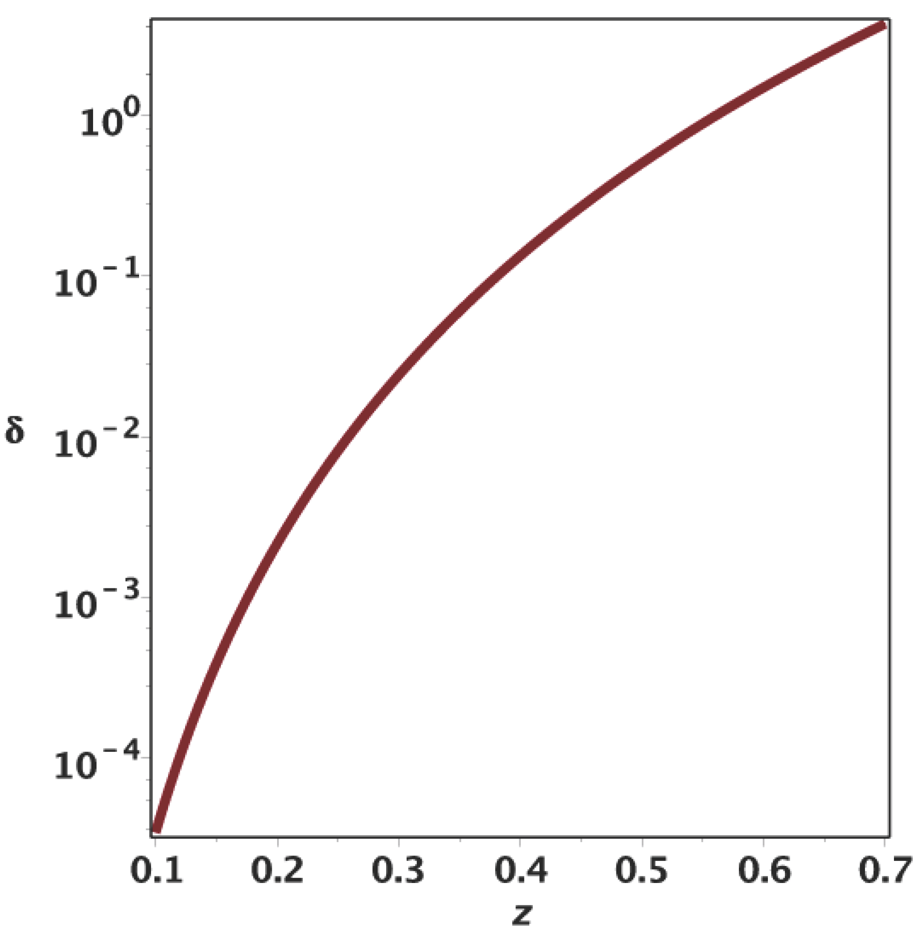
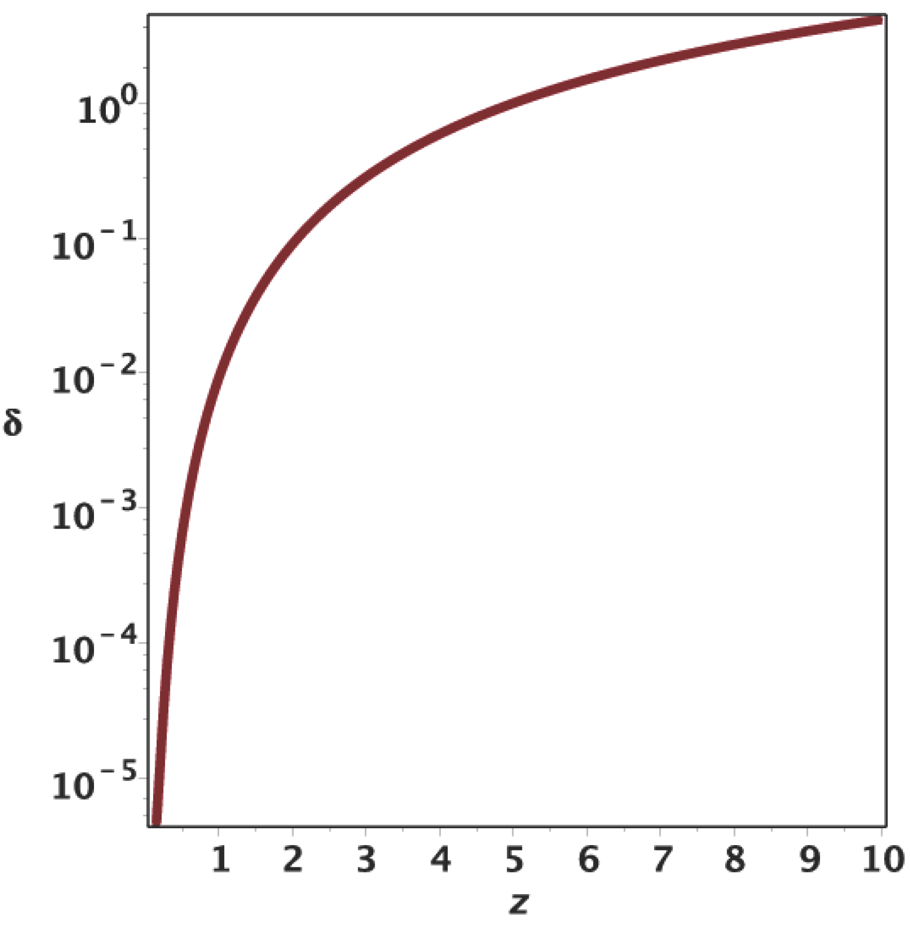
The goodness of the approximation is evaluated through the percentage error,
δ, which is:
where
is the exact luminosity distance when
(see Equation (
11)) and
is the Taylor or Padé approximate luminosity distance; see also Formula (2.12) in [
1].
Figure 1 and
Figure 2 report the percentage error as a function of the redshift
z for the Taylor and Padé approximations, respectively. The Padé approximation is superior to the truncated Taylor expansion, because
is reached at
for the Padé approximant and at
for the Taylor expansion.
2.3. An Astrophysical Application
We now have a Padé approximant expression for the distance modulus as a function of of
,
and
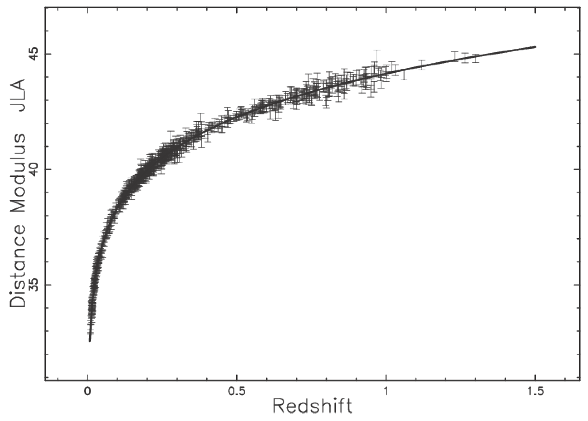
. We now perform an astronomical test on the 580 SNe in the Union 2.1 compilation (see [
5]) and on the 740 SNe in the joint light-curve analysis (JLA). The JLA compilation is available at the Strasbourg Astronomical Data Center (CDS) and consists of SNe (Type I-a) for which we have a heliocentric redshift,
z, apparent magnitude
in the B band, error in
,
, parameter
, error in
,
, parameter
C, error in the parameter
C,
and
. The observed distance modulus is defined by Equation (4) in [
6]:
The adopted parameters are
,
and:
see Line 1 in Table 10 of [
6]. The uncertainty in the observed distance modulus,
, is found by implementing the error propagation equation (often called the law of errors of Gauss) when the covariant terms are neglected; see Equation (3.14) in [
11],
The three astronomical parameters in question,
,
and
, can be derived trough the Levenberg–Marquardt method (subroutine MRQMINin [
12]) once an analytical expression for the derivatives of the distance modulus with respect to the unknown parameters is provided. As a practical example, the derivative of the distance modulus,
, with respect to
is:
This numerical procedure minimizes the merit function
evaluated as:
where
,
is the observed distance modulus evaluated at
,
is the error in the observed distance modulus evaluated at
and
is the theoretical distance modulus evaluated at
; see Formula (15.5.5) in [
12]. A reduced merit function
is evaluated by:
where
is the number of degrees of freedom,
n is the number of SNe and
k is the number of parameters. Another useful statistical parameter is the associated
Q-value, which has to be understood as the maximum probability of obtaining a better fitting; see Formula (15.2.12) in [
12]:
where GAMMQ is a subroutine for the incomplete gamma function. The Akaike information criterion (AIC) (see [
13]) is defined by:
where
L is the likelihood function. We assume a Gaussian distribution for the errors, and the likelihood function can be derived from the
statistic
, where
has been computed by Equation (
26); see [
14,
15]. Now, the AIC becomes:
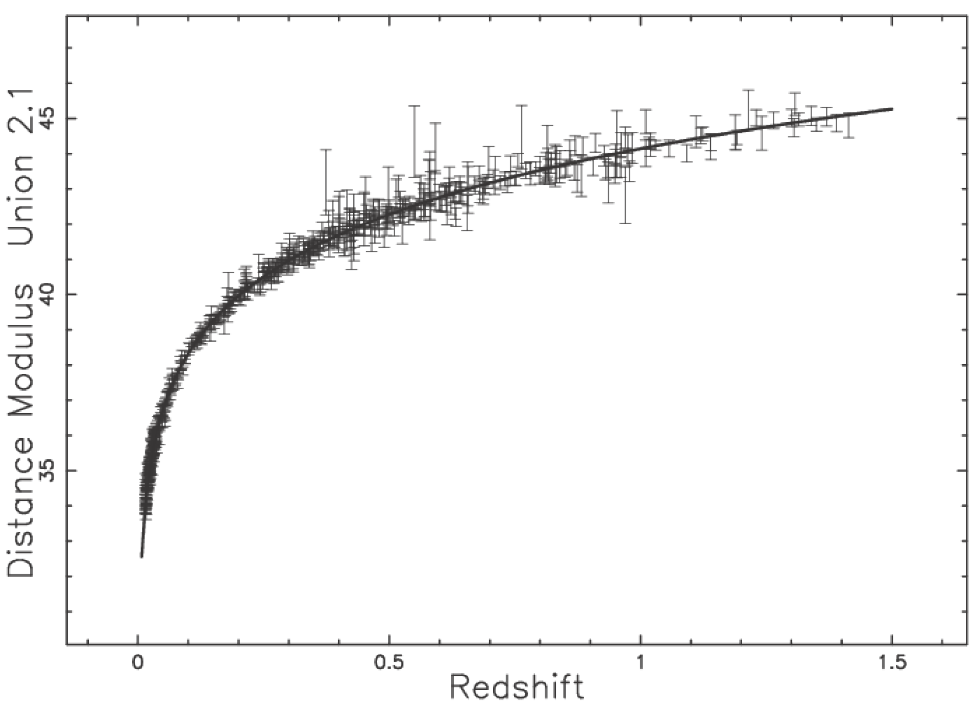
Table 1 reports the three astronomical parameters for the two catalogs of SNs, and
Figure 5 and
Figure 6 display the best fits.
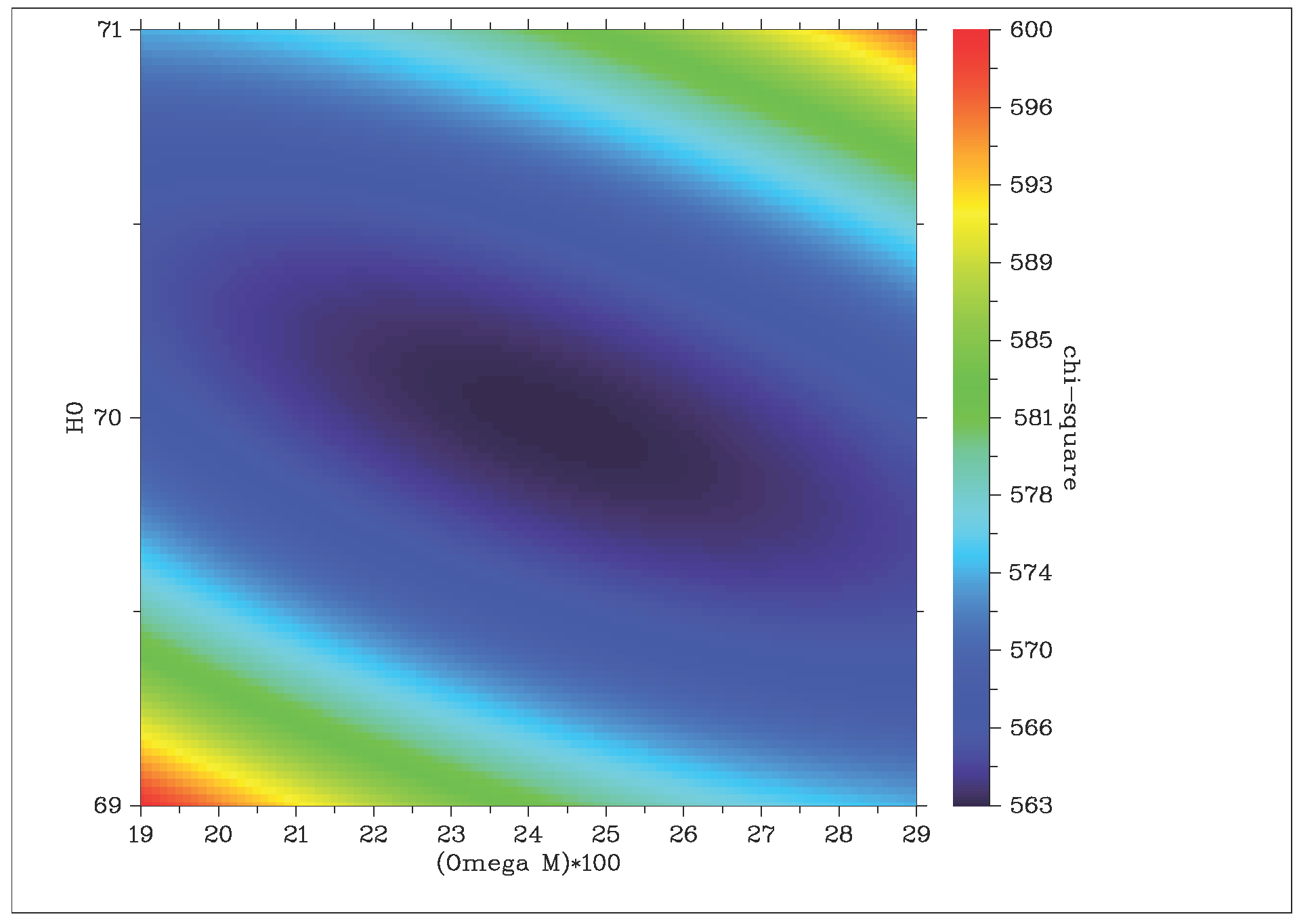
In order to see how
varies around the minimum found by the Levenberg–Marquardt method,
Figure 7 presents a 2D color map for the values of
when
and
are allowed to vary around the numerical values, which fix the minimum.
The Padé approximant distance modulus has a simple expression when the minimax rational approximation is used, as an example
; see
Appendix C for the meaning of
p and
q. In the case of the Union 2.1 compilation, the approximation of Formula (
17) with the parameters of
Table 1 over the range in
gives the following minimax equation:
the maximum error being 0.0024. The maximum error of the polynomial approximation as a function of
p and
q is shown in
Table 2.
In the case of the JLA compilation, the minimax equation is:
the maximum error being 0.003.
The maximum difference between the two minimax formulas, which approximate the distance modulus, Equations (
31) and (
32), is at
and is 0.0584 mag. In the case of the luminosity distance as given by the Padé approximation (see Equation (
14)), the minimax approximation gives:


