The I-Love Universal Relation for Polytropic Stars Under Newtonian Gravity

Abstract

The moment of inertia and tidal deformability of idealized stars with polytropic equations of state (EOSs) are numerically calculated under both Newtonian gravity and general relativity (GR). The results explicitly confirm that the relation between the moment of inertia and tidal deformability, parameterized by the star’s mass, exhibits variations up to $1\%$ and $10\%$ for different polytropic indices in Newtonian gravity and GR, respectively. This indicates a more robust I-Love universal relation in the Newtonian framework. The theoretically derived I-Love universal relation for polytropic stars is subsequently tested against observational data for the moment of inertia and tidal deformability of the eight planets and some moons in our solar system. The analysis reveals that the theoretical I-Love universal relation aligns well with the observational data, suggesting that it can serve as an empirical relation. Consequently, it enables the estimation of either the moment of inertia or the tidal deformability of an exoplanet if one of these quantities, along with the mass of the exoplanet, is known.

1. Introduction

The universal relations for neutron stars (NSs) and quark stars (QSs) were first identified by Yagi and Yunes in terms of the moment of inertia (I), tidal deformability (Love), and quadrupole moment (Q) of these compact stars [1,2]. These relations, known as I-Love-Q universal relations, are termed “universal” because they exhibit remarkable insensitivity to the equation of state (EOS) of the compact object. Even for EOSs that produce significantly different mass–radius relations for NSs and QSs, the I-Love-Q relations hold with a precision better than $1\%$. Subsequently, the universal relations were extended to include additional perturbative properties of compact stars, such as higher-order multipolar tidal deformabilities [3,4,5,6,7,8,9] and oscillation mode frequencies [10,11,12,13], and the univariate relations were generalized to bivariate relations [3,8,14,15,16]. In addition to the single star case, universal relations have also been found for binary neutron star mergers [17,18,19,20]. While these extended universal relations are valuable, their precision is generally lower than that of the original I-Love-Q relations, and in some cases, their discrepancies reach up to $10\%$ for different EOSs [9].

Though there are plausible arguments on why the universal relations exist [2,21], the precise mechanism underlying the universality of these relations remains unclear. Unlike the no-hair theorem for black holes in general relativity (GR) [22], the I-Love-Q universal relations are not exact and are established through numerical studies. Their accuracy often deteriorates when simplifying assumptions used in structural and perturbative calculations of stars are relaxed [23,24,25]. For instance, factors such as anisotropic pressure, non-barotropic EOSs, or the inclusion of more complex physics introduce greater discrepancies in the universal relations [26,27,28,29,30]. Moreover, the validity of the universal relations can also depend on the gravitational theory. While the I-Love universal relation has been shown to hold in many scalar-tensor theories (albeit with up to $10\%$ discrepancies) [31,32,33,34,35], it is visibly broken in specific scalar-tensor theories where the Gauss–Bonnet invariant is coupled to the square of a scalar field [36]. In such cases, the Schwarzschild solution is no longer unique, and scalarized black holes appear, violating the no-hair theorem [37,38,39]. Whether a connection exists between the breakdown of the I-Love universal relation and the violation of the no-hair theorem warrants further investigation.

Although the universal relations for NSs and QSs are widely studied because they mitigate EOS-related ambiguities in compact star studies, they are not exclusive to compact stars. As shown analytically in Ref. [2] using two specific polytropic EOSs, the I-Love-Q universal relations are also expected to apply to spherical objects in the Newtonian limit. Sham et al. in Ref. [40] further explained the I-Love-Q universal relations in the Newtonian limit by approximating the density inside a star as a constant plus a small correction quadratic in the distance to the center of the star; the approximation of the density profile enables them to explain the I-Love-Q universal relations in terms of the smallness of the correction analytically. Then, Yip and Leung in Ref. [41] investigated the I-Love universal relation in the Newtonian limit using an expansion method that generates the tidal Love number for any polytropic EOS with the polytropic index n in $[0,3]$ as expansion series around the two exactly solvable cases $n=0$ and $n=1$; they found two stationary points, $n=0$ and $n\approx 0.4444$, which explains the insentitivity of the I-Love relation to n.

Complementary to the insightful but dedicated analytical results in the literature on the I-Love universal relation in the Newtonian limit, we cut to the chase by providing plain and straightforward numerical calculations to update and summarize the results for readers looking for a quick knowledge on the subject. The tidal Love number and the moment of inertia for a polytropic star with general values of the polytropic index are numerically calculated in both Newtonian gravity and GR, using a unified framework of the perturbation theory. A comprehensive collection of diagrams plotted using representative numerical results are shown to illustrate properties, including the mass, the radius, the tidal Love number, the moment of inertia, and the compactness, of a polytropic star. The most important part of our work lies in the application of the I-Love universal relation to the solar-system planets and their moons. Despite their layered structures and complex compositions, which deviate from simple polytropic EOSs, these celestial objects conform well to the I-Love universal relation. This finding highlights the potential of the I-Love relation as a powerful tool not only for studying compact stars but also for deducing properties of exoplanets.

We begin by reviewing the formulae used to calculate the tidal deformability and the moment of inertia in Newtonian gravity in Section 2.1, and in general relativity (GR) in Section 2.2. In Section 2.3, we present numerical results for polytropic EOSs. In Section 2.4, we list and plot measurements of the tidal Love number and the moment of inertia for 17 planets and moons, comparing them with the I-Love universal relation for polytropic stars. A brief summary is provided in Section 3.

It is worth noting that the I-Love relation for white dwarfs deviates slightly from the I-Love universal relations in both Newtonian gravity and GR. The relevant results are included in Appendix A. Throughout this work, geometrized units are used, where the gravitational constant G and the speed of light c are set to 1. SI units are also employed to express the values of physical quantities. The metric sign convention used is $(-,+,+,+)$.

2. I-Love Universal Relations for Polytropic Stars

2.1. Newtonian Gravity

A comprehensive account of the spherically hydrostatic stars with polytropic EOSs and their perturbations can be found in Ref. [42]. We briefly review the formulae here. First, the basic set of equations consists of Poisson’s equation and the energy–momentum conservation equations:

$$\begin{array}{ccc}& & {\nabla }^2\Phi =-4\pi \rho ,\hfill \\ & & {\displaystyle \frac{\partial \rho }{\partial t}}+\nabla ·\left(\rho \mathit{v}\right)=0,\hfill \\ & & {\displaystyle \frac{\partial \mathit{v}}{\partial t}}+\left(\mathit{v}·\nabla \right)\mathit{v}=\nabla \Phi -{\displaystyle \frac{1}{\rho }}\nabla p,\hfill \end{array}$$

(1)

where $\Phi$ is the Newtonian potential, and $\rho ,p,\mathit{v}$ are the density, the pressure, and the velocity of the fluid constituting the star. Then, the variables assume the form

$$\begin{array}{ccc}& & \Phi ={\Phi }^{\left(0\right)}+\delta \Phi ,\hfill \\ & & \rho ={\rho }^{\left(0\right)}+\delta \rho ,\hfill \\ & & p=p^{\left(0\right)}+\delta p,\hfill \\ & & \mathit{v}={\mathit{v}}^{\left(0\right)}+\delta \mathit{v}.\hfill \end{array}$$

(2)

The zeroth-order terms correspond to the spherically symmetric hydrostatic solution, while the perturbation terms account for the tidal perturbation under consideration. If one assumes that the zeroth-order terms of the variables depend only on the radial coordinate r, with ${\mathit{v}}^{\left(0\right)}=0$, the hydrostatic equations for spherical Newtonian stars are obtained:

$$\begin{array}{ccc}& & {\Phi }^{\left(0\right)}″+{\displaystyle \frac{2}{r}}{\Phi }^{\left(0\right)}\prime =-4\pi \rho ,\hfill \\ & & p^{\left(0\right)}\prime ={\rho }^{\left(0\right)}{\Phi }^{\left(0\right)}\prime ,\hfill \end{array}$$

(3)

where the prime denotes the derivative with respect to r.

For the perturbation of Equation (1), it is convenient to use the Lagrangian displacement $\mathit{\xi }$ of the perturbed fluid elements. Without considering the uninteresting odd-parity perturbations, $\mathit{\xi }$ can be expressed in terms of the even-parity spherical harmonics,

$$\begin{array}{c}\hfill \mathit{\xi }=\left(\mathit{dr}{W}_1+\mathit{d}\mathit{\theta }V{\partial }_{\theta }+\mathit{d}\mathit{\varphi }V{\partial }_{\varphi }\right)Y_{lm},\end{array}$$

(4)

where $\{\mathit{dr},\mathit{d}\mathit{\theta },\mathit{d}\mathit{\varphi }\}$ is the basis for covariant components of vectors and tensors in the spherical coordinates $\left(r,\theta ,\varphi \right)$, $W_1$ and V are functions depending on r only, and $Y_{lm}$ refers to the usual spherical harmonics. We note that $\left(\mathit{d}\mathit{\theta }{\partial }_{\theta }+\mathit{d}\mathit{\varphi }{\partial }_{\varphi }\right)Y_{lm}$ comes from the even-parity vector spherical harmonics [43]

$$\begin{array}{ccc}\hfill {\mathit{Y}}_{lm}^E& :=& {\displaystyle \frac{r}{\sqrt{l(l+1)}}}\nabla Y_{lm}\hfill \\ & =& {\displaystyle \frac{r}{\sqrt{l(l+1)}}}\left(\mathit{d}\mathit{\theta }{\partial }_{\theta }+\mathit{d}\mathit{\varphi }{\partial }_{\varphi }\right)Y_{lm}.\hfill \end{array}$$

(5)

Using $\mathit{\xi }$, the perturbations of the density, the pressure, and the velocity are

$$\begin{array}{ccc}& & \delta \rho =-\rho \nabla ·\mathit{\xi }-\left(\mathit{\xi }·\nabla \right)\rho ,\hfill \\ & & \delta p=-{\Gamma }_{1}p\nabla ·\mathit{\xi }-\left(\mathit{\xi }·\nabla \right)p,\hfill \\ & & \delta \mathit{v}={\partial }_t\mathit{\xi }+\left(\mathit{v}·\nabla \right)\mathit{\xi }-\left(\mathit{\xi }·\nabla \right)\mathit{v},\hfill \end{array}$$

(6)

where ${\Gamma }_1$ is the adiabatic index for fluid elements under the perturbations. For barotropic EOSs where p depends solely on $\rho$, one has

$$\begin{array}{c}\hfill {\Gamma }_1={\displaystyle \frac{\rho }{p}}{\displaystyle \frac{dp}{d\rho }}.\end{array}$$

(7)

Especially, for the polytropic EOSs

$$\begin{array}{c}\hfill p=\alpha {\rho }^{1+\frac{1}{n}},\end{array}$$

(8)

where $\alpha$ and n are constants, we have ${\Gamma }_1=1+1/n$, with n being the polytropic index.

To simplify the calculation of the tidal Love number, we assume the fluid to be incompressible, namely

$$\begin{array}{c}\hfill \nabla ·\mathit{v}=0.\end{array}$$

(9)

It indicates that $d\rho /dt=0$ when combined with the mass conservation equation in Equation (1). So, it is valid when the density of the fluid element stays unchanged along its trajectory. Using Equations (4) and (6) to write out the linear order of Equation (9) and the Euler equation in Equation (1), one finds that the variables $W_1$ and V can be expressed in terms of $\delta \Phi$ and $\delta {\Phi }^{\prime }$:

$$\begin{array}{ccc}& & W_1=-{\displaystyle \frac{\rho }{p^{\prime }}}\delta \Phi ,\hfill \\ & & V={\displaystyle \frac{r^2}{l(l+1)}}{W}_1^{\prime }-{\displaystyle \frac{2r\rho }{l(l+1)p^{\prime }}}\delta \Phi .\hfill \end{array}$$

(10)

Poisson’s equation in Equation (1) then gives an ordinary differential equation (ODE) for $\delta \Phi$:

$$\begin{array}{c}\hfill \delta \Phi ″+{\displaystyle \frac{2}{r}}\delta {\Phi }^{\prime }+\left(4\pi \rho {\displaystyle \frac{{\rho }^{\prime }}{p^{\prime }}}-{\displaystyle \frac{l(l+1)}{r^2}}\right)\delta \Phi =0.\end{array}$$

(11)

Equations (10) and (11) are supposed to be valid at the linear order, so $\rho ,p$ and their radial derivatives take the zeroth-order values. Equation (11) has the simple solution $C_l{r}^l+D_l{r}^{-l-1}$ outside the star, where $C_l$ and $D_l$ are constants. Interpreting the $r^l$ terms as an external tidal field and the $r^{-l-1}$ terms as the multipolar response of the star to the external tidal field, the tidal Love numbers are defined as

$$\begin{array}{c}\hfill k_l:={\displaystyle \frac{1}{2}}{\displaystyle \frac{1}{R^{2l+1}}}{\displaystyle \frac{D_l}{C_l}},\end{array}$$

(12)

where R is the radius of the star. Focusing on the lowest tidal term that is proportional to $r^2$, it causes a quadrupole term as the response, namely that it is the $l=2$ case. In this case, the tidal deformability is defined as

$$\begin{array}{c}\hfill {\lambda }_2:={\displaystyle \frac{1}{3}}{\displaystyle \frac{D_2}{C_2}}={\displaystyle \frac{2k_2}{3}}{R}^5.\end{array}$$

(13)

The fluid variables and the Newtonian potential need to be finite at the center of the star. This turns out to be a condition that fixes the ratios between $C_l$ and $D_l$, so that $k_l$ can be calculated uniquely given a solution of $\delta \Phi$ inside the star. In fact, an expansion analysis of Equations (3) and (11) leads to

$$\begin{array}{ccc}& & {\Phi }^{\left(0\right)}\prime \approx -{\displaystyle \frac{4\pi }{3}}r{\rho }_0,\hfill \\ & & p^{\left(0\right)}\approx p_0,\hfill \\ & & \delta \Phi \approx A_l{r}^l,\hfill \end{array}$$

(14)

at $r\to 0$, where ${\rho }_0$ and $p_0$ are the density and the pressure at the center of the star, and $A_l$ represents constants that simply scale the solution of $\delta \Phi$. For a given EOS, ${\rho }_0$ and $p_0$ are related. Therefore, the solutions to Equations (3) and (11) are controlled by one free parameter.

Given a barotropic EOS, one can numerically integrate Equations (3) and (11) from a tiny r where the approximation in Equation (14) is valid to a radius where p vanishes to obtain the solution inside the star. By matching $\delta \Phi$ and $\delta {\Phi }^{\prime }$ at the surface of the star to the exterior solution $C_l{r}^l+D_l{r}^{-l-1}$, $C_l$ and $D_l$ can be determined so that $k_l$ can be calculated. As for the moment of inertia, it is obtained simply through the integral

$$\begin{array}{c}\hfill I=\int {\left(rsin\theta \right)}^2{\rho }^{\left(0\right)}{d}^{3}x.\end{array}$$

(15)

2.2. General Relativity

The perturbation theory in GR to calculate the moment of inertia and the tidal deformability of a static spherical star is well-established in the literature; e.g., see Refs. [44,45,46,47]. To compare with the formulae in Newtonian gravity parallelly, we briefly review the GR counterpart.

The basic equations to start with are the Einstein field equations

$$\begin{array}{c}\hfill G_{\mu \nu }=8\pi T_{\mu \nu },\end{array}$$

(16)

with the energy–momentum tensor of the fluid

$$\begin{array}{c}\hfill T_{\mu \nu }=\left(ϵ+p\right)u_{\mu }{u}_{\nu }+p{g}_{\mu \nu },\end{array}$$

(17)

where $ϵ,p$, and $u_{\mu }$ are the proper energy density, the proper pressure, and the four-velocity of the fluid elements. The energy–momentum conservation equation $D^{\mu }{T}_{\mu \nu }=0$, where $D_{\mu }$ is the covariant derivative, is a consequence of the Einstein field equations. The variables are set up to be the static spherical background configuration plus perturbations, namely

$$\begin{array}{ccc}& & g_{\mu \nu }=g_{\mu \nu }^{\left(0\right)}+\delta g_{\mu \nu },\hfill \\ & & ϵ={ϵ}^{\left(0\right)}+\delta ϵ,\hfill \\ & & p=p^{\left(0\right)}+\delta p,\hfill \\ & & u_{\mu }=u_{\mu }^{\left(0\right)}+\delta u_{\mu }.\hfill \end{array}$$

(18)

Using the spherical ansatz

$$\begin{array}{c}\hfill g_{\mu \nu }^{\left(0\right)}d{x}^{\mu }d{x}^{\nu }=g_{tt}^{\left(0\right)}d{t}^2+{\left(1-{\displaystyle \frac{2m}{r}}\right)}^{-1}d{r}^2+r^{2}d{\Omega }^2,\end{array}$$

(19)

for the background metric, one obtains from the Einstein field equations the Tolman–Oppenheimer–Volkoff (TOV) equation

$$\begin{array}{ccc}& & m\prime =4\pi r^2{ϵ}^{\left(0\right)},\hfill \\ & & p^{\left(0\right)}\prime =-\left({ϵ}^{\left(0\right)}+p^{\left(0\right)}\right){\displaystyle \frac{m+4\pi r^3{p}^{\left(0\right)}}{r(r-2m)}},\hfill \end{array}$$

(20)

where the prime denotes the derivative with respect to r.

The perturbations are decomposed into spherical harmonic modes to naturally satisfy the angular dependence in the Einstein field equations. In addition to the even-parity vector spherical harmonics in Equation (5), we also need the odd-parity vector spherical harmonics [43]:

$$\begin{array}{ccc}\hfill {\mathit{Y}}_{lm}^B& :=& {\displaystyle \frac{1}{\sqrt{l(l+1)}}}\mathit{r}\times \nabla Y_{lm}\hfill \\ & =& {\displaystyle \frac{r}{\sqrt{l(l+1)}}}\left(-{\displaystyle \frac{\mathit{d}\mathit{\theta }}{sin\theta }}{\partial }_{\varphi }+\mathit{d}\mathit{\varphi }sin\theta {\partial }_{\theta }\right)Y_{lm}.\hfill \end{array}$$

(21)

In the Regge–Wheeler gauge [48], the even-parity perturbations of the metric are

$$\begin{array}{c}\hfill \delta g_{\mu \nu }=e^{i\sigma t}\left(\begin{array}{cccc}-g_{tt}^{\left(0\right)}{H}_0& H_1& 0& 0\\ \mathrm{sym}& g_{rr}^{\left(0\right)}{H}_2& 0& 0\\ 0& 0& r^{2}K& 0\\ 0& 0& 0& r^2{sin}^2\theta K\end{array}\right)Y_{lm},\end{array}$$

(22)

while the odd-parity perturbations of the metric are

$$\begin{array}{c}\hfill \delta g_{\mu \nu }=e^{i\sigma t}\left(\begin{array}{cccc}0& 0& -h_0{\displaystyle \frac{1}{sin\theta }}{\partial }_{\varphi }& h_{0}sin\theta {\partial }_{\theta }\\ 0& 0& -h_1{\displaystyle \frac{1}{sin\theta }}{\partial }_{\varphi }& h_{1}sin\theta {\partial }_{\theta }\\ \mathrm{sym}& \mathrm{sym}& 0& 0\\ \mathrm{sym}& \mathrm{sym}& 0& 0\end{array}\right)Y_{lm},\end{array}$$

(23)

where $H_0,H_1,H_2,K$, and $h_0,h_1$ are functions of r, and $\sigma$ is the oscillation frequency of the mode. The perturbations corresponding to a static tidal field and a slowly rigid rotation are time-independent, so the limit $\sigma \to 0$ is taken once the equations for the perturbation variables are obtained. The symbol “sym” means the symmetric property $\delta g_{\mu \nu }=\delta g_{\nu \mu }$.

For the perturbations in the fluid sector, the fundamental variable is the Lagrangian displacement ${\xi }_{\mu }$ for the perturbed fluid elements. It takes the form

$$\begin{array}{c}\hfill {\xi }_{\mu }=e^{i\sigma t}\left(W_0,W_1,V{\partial }_{\theta },V{\partial }_{\varphi }\right)Y_{lm},\end{array}$$

(24)

for the even parity, and

$$\begin{array}{c}\hfill {\xi }_{\mu }=e^{i\sigma t}\left(0,0,-U{\displaystyle \frac{1}{sin\theta }}{\partial }_{\varphi },Usin\theta {\partial }_{\theta }\right)Y_{lm},\end{array}$$

(25)

for the odd parity, where $W_0,W_1,V$, and U are functions of r. The perturbations of the energy density, the pressure, and the four-velocity can be expressed in terms of $\delta g_{\mu \nu }$ and ${\xi }_{\mu }$ via the following [49]:

$$\begin{array}{ccc}& & \Delta ϵ=-{\displaystyle \frac{1}{2}}(ϵ+p)\left(g^{\mu \nu }+u^{\mu }{u}^{\nu }\right)\Delta g_{\mu \nu },\hfill \\ & & \Delta p=-{\displaystyle \frac{1}{2}}{\Gamma }_{1}p\left(g^{\mu \nu }+u^{\mu }{u}^{\nu }\right)\Delta g_{\mu \nu },\hfill \\ & & \Delta u^{\mu }={\displaystyle \frac{1}{2}}{u}^{\mu }{u}^{\alpha }{u}^{\beta }\Delta g_{\alpha \beta }.\hfill \end{array}$$

(26)

We note that those are Lagrangian perturbations. The Eulerian perturbations that are directly used in the Einstein field equations can be obtained via $\Delta =\delta +{\mathcal{L}}_{\xi }$, where ${\mathcal{L}}_{\xi }$ is the Lie derivative along the vector ${\xi }_{\mu }$. For example,

$$\begin{array}{c}\hfill {\mathcal{L}}_{\xi }{u}^{\mu }={\xi }^{\alpha }{D}_{\alpha }{u}^{\mu }-u^{\alpha }{D}_{\alpha }{\xi }^{\mu }.\end{array}$$

(27)

In Equation (26), we use

$$\begin{array}{c}\hfill {\Gamma }_1={\displaystyle \frac{ϵ+p}{p}}{\displaystyle \frac{dp}{dϵ}},\end{array}$$

(28)

which is the relativistic version of the adiabatic index for fluid elements under the perturbations. We take

$$\begin{array}{c}\hfill p=\alpha {ϵ}^{1+\frac{1}{n}}\end{array}$$

(29)

as the relativistic version of the polytropic EOSs, so ${\Gamma }_1=(1+p/ϵ)(1+1/n)$ in this case. As $ϵ\approx \rho$ in the Newtonian limit, Equation (29) goes to Equation (8).

Substituting the perturbations of the metric and the perturbations in the fluid sector into the Einstein field equations and the energy–momentum conservation equation, one obtains ODEs for the variables $H_0,H_1,H_2,K,h_0,h_1$, and $W_1,V,U$. The variable $W_0$ disappears due to the static spherical background metric. We focus on the time-independent case to calculate the tidal deformability with the $l=2$ even-parity perturbation and the moment of inertia with the $l=1$ odd-parity perturbation.

With $\sigma =0$, the even-parity perturbation equations can be simplified to a single second-order ODE for $H_0$:

$$\begin{array}{ccc}& & H_0^{″}+{\displaystyle \frac{2(r-m)-4\pi r^3(ϵ-p)}{r\left(r-2m\right)}}{H}_0^{\prime }-{\displaystyle \frac{l(l+1)m}{r(r-2m)\left(m+4\pi r^{3}p\right)}}{H}_0-{\displaystyle \frac{4m^3}{r^2{(r-2m)}^2\left(m+4\pi r^{3}p\right)}}{H}_0\hfill \\ & & -{\displaystyle \frac{4\pi r^3\left(r{ϵ}^{\prime }+l(l+1)p+64{\pi }^2{r}^4{p}^3-20\pi r^2ϵp-36\pi r^2{p}^2\right)}{{(r-2m)}^2\left(m+4\pi r^{3}p\right)}}{H}_0\hfill \\ & & -{\displaystyle \frac{4\pi r^{2}m\left(40\pi r^2ϵp+120\pi r^2{p}^2-5ϵ-\left(2l^2+2l+9\right)p-4r{ϵ}^{\prime }\right)+8\pi r{m}^2\left(2r{ϵ}^{\prime }+5ϵ+15p\right)}{{(r-2m)}^2\left(m+4\pi r^{3}p\right)}}{H}_0=0.\hfill \end{array}$$

(30)

The physical solution behaves as

$$\begin{array}{c}\hfill H_0\approx A_l{r}^l,\end{array}$$

(31)

at the center of the star, and

$$\begin{array}{c}\hfill H_0\approx C_l{r}^l+D_l{r}^{-l-1},\end{array}$$

(32)

at infinity. By numerically solving Equation (30) from the center of the star to a large-enough radius, one can extract $C_l$ and $D_l$ from the solution, and hence calculate the tidal Love numbers using the same definition as in Equation (12) and the tidal deformability using the same definition as in Equation (13).

The odd-parity perturbation equations are much simpler than the even ones. In fact, the equation for the fluid variable U is algebraic. For the time-independent case, we have

$$\begin{array}{c}\hfill U\to {\displaystyle \frac{i}{\sigma }}\sqrt{{\displaystyle \frac{4\pi }{3}}}\tilde{\Omega }{r}^2,\end{array}$$

(33)

where $\tilde{\Omega }$ is a constant at the limit $\sigma \to 0$, so that the angular velocity of the star is

$$\begin{array}{c}\hfill \Omega =\sqrt{{\displaystyle \frac{2l+1}{3}}}\tilde{\Omega }{\displaystyle \frac{d}{dcos\theta }}{P}_l(cos\theta ).\end{array}$$

(34)

The rotation of the star is rigid for $l=1$ and differential for $l\ge 2$. The equation for $h_0$ in the time-independent case is

$$\begin{array}{ccc}& & h_0^{″}-{\displaystyle \frac{8\pi r^2(ϵ+p)}{2(r-2m)}}{h}_0^{\prime }-{\displaystyle \frac{8\pi r^3(ϵ+p)+l\left(l+1\right)r-4m}{r^2(r-2m)}}{h}_0\hfill \\ & & +{\displaystyle \frac{\sqrt{\frac{\pi }{3}}32\pi r^3(ϵ+p)}{r-2m}}\tilde{\Omega }=0.\hfill \end{array}$$

(35)

At the center of the star, the physical solution behaves as

$$\begin{array}{c}\hfill h_0\approx a_l{r}^{l+1}+h_{0\mathrm{in}},\end{array}$$

(36)

where $a_l$ are constants, and $h_{0\mathrm{in}}$ is a particular solution to Equation (35) and proportional to the constant $\tilde{\Omega }$. At infinity, the physical solution behaves as

$$\begin{array}{c}\hfill h_0\approx d_l{r}^{-l},\end{array}$$

(37)

where $d_l$ represents constants. Numerical integrations start near $r=0$, where Equation (36) is valid. By setting $a_l=1$ and adjusting $\tilde{\Omega }$ to a suitable value, the asymptotic behavior in Equation (37) can be achieved. Especially, for $l=1$, the asymptotic behavior in Equation (37) means that the metric component $g_{t\varphi }$ behaves as

$$\begin{array}{c}\hfill g_{t\varphi }\approx -{\displaystyle \frac{2J}{r}}{sin}^2\theta ,\end{array}$$

(38)

at infinity, where $J=\sqrt{3}{d}_1/\sqrt{16\pi }$ is the angular momentum of the spacetime. Therefore, the moment of inertia can be calculated via

$$\begin{array}{c}\hfill I={\displaystyle \frac{J}{\tilde{\Omega }}}=\sqrt{{\displaystyle \frac{3}{16\pi }}}{\displaystyle \frac{d_1}{\tilde{\Omega }}},\end{array}$$

(39)

once $d_1$ and $\tilde{\Omega }$ are known.

In practice, there is a trick to solve Equation (35) for $l=1$ only. A change of variable

$$\begin{array}{c}\hfill h_0=-\sqrt{{\displaystyle \frac{4\pi }{3}}}{r}^2(\omega -\tilde{\Omega }),\end{array}$$

(40)

simplifies Equation (35) to a homogeneous equation of $\omega$ for $l=1$. And outside the star, $\omega$ has the simple solution

$$\begin{array}{c}\hfill \omega =c+{\displaystyle \frac{d}{r^3}},\end{array}$$

(41)

where c and d are constants. For $h_0$ and $g_{t\varphi }$ to have the correct asymptotic behavior, one finds

$$\begin{array}{ccc}& & c=\tilde{\Omega },\hfill \\ & & d=-2J.\hfill \end{array}$$

(42)

Therefore, by numerically solving $\omega$ inside the star and matching $\omega$ and ${\omega }^{\prime }$ at the surface of the star, one obtains c and d, and hence $I=-d/\left(2c\right)$.

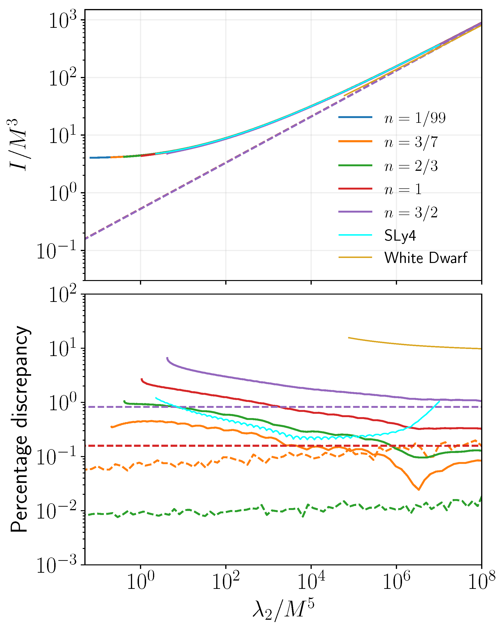
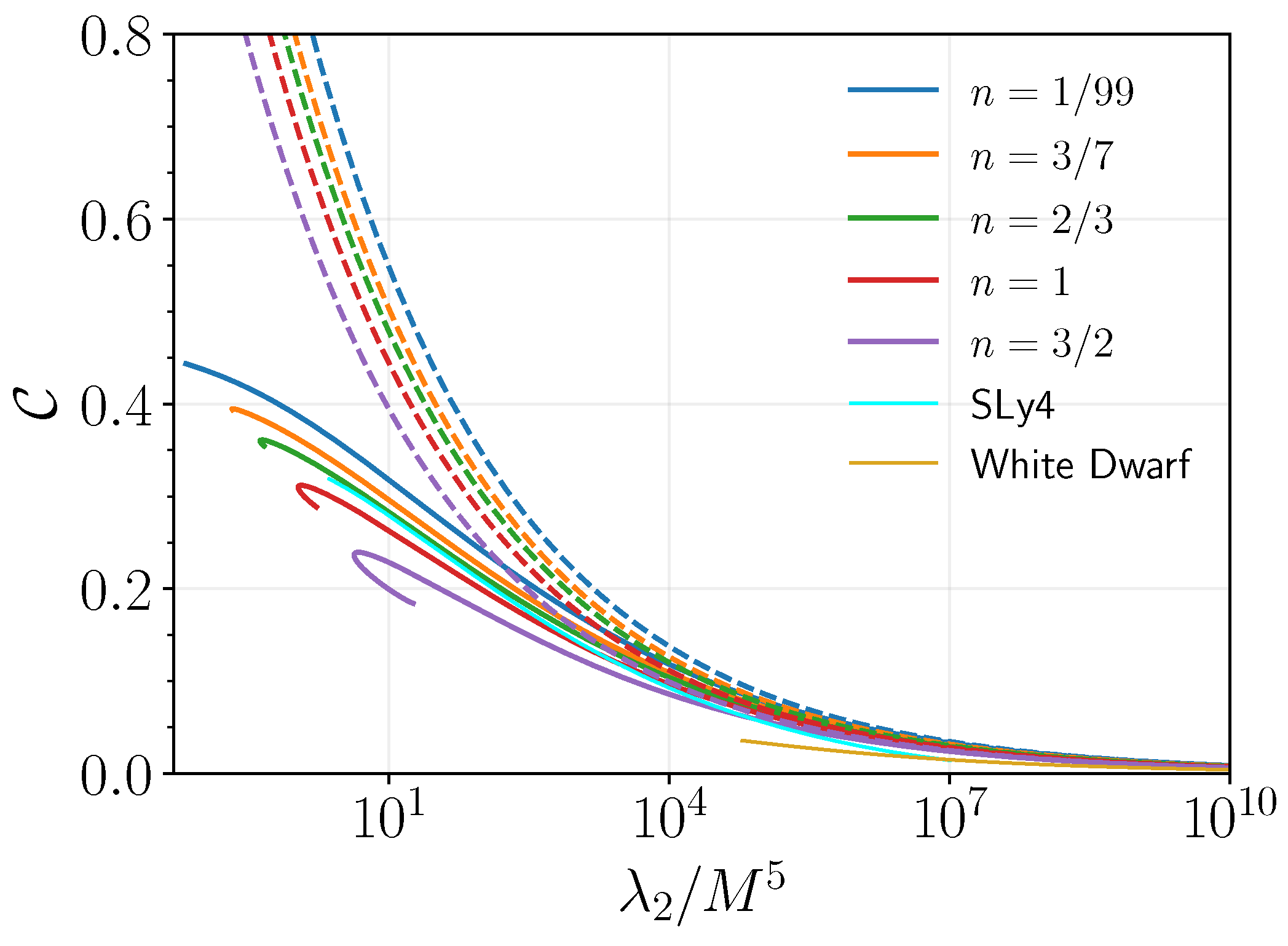
2.3. Numerical Results

Using the above formulae, we calculate the $l=2$ tidal deformability and the moment of inertia for polytropic stars in both Newtonian gravity and GR.

First, as a preparation for calculating the tidal deformability and the moment of inertia, masses and radii of the background spherical stars are calculated using polytropic EOSs with different values of indices. Figure 1 presents the results. The following length parameter is used as the unit of the mass and radius of the polytropic stars:

$$\begin{array}{c}\hfill L_{\mathrm{unit}}={\displaystyle \frac{1}{\sqrt{4\pi }}}{\alpha }^{n/2},\end{array}$$

(43)

where $\alpha$ is the dimensional coefficient, and n is the polytropic index in Equation (8) for Newtonian gravity and Equation (29) for GR.

One observation from Figure 1 merits addressing: the Newtonian mass–radius relations extend indefinitely as the central density and pressure approach infinity, meaning there is no maximal mass for Newtonian stars with polytropic EOSs, while the mass–radius relations in GR have maximal masses that mark critical points where the solutions start to be unstable.

Then, in Figure 2, results of the moment of inertia and the tidal deformability are converted to the moment of inertia factor $I/\left(M{R}^2\right)$ and the tidal Love number $k_2$, and plotted against the mass of the star. We point out that for a given polytropic index n, the moment of inertia factor $I/\left(M{R}^2\right)$ and the tidal Love number $k_2$ remain constant as the mass of the Newtonian star varies. This is due to a rescaling symmetry of the Newtonian problem.1

Finally, in Figure 3, the moment of inertia I and the tidal deformability ${\lambda }_2$, both parameterized by the mass of the star, are plotted. It is evident that different polytropic indices result in universal relations between $I/M^3$ and ${\lambda }_2/M^5$ in Newtonian gravity and GR separately. While the universal relation in Newtonian gravity meets the universal relation in GR at the higher end of ${\lambda }_2/M^5$, which is the regime of the Newtonian limit, they deviate from each other at the lower end of ${\lambda }_2/M^5$, corresponding to large masses and compact stars. The deviations between results for different values of n are smaller in Newtonian gravity than in GR, indicating that the universality of the relation holds more robustly in Newtonian gravity.

To assess the applicability of the polytropic EOS results to real stars, we also calculated ${\lambda }_2$ and I for NSs using the tabulated EOS SLy4 [50,51] and for white dwarfs using the theoretical EOS under the zero-temperature approximation (see Appendix A). For NSs, the $I/M^3$ versus ${\lambda }_2/M^5$ relation derived from EOS SLy4 aligns well with the universal relation for polytropic EOSs. For white dwarfs, there is a discrepancy of about $10\%$ between their $I/M^3$-versus-${\lambda }_2/M^5$ relation and the universal relation in GR. Notably, ${\lambda }_2$ and I for white dwarfs were calculated within the GR framework, so their $I/M^3$-versus-${\lambda }_2/M^5$ relation is compared with the universal relation in GR, even though Figure 3 shows that the line for white dwarfs is closer to the Newtonian line.

We note the analytical form of the universal relation in Newtonian gravity, obtained from the special case $n\to 0$. When $n\to 0$, the polytropic EOS describes stars with a uniform density, allowing for analytical solutions for Equations (3) and (11). Considering the density discontinuity at the star’s surface, one finds $k_2=3/4$ [42]. Additionally, $I/\left(M{R}^2\right)=2/5$ is known for a spherical star with a uniform density. Therefore, in this case, we obtain [52,53]

$$\begin{array}{c}\hfill {\displaystyle \frac{I}{M^3}}={\displaystyle \frac{2^{7/5}}{5}}{\left({\displaystyle \frac{{\lambda }_2}{M^5}}\right)}^{2/5}.\end{array}$$

(44)

Let us address the fact that the I-Love universal relation is completely nontrivial before we turn to its application. For demonstration, we plot in Figure 4 $I/R^3$ versus ${\lambda }_2/R^5$, where I and ${\lambda }_2$ are parameterized using the radius R rather than the mass M, and in Figure 5 the compactness $\mathcal{C}:=M/R$ versus ${\lambda }_2/M^5$. Neither of them is universal. The miraculous I-Love universal relation holds between I and ${\lambda }_2$, specifically parameterized by the mass of the star, not between any other seemingly plausible quantities. Note that the relation between the compactness and ${\lambda }_2/M^5$ is known to be nearly universal for NSs [17,54].

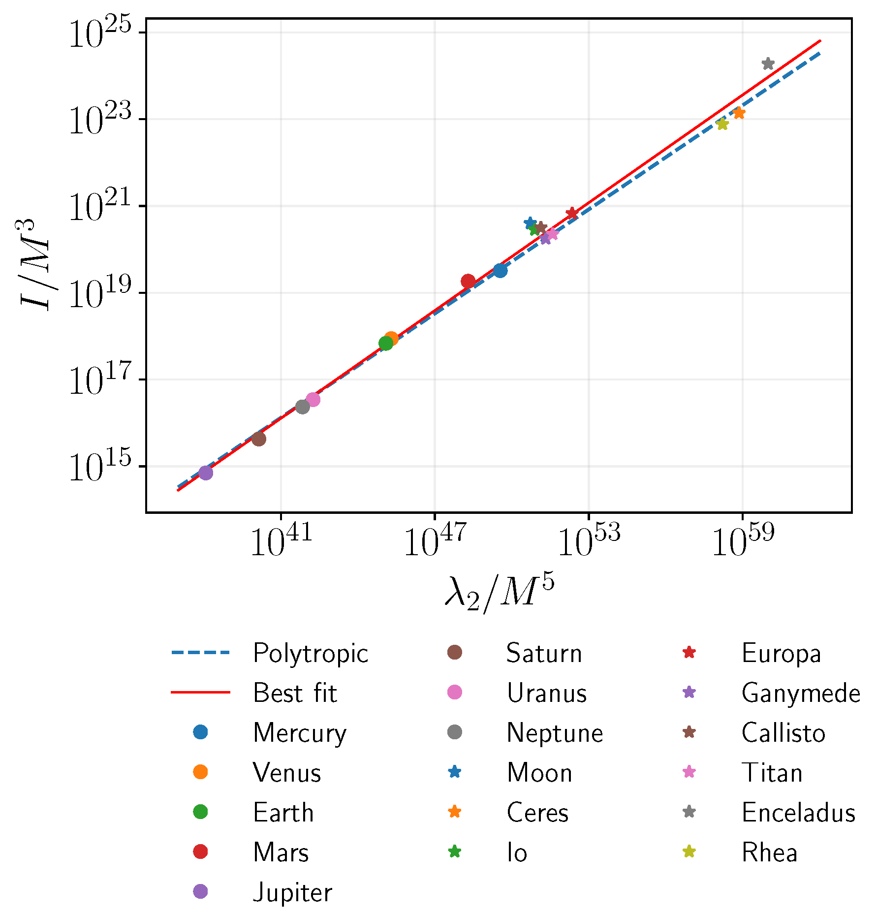
2.4. Checking Against the Planets in the Solar System

For NSs, verifying the I-Love universal relation through measurements remains challenging due to the lack of simultaneous observations of I and ${\lambda }_2$. However, for Newtonian stars, the I-Love universal relation can be validated using measurements from planets and moons within our solar system.

Table 1. Moment of inertia and tidal Love number for the planets and moons in the solar system. Intervals are used to indicate the uncertainties; central values of the intervals are plotted in Figure 6. The results marked with the asterisks are deduced based on models of the objects’ interior structures.

Object	$\mathit{M}\left[{10}^{22}\mathbf{kg}\right]$	$\mathit{R}\left[{10}^6\mathbf{m}\right]$	$\mathit{I}/\left({\mathit{MR}}^2\right)$	${\mathit{k}}_2$	Ref.
Mercury	$33.0$	$2.440$	$[0.328,0.338]$	$[0.544,0.594]$	[55,73]
Venus	$4.87\times {10}^2$	$6.052$	$[0.313,0.361]$	$[0.229,0.361]$	[74,75]
Earth	$5.97\times {10}^2$	$6.378$	$0.3307007$	$[0.3012,0.3014]$	[76,77]
Mars	$64.2$	$3.396$	$[0.3639,0.3649]$	$[0.163,0.175]$	[78,79]
Jupiter	$1.90\times {10}^5$	$71.49$	$[0.2749,0.2762]$ *	$[0.5299,0.5403]$ *	[56,80]
Saturn	$5.68\times {10}^4$	$60.27$	$[0.21,0.23]$	$[0.347,0.399]$	[57,81]
Uranus	$8.68\times {10}^3$	$25.56$	$[0.22,0.24]$ *	$[0.275,0.363]$ *	[58,82]
Neptune	$1.02\times {10}^4$	$24.76$	$[0.22,0.24]$ *	$[0.28,0.30]$ *	[59,82]
Moon	$7.35$	$1.737$	$[0.3927,0.3931]$	$[0.02394,0.02444]$	[83,84]
Ceres	$9.47\times {10}^{-2}$	$0.475$	$[0.373,0.390]$ *	$[1.15,1.50]$ *	[60,61]
Io	$8.93$	$1.822$	$[0.3765,0.3772]$ *	$[0.075,0.095]$ *	[62,63]
Europa	$4.80$	$1.561$	$[0.3523,0.3571]$ *	$[0.21,0.27]$ *	[64,65]
Ganymede	$14.8$	$2.631$	$[0.3087,0.3143]$ *	$[0.4,0.5]$ *	[64,66]
Callisto	$10.8$	$2.410$	$[0.3507,0.3591]$ *	$[0.083,0.58]$ *	[66,67]
Titan	$13.5$	$2.576$	$[0.3409,0.3419]$ *	$[0.514,0.749]$ *	[68,69]
Enceladus	$1.08\times {10}^{-2}$	$0.190$	$[0.3348,0.3352]$ *	$[0.01965,0.02035]$ *	[70]
Rhea	$0.231$	$0.7644$	$[0.3866,0.3956]$ *	$[1.378,1.458]$ *	[71]

provides the masses, radii, moment of inertia factors, and tidal Love numbers for the eight planets and some of their moons. While some moment of inertia factors and tidal Love numbers are not directly measured, they are theoretically inferred from models based on the current best understanding of these celestial objects [55,56,57,58,59,60,61,62,63,64,65,66,67,68,69,70,71,72]; these models are significantly more reliable but also have significantly more parameters than the simplistic model of spherical polytropic stars.

In Figure 6, we depict the data for the moment of inertia and tidal Love number of the celestial objects listed in Table 1, alongside the theoretical line of Equation (44). The trend of the data aligns well with the theoretical line, particularly for planets. A linear regression of the data in the logarithmic scale yields

$$\begin{array}{c}\hfill {log}_{10}\left({\displaystyle \frac{I}{M^3}}\right)=0.412{log}_{10}\left({\displaystyle \frac{{\lambda }_2}{M^5}}\right)-0.803,\end{array}$$

(45)

with an R-Squared value of $0.984$. The slope $0.412$ is slightly greater than the theoretical value $2/5$. This is likely because the planets and the moons are slightly oblate due to their rotations or tides from nearby bodies, so they have larger moments of inertia than spherical bodies of the same masses.

3. Summary

We numerically calculate the moment of inertia (I) and the tidal Love number (Love) for polytropic stars in both Newtonian gravity and GR. The I-Love relation varies within $1\%$ for different polytropic indices in Newtonian gravity and within $10\%$ for different polytropic indices in GR. The results explicitly demonstrate that the I-Love universal relation not only exists for compact stars but also exists for Newtonian stars.

We also compute the moment of inertia and the tidal Love number for realistic NSs and white dwarfs to compare with the polytropic stars. We find that the I-Love relation of the realistic NSs falls within $1\%$ of the I-Love relation of the $n\to 0$ polytropic case. For white dwarfs, their I-Love relation has a $10\%$ discrepancy away from the $n\to 0$ polytropic case when compared to the GR solution; surprisingly, the I-love relation for white dwarfs agrees better with the Newtonian result.

Finally, we collected measured and theoretically inferred data of the moment of inertia and the tidal Love number for 17 celestial bodies in our solar system to check the I-Love universal relation obtained for polytropic stars. The trend of the data follows the theoretical line well. The slope of the best-fit line of the data deviates from the theoretical value $2/5$ by only $3\%$, showing the adequacy of the theoretical I-Love universal relation in describing real planets and moons. Therefore, the I-Love universal relation provides a valuable tool for exploring exoplanets. Especially when combined with the Darwin–Radau equation [85], one can compute the moment of inertia and the tidal Love number of the exoplanet if its mass, spin frequency, equatorial radius, and polar radius are known. The moment of inertia and the tidal Love number are closely related to the interior structure and compositions of the planet. Knowing them helps build detailed models of the exoplanet and, thus, understand it better.

References

1. Yagi, K.; Yunes, N. I-Love-Q. Science 2013, 341, 365–368. [Google Scholar] [CrossRef] [PubMed]
2. Yagi, K.; Yunes, N. I-Love-Q Relations in Neutron Stars and their Applications to Astrophysics, Gravitational Waves and Fundamental Physics. Phys. Rev. D 2013, 88, 023009. [Google Scholar] [CrossRef]
3. Stein, L.C.; Yagi, K.; Yunes, N. Three-Hair Relations for Rotating Stars: Nonrelativistic Limit. Astrophys. J. 2014, 788, 15. [Google Scholar] [CrossRef]
4. Yagi, K. Multipole Love Relations. Phys. Rev. D 2014, 89, 043011, Erratum in Phys. Rev. D 2017, 96, 129904; Erratum in Phys. Rev. D 2018, 97, 129901. [Google Scholar] [CrossRef]
5. Yagi, K.; Kyutoku, K.; Pappas, G.; Yunes, N.; Apostolatos, T.A. Effective No-Hair Relations for Neutron Stars and Quark Stars: Relativistic Results. Phys. Rev. D 2014, 89, 124013. [Google Scholar] [CrossRef]
6. Pani, P.; Gualtieri, L.; Ferrari, V. Tidal Love numbers of a slowly spinning neutron star. Phys. Rev. D 2015, 92, 124003. [Google Scholar] [CrossRef]
7. Delsate, T. I-Love relations for irrotational stars. Phys. Rev. D 2015, 92, 124001. [Google Scholar] [CrossRef]
8. Bretz, J.; Yagi, K.; Yunes, N. Four-Hair Relations for Differentially Rotating Neutron Stars in the Weak-Field Limit. Phys. Rev. D 2015, 92, 083009. [Google Scholar] [CrossRef]
9. Yagi, K.; Yunes, N. Approximate Universal Relations for Neutron Stars and Quark Stars. Phys. Rept. 2017, 681, 1–72. [Google Scholar] [CrossRef]
10. Chan, T.K.; Sham, Y.H.; Leung, P.T.; Lin, L.M. Multipolar universal relations between f-mode frequency and tidal deformability of compact stars. Phys. Rev. D 2014, 90, 124023. [Google Scholar] [CrossRef]
11. Chirenti, C.; de Souza, G.H.; Kastaun, W. Fundamental oscillation modes of neutron stars: Validity of universal relations. Phys. Rev. D 2015, 91, 044034. [Google Scholar] [CrossRef]
12. Doneva, D.D.; Kokkotas, K.D. Asteroseismology of rapidly rotating neutron stars—An alternative approach. Phys. Rev. D 2015, 92, 124004. [Google Scholar] [CrossRef]
13. Krüger, C.J.; Kokkotas, K.D. Fast Rotating Relativistic Stars: Spectra and Stability without Approximation. Phys. Rev. Lett. 2020, 125, 111106. [Google Scholar] [CrossRef]
14. Pappas, G.; Apostolatos, T.A. Effectively universal behavior of rotating neutron stars in general relativity makes them even simpler than their Newtonian counterparts. Phys. Rev. Lett. 2014, 112, 121101. [Google Scholar] [CrossRef]
15. Chakrabarti, S.; Delsate, T.; Gürlebeck, N.; Steinhoff, J. I-Q relation for rapidly rotating neutron stars. Phys. Rev. Lett. 2014, 112, 201102. [Google Scholar] [CrossRef]
16. Manoharan, P.; Kokkotas, K.D. Finding universal relations using statistical data analysis. Phys. Rev. D 2024, 109, 103033. [Google Scholar] [CrossRef]
17. Maselli, A.; Cardoso, V.; Ferrari, V.; Gualtieri, L.; Pani, P. Equation-of-state-independent relations in neutron stars. Phys. Rev. D 2013, 88, 023007. [Google Scholar] [CrossRef]
18. Vretinaris, S.; Stergioulas, N.; Bauswein, A. Empirical relations for gravitational-wave asteroseismology of binary neutron star mergers. Phys. Rev. D 2020, 101, 084039. [Google Scholar] [CrossRef]
19. Manoharan, P.; Krüger, C.J.; Kokkotas, K.D. Universal relations for binary neutron star mergers with long-lived remnants. Phys. Rev. D 2021, 104, 023005. [Google Scholar] [CrossRef]
20. Guedes, V.; Lau, S.Y.; Chirenti, C.; Yagi, K. Broadening of universal relations at the birth and death of a neutron star. Phys. Rev. D 2024, 109, 083040. [Google Scholar] [CrossRef]
21. Yagi, K.; Stein, L.C.; Pappas, G.; Yunes, N.; Apostolatos, T.A. Why I-Love-Q: Explaining why universality emerges in compact objects. Phys. Rev. D 2014, 90, 063010. [Google Scholar] [CrossRef]
22. Bekenstein, J.D. Novel ‘‘no-scalar-hair’’ theorem for black holes. Phys. Rev. D 1995, 51, R6608. [Google Scholar] [CrossRef] [PubMed]
23. Doneva, D.D.; Yazadjiev, S.S.; Stergioulas, N.; Kokkotas, K.D. Breakdown of I-Love-Q universality in rapidly rotating relativistic stars. Astrophys. J. Lett. 2013, 781, L6. [Google Scholar] [CrossRef]
24. Taylor, A.; Yagi, K.; Arras, P.L. I–Love–Q relations for realistic white dwarfs. Mon. Not. Roy. Astron. Soc. 2020, 492, 978–992. [Google Scholar] [CrossRef]
25. Chen, K.; Lin, L.M. Fully general relativistic simulations of rapidly rotating quark stars: Oscillation modes and universal relations. Phys. Rev. D 2023, 108, 064007. [Google Scholar] [CrossRef]
26. Silva, H.O.; Macedo, C.F.B.; Berti, E.; Crispino, L.C.B. Slowly rotating anisotropic neutron stars in general relativity and scalar–tensor theory. Class. Quant. Grav. 2015, 32, 145008. [Google Scholar] [CrossRef]
27. Yagi, K.; Yunes, N. I-Love-Q anisotropically: Universal relations for compact stars with scalar pressure anisotropy. Phys. Rev. D 2015, 91, 123008. [Google Scholar] [CrossRef]
28. Martinon, G.; Maselli, A.; Gualtieri, L.; Ferrari, V. Rotating protoneutron stars: Spin evolution, maximum mass, and I-Love-Q relations. Phys. Rev. D 2014, 90, 064026. [Google Scholar] [CrossRef]
29. Yeung, C.H.; Lin, L.M.; Andersson, N.; Comer, G. The I-Love-Q Relations for Superfluid Neutron Stars. Universe 2021, 7, 111. [Google Scholar] [CrossRef]
30. Laskos-Patkos, P.; Koliogiannis, P.S.; Kanakis-Pegios, A.; Moustakidis, C.C. Universal relations and finite temperature neutron stars. HNPS Adv. Nucl. Phys. 2023, 29, 94–99. [Google Scholar] [CrossRef]
31. Doneva, D.D.; Yazadjiev, S.S.; Staykov, K.V.; Kokkotas, K.D. Universal I-Q relations for rapidly rotating neutron and strange stars in scalar-tensor theories. Phys. Rev. D 2014, 90, 104021. [Google Scholar] [CrossRef]
32. Doneva, D.D.; Pappas, G. Universal Relations and Alternative Gravity Theories. Astrophys. Space Sci. Libr. 2018, 457, 737–806. [Google Scholar] [CrossRef]
33. Gupta, T.; Majumder, B.; Yagi, K.; Yunes, N. I-Love-Q Relations for Neutron Stars in dynamical Chern Simons Gravity. Class. Quant. Grav. 2018, 35, 025009. [Google Scholar] [CrossRef]
34. Pappas, G.; Doneva, D.D.; Sotiriou, T.P.; Yazadjiev, S.S.; Kokkotas, K.D. Multipole moments and universal relations for scalarized neutron stars. Phys. Rev. D 2019, 99, 104014. [Google Scholar] [CrossRef]
35. Hu, Z.; Gao, Y.; Xu, R.; Shao, L. Scalarized neutron stars in massive scalar-tensor gravity: X-ray pulsars and tidal deformability. Phys. Rev. D 2021, 104, 104014. [Google Scholar] [CrossRef]
36. Xu, R.; Gao, Y.; Shao, L. Neutron stars in massive scalar-Gauss-Bonnet gravity: Spherical structure and time-independent perturbations. Phys. Rev. D 2022, 105, 024003. [Google Scholar] [CrossRef]
37. Silva, H.O.; Sakstein, J.; Gualtieri, L.; Sotiriou, T.P.; Berti, E. Spontaneous scalarization of black holes and compact stars from a Gauss-Bonnet coupling. Phys. Rev. Lett. 2018, 120, 131104. [Google Scholar] [CrossRef]
38. Doneva, D.D.; Yazadjiev, S.S. New Gauss-Bonnet Black Holes with Curvature-Induced Scalarization in Extended Scalar-Tensor Theories. Phys. Rev. Lett. 2018, 120, 131103. [Google Scholar] [CrossRef]
39. Antoniou, G.; Bakopoulos, A.; Kanti, P. Evasion of No-Hair Theorems and Novel Black-Hole Solutions in Gauss-Bonnet Theories. Phys. Rev. Lett. 2018, 120, 131102. [Google Scholar] [CrossRef]
40. Sham, Y.H.; Chan, T.K.; Lin, L.M.; Leung, P.T. Unveiling the universality of I-Love-Q relations. Astrophys. J. 2015, 798, 121. [Google Scholar] [CrossRef]
41. Yip, K.L.S.; Leung, P.T. Tidal Love numbers and moment-Love relations of polytropic stars. Mon. Not. Roy. Astron. Soc. 2017, 472, 4965–4981. [Google Scholar] [CrossRef]
42. Poisson, E.; Will, C.M. Gravity: Newtonian, Post-Newtonian, Relativistic; Cambridge University Press: Cambridge, UK, 2014. [Google Scholar] [CrossRef]
43. Thorne, K.S. Multipole Expansions of Gravitational Radiation. Rev. Mod. Phys. 1980, 52, 299–339. [Google Scholar] [CrossRef]
44. Hartle, J.B. Slowly rotating relativistic stars. 1. Equations of structure. Astrophys. J. 1967, 150, 1005–1029. [Google Scholar] [CrossRef]
45. Hinderer, T. Tidal Love numbers of neutron stars. Astrophys. J. 2008, 677, 1216–1220. [Google Scholar] [CrossRef]
46. Damour, T.; Nagar, A. Relativistic tidal properties of neutron stars. Phys. Rev. D 2009, 80, 084035. [Google Scholar] [CrossRef]
47. Binnington, T.; Poisson, E. Relativistic theory of tidal Love numbers. Phys. Rev. D 2009, 80, 084018. [Google Scholar] [CrossRef]
48. Regge, T.; Wheeler, J.A. Stability of a Schwarzschild singularity. Phys. Rev. 1957, 108, 1063–1069. [Google Scholar] [CrossRef]
49. Andersson, N.; Comer, G.L. Relativistic fluid dynamics: Physics for many different scales. Living Rev. Rel. 2007, 10, 1. [Google Scholar] [CrossRef]
50. Chabanat, E.; Meyer, J.; Bonche, P.; Schaeffer, R.; Haensel, P. A Skyrme parametrization from subnuclear to neutron star densities. Nucl. Phys. A 1997, 627, 710–746. [Google Scholar] [CrossRef]
51. Chabanat, E.; Bonche, P.; Haensel, P.; Meyer, J.; Schaeffer, R. A Skyrme parametrization from subnuclear to neutron star densities. 2. Nuclei far from stablities. Nucl. Phys. A 1998, 635, 231–256, Erratum in Nucl. Phys. A 1998, 643, 441–441. [Google Scholar] [CrossRef]
52. Chan, T.K.; Chan, A.P.O.; Leung, P.T. I-Love relations for incompressible stars and realistic stars. Phys. Rev. D 2015, 91, 044017. [Google Scholar] [CrossRef]
53. Chan, T.K.; Chan, A.P.O.; Leung, P.T. Universality and stationarity of the I-Love relation for self-bound stars. Phys. Rev. D 2016, 93, 024033. [Google Scholar] [CrossRef]
54. Staykov, K.V.; Doneva, D.D.; Yazadjiev, S.S. Moment-of-inertia-compactness universal relations in scalar-tensor theories and R2 gravity. Phys. Rev. D 2016, 93, 084010. [Google Scholar] [CrossRef]
55. Genova, A.; Goossens, S.; Mazarico, E.; Lemoine, F.G.; Neumann, G.A.; Kuang, W.; Sabaka, T.J.; Hauck, S.A.; Smith, D.E.; Solomon, S.C.; et al. Geodetic Evidence That Mercury Has A Solid Inner Core. Geophys. Res. Lett. 2019, 46, 3625–3633. [Google Scholar] [CrossRef]
56. Wahl, S.M.; Hubbard, W.B.; Militzer, B. Tidal Response of Preliminary Jupiter Model. Astrophys. J. 2016, 831, 14. [Google Scholar] [CrossRef]
57. Fortney, J.J.; Helled, R.; Nettelmann, N.; Stevenson, D.J.; Marley, M.S.; Hubbard, W.B.; Iess, L. The Interior of Saturn. In Saturn in the 21st Century; Baines, K.H., Flasar, F.M., Krupp, N., Stallard, T., Eds.; Cambridge University Press: Cambridge, UK, 2018; pp. 44–68. [Google Scholar] [CrossRef]
58. Stixrude, L.; Baroni, S.; Grasselli, F. Thermal and Tidal Evolution of Uranus with a Growing Frozen Core. Planet. Sci. J. 2021, 2, 222. [Google Scholar] [CrossRef]
59. James, D.A.; Stixrude, L. Thermal and Tidal Evolution of Ice Giants with Growing Frozen Cores: The Case of Neptune. Space Sci. Rev. 2024, 220, 21. [Google Scholar] [CrossRef]
60. McCord, T.B.; Sotin, C. Ceres: Evolution and current state. J. Geophys. Res. (Planets) 2005, 110, E05009. [Google Scholar] [CrossRef]
61. Mao, X.; McKinnon, W.B. Faster paleospin and deep-seated uncompensated mass as possible explanations for Ceres’ present-day shape and gravity. Icarus 2018, 299, 430–442. [Google Scholar] [CrossRef]
62. Zharkov, V.N.; Gudkova, T.V. Models, figures and gravitational moments of Jupiter’s satellite Io: Effects of the second order approximation. Planet. Space Sci. 2010, 58, 1381–1390. [Google Scholar] [CrossRef]
63. Kervazo, M.; Tobie, G.; Choblet, G.; Dumoulin, C.; Běhounková, M. Inferring Io’s interior from tidal monitoring. Icarus 2022, 373, 114737. [Google Scholar] [CrossRef]
64. Schubert, G.; Anderson, J.D.; Spohn, T.; McKinnon, W.B. Interior composition, structure and dynamics of the Galilean satellites. In Jupiter. The Planet, Satellites and Magnetosphere; Bagenal, F., Dowling, T.E., McKinnon, W.B., Eds.; Cambridge University Press: Cambridge, UK, 2004; Volume 1, pp. 281–306. [Google Scholar]
65. Petricca, F.; Tharimena, S.; Melini, D.; Spada, G.; Bagheri, A.; Styczinski, M.J.; Vance, S.D. Exploring the tidal responses of ocean worlds with PyALMA3. Icarus 2024, 417, 116120. [Google Scholar] [CrossRef]
66. Van Hoolst, T.; Tobie, G.; Vallat, C.; Altobelli, N.; Bruzzone, L.; Cao, H.; Dirkx, D.; Genova, A.; Hussmann, H.; Iess, L.; et al. Geophysical Characterization of the Interiors of Ganymede, Callisto and Europa by ESA’s JUpiter ICy moons Explorer. Space Sci. Rev. 2024, 220, 54. [Google Scholar] [CrossRef]
67. Moore, W.B.; Schubert, G. The tidal response of Ganymede and Callisto with and without liquid water oceans. Icarus 2003, 166, 223–226. [Google Scholar] [CrossRef]
68. Iess, L.; Jacobson, R.A.; Ducci, M.; Stevenson, D.J.; Lunine, J.I.; Armstrong, J.W.; Asmar, S.W.; Racioppa, P.; Rappaport, N.J.; Tortora, P. The Tides of Titan. Science 2012, 337, 457. [Google Scholar] [CrossRef]
69. Durante, D.; Hemingway, D.J.; Racioppa, P.; Iess, L.; Stevenson, D.J. Titan’s gravity field and interior structure after Cassini. Icarus 2019, 326, 123–132. [Google Scholar] [CrossRef]
70. Genova, A.; Parisi, M.; Gargiulo, A.M.; Petricca, F.; Andolfo, S.; Torrini, T.; Del Vecchio, E.; Glein, C.R.; Cable, M.L.; Phillips, C.B.; et al. Gravity Investigation to Characterize Enceladus’s Ocean and Interior. Planet. Sci. J. 2024, 5, 40. [Google Scholar] [CrossRef]
71. Anderson, J.D.; Schubert, G. Saturn’s satellite Rhea is a homogeneous mix of rock and ice. Geophys. Res. Lett. 2007, 34, L02202. [Google Scholar] [CrossRef]
72. Stevenson, D.J. Jupiter’s Interior as Revealed by Juno. Annu. Rev. Earth Planet. Sci. 2020, 48, 465–489. [Google Scholar] [CrossRef]
73. Verma, A.K.; Margot, J.L. Mercury’s gravity, tides, and spin from MESSENGER radio science data. J. Geophys. Res. (Planets) 2016, 121, 1627–1640. [Google Scholar] [CrossRef]
74. Konopliv, A.S.; Yoder, C.F. Venusian k 2 tidal Love number from Magellan and PVO tracking data. Geophys. Res. Lett. 1996, 23, 1857–1860. [Google Scholar] [CrossRef]
75. Margot, J.L.; Campbell, D.B.; Giorgini, J.D.; Jao, J.S.; Snedeker, L.G.; Ghigo, F.D.; Bonsall, A. Spin state and moment of inertia of Venus. Nat. Astron. 2021, 5, 676–683. [Google Scholar] [CrossRef]
76. Williams, J.G. Contribution to the Earth’s Obliquity Rate, Precession, and Nutation. Astron. J. 1994, 108, 711. [Google Scholar] [CrossRef]
77. Jagoda, M.; Rutkowska, M. Estimation of the Love numbers: K 2, k 3 using SLR data of the LAGEOS1, LAGEOS2, STELLA and STARLETTE satellites. Acta Geod. Et Geophys. 2016, 51, 493–504. [Google Scholar] [CrossRef]
78. Konopliv, A.S.; Asmar, S.W.; Folkner, W.M.; Karatekin, Ö.; Nunes, D.C.; Smrekar, S.E.; Yoder, C.F.; Zuber, M.T. Mars high resolution gravity fields from MRO, Mars seasonal gravity, and other dynamical parameters. Icarus 2011, 211, 401–428. [Google Scholar] [CrossRef]
79. Konopliv, A.S.; Park, R.S.; Rivoldini, A.; Baland, R.M.; Le Maistre, S.; Van Hoolst, T.; Yseboodt, M.; Dehant, V. Detection of the Chandler Wobble of Mars From Orbiting Spacecraft. Geophys. Res. Lett. 2020, 47, e90568. [Google Scholar] [CrossRef]
80. Ni, D. Empirical models of Jupiter’s interior from Juno data. Moment of inertia and tidal Love number k2. Astron. Astrophys. 2018, 613, A32. [Google Scholar] [CrossRef]
81. Lainey, V.; Dewberry, J.W.; Fuller, J.; Cooper, N.; Rambaux, N.; Zhang, Q. Tidal frequency dependence of the Saturnian k2 Love number. Astron. Astrophys. 2024, 684, L3. [Google Scholar] [CrossRef]
82. Yoder, C.F. Astrometric and Geodetic Properties of Earth and the Solar System. In Global Earth Physics: A Handbook of Physical Constants; Ahrens, T.J., Ed.; American Geophysical Union: Washington, DC, USA, 1995; p. 1. [Google Scholar]
83. Williams, J.G.; Newhall, X.X.; Dickey, J.O. Lunar moments, tides, orientation, and coordinate frames. Planet. Space Sci. 1996, 44, 1077–1080. [Google Scholar] [CrossRef]
84. Williams, J.G.; Konopliv, A.S.; Boggs, D.H.; Park, R.S.; Yuan, D.N.; Lemoine, F.G.; Goossens, S.; Mazarico, E.; Nimmo, F.; Weber, R.C.; et al. Lunar interior properties from the GRAIL mission. J. Geophys. Res. (Planets) 2014, 119, 1546–1578. [Google Scholar] [CrossRef]
85. Bourda, G.; Capitaine, N. Precession, nutation, and space geodetic determination of the Earth’s variable gravity field. Astron. Astrophys. 2004, 428, 691–702. [Google Scholar] [CrossRef]
86. Shapiro, S.L.; Teukolsky, S.A. Black Holes, White Dwarfs, and Neutron Stars: The Physics of Compact Objects; Wiley-VCH: Weinheim, Germany, 1983. [Google Scholar] [CrossRef]
87. Chandrasekhar, S. An Introduction to the Study of Stellar Structure; Dover Publications: Mineola, NY, USA, 2010. [Google Scholar]
88. Boshkayev, K.; Quevedo, H.; Zhami, B. I -Love- Q relations for white dwarf stars. Mon. Not. Roy. Astron. Soc. 2017, 464, 4349–4359. [Google Scholar] [CrossRef]
Figure 1. The mass–radius relation for polytropic stars. The dashed lines are the Newtonian results, and the solid lines are the results using GR. Notice that the Newtonian lines extend to infinite mass.
Galaxies 13 00075 g001
Figure 2. Upper panel: the moment of inertia factor I / ( M R 2 ) versus the mass of the polytropic star. Lower panel: the tidal Love number k 2 versus the mass of the polytropic star. The dashed lines are the Newtonian results, and the solid lines are the results using GR. Notice that the Newtonian results do not change with the mass of the star.
Galaxies 13 00075 g002
Figure 3. Upper panel: The I-Love universal relation in Newtonian gravity (dashed lines) and in GR (solid lines). Lower panel: Relative discrepancies between each line and the n = 1 / 99 lines in Newtonian gravity and in GR, correspondingly. The results using the SLy4 EOS, which is a realistic EOS for NSs, and the zero-temperature EOS for white dwarfs are also plotted for comparison.
Galaxies 13 00075 g003
Figure 4. An example of non-universal relation: I / R 3 versus λ 2 / R 5 . The dashed lines are the Newtonian results, and the solid lines are the results using GR. The result of NSs (SLy4) is also plotted for comparison. The result of white dwarfs has values of I / R 3 that are too small to show in the plot.
Galaxies 13 00075 g004
Figure 5. An example of non-universal relation: the compactness C versus λ 2 / M 5 . The dashed lines are the Newtonian results, and the solid lines are the results using GR. The results of NSs (SLy4) and white dwarfs are also plotted for comparison. Notice that the compactness of the Newtonian polytropic star extends to infinity.
Galaxies 13 00075 g005
Figure 6. The theoretical I-Love universal relation checked against the measurements of the solar-system celestial bodies.
Galaxies 13 00075 g006