Nonlinear Stability of the Bardeen–De Sitter Wormhole in f(R) Gravity

Abstract

This paper discusses the nonlinear stability of a thin-shell wormhole from a regular black hole in Bardeen–de Sitter spacetime in the $f\left(R\right)$ gravity framework. The stability is examined under the linear perturbation about static solution and a nonlinear variable equation of state, such as the modified generalized Chaplygin gas. The stability solutions for a suitable choice of different parameters included in the variable equation of state and $f\left(R\right)$ gravity models, as well as the metric space–time, are illustrated.

1. Introduction

In 1988, Morris and Thorne [1] analyzed traversable wormholes as a geometrical object which, by joining two manifolds, may be similar or different. Afterward, Visser [2] investigated the concept of thin-shell wormholes (TSWs) formed by Visser’s cutting and pasting two spacetimes. The construction of these wormholes required the presence of an exotic matter at the wormhole throat, which violates energy conditions [3]. Various forms of equation of state (EoS), such as linear and nonlinear EoS, have been discussed in the framework of TSWs [4,5,6].

Furthermore, Bardeen [7] introduced the concept of a non-singular regular black hole (RBH) model, called the Bardeen black hole model, which has an event horizon and precludes singularity at the origin. Afterward, several authors discussed the other RBH models depending on the conception of the Bardeen model.

For instance, Ayon-Beato and Garcia [8] studied a non-linear magnetic monopole via the Bardeen model. Recently, Shamir [9] analyzed the charged massive compact star under conformal motion via Bardeen geometry. Sharif and Javed [10] studied the Bardeen wormholes’ stability, and also analyzed the anti-de Sitter Bardeen TSWs’ stability [11]. Similarly, Haywad [12] investigated a similar stability type model of RBH. Furthermore, Rahaman et al. [13] studied the TSW stability formed from charged RBH. In addition, Eid [14] discussed the dynamics of Bardeen–de Sitter TSWs and stability. Further, Fernando [15] analyzed the Bardeen–de Sitter BH properties. Li et al. [16] discussed anti-de Sitter–Bardeen BH thermodynamics. Alshal [17] analyzed the Bardeen–de Sitter TSWs’ stability.

The observed phenomenon of the accelerated expansion of the universe may be explained according to the modified gravity theories or the dark energy models [18,19]. In 1970, Buchdal [20] introduced the concept of a modified theory of $f\left(R\right)$ gravity as a modified version of general relativity. This modification is based on replacing the action $R$ with an arbitrary scalar curvature function of $f\left(R\right)$ [21,22,23].

In several articles, the stability of TSWs and BHs in the framework of $f\left(R\right)$ theory has been discussed. For instance, Shamir and Fayyaz [24] discussed a wormhole model in $f\left(R\right)$ theory via the Karmarkar condition. Godani [25] discussed the linear and nonlinear stability of charged TSWs in $f\left(R\right)$ gravity and studied TSWs in a nonlinear $f\left(R\right)$ theory [26]. Furthermore, Samanta and Godani [27] studied the stability of $f\left(R\right)$ models with physical parameters. Shamir and Malik [28] studied the compact Bardeen stars in $f\left(R\right)$ theory. Also, Eid [29] analyzed the stability of TSW in $f\left(R\right)$ gravity. Godani [30] discussed the Heyward wormhole stability in $f\left(R\right)$ gravity, and he also studied the Bardeen wormhole stability in the theory of $f\left(R\right)$ [31].

This article discusses the Bardeen–de Sitter TSW stability in the theory of $f\left(R\right)$ through linear perturbation via a nonlinear EoS, such as the variable modified generalized Chaplygin gas (VMGCG). Section 2 presents a short description of the Bardeen–de Sitter TSW formalism in f(R) gravity. Section 3 addresses stability analysis through linear perturbation via a quadratic–cubic model of $f\left(R\right)$ gravity. In Section 4, a remarkable conclusion is considered.

2. Bardeen–De Sitter Formalism

The Bardeen–de Sitter BH metric is described by [15]

$$d{s}_{\pm }^2=G_{\pm }^{-1}d{r}_{\pm }^2-G_{\pm }d{t}_{\pm }^2+h_{\pm }d{\mathsf{\Omega }}_{\pm }^2,$$

(1)

with

$$G_{\pm }\left(r_{\pm }\right)=1-{\displaystyle \frac{2m_{\pm }{r}_{\pm }^2}{{\left(r_{\pm }^2+q_{\pm }^2\right)}^{3/2}}}-{\displaystyle \frac{1}{3}}{r}_{\pm }^2{\mathsf{\Lambda }}_{\pm }, h_{\pm }\left(r_{\pm }\right)=r_{\pm }^2,$$

(2)

and $d{\mathsf{\Omega }}_{\pm }^2=\left(d{\theta }_{\pm }^2+{\mathit{sin}}^2{\theta }_{\pm }d{\phi }_{\pm }^2\right)$.

In this metric, $q_{\pm }$, $m_{\pm }$, and ${\mathsf{\Lambda }}_{\pm }$ denote the charge, mass, and cosmological constant of a black hole for the exterior (+) and interior (−) regions, separately. Let ${\mathrm{m}}_{-}={\mathrm{m}}_{+}=\mathrm{m}$, ${\mathsf{\Lambda }}_{+}={\mathsf{\Lambda }}_{-}=\mathsf{\Lambda }$ and $\mathrm{q}={\mathrm{q}}_{-}={\mathrm{q}}_{+}$. According to Visser’s approach (cut and paste), two identical copies of manifold $M^{\pm }$ ($M=M^{-}\cup M^{+}$) can be glued together at their hypersurface Σ (where $\mathsf{\Sigma }={\mathsf{\Sigma }}^{-}\cup {\mathsf{\Sigma }}^{+}$ represents a throat that connects both manifolds $M^{\pm }$). Furthermore, the evolution time of the shell is described by the relation $r_{\pm }=b\left(\tau \right)$, with the proper time $\tau$. Then, the metric induced on the boundaries $\Sigma$ is described by

$$d{s}^2=-d{\tau }^2+h\left(b\right)d{\mathsf{\Omega }}^2.$$

(3)

Moreover, the extrinsic curvature $K_{ij}^{\pm }$ of the two regions across Σ [32] is described by

$$K_{ij}^{\pm }=-n_{\mu }^{\pm }{\left.\left({\displaystyle \frac{{\partial }^2{Y}_{\pm }^{\mu }}{\partial {\zeta }^i\partial {\zeta }^j}}+{\Gamma }_{\alpha \beta }^{\mu }{\displaystyle \frac{\partial Y_{\pm }^{\alpha }}{\partial {\zeta }^i}}{\displaystyle \frac{\partial Y_{\pm }^{\beta }}{\partial {\zeta }^j}}\right)\right|}_{\Sigma },$$

(4)

where ${\zeta }^i$ and $Y_{\pm }^{\mu }$ are the coordinates on Σ and in $M^{\pm }$, respectively. Also, ${\mathsf{\Gamma }}_{\alpha \beta }^{\mu }$ and $n_{\mu }^{\pm }$ represent the Christoffel symbols and four-unit normal vector. Furthermore, Equations (2) and (4) can be used to obtain

$$K_{\tau \tau }^{\pm }=\mp {\displaystyle \frac{2\ddot{b}+\acute{G}}{2\sqrt{{\dot{b}}^2+G}}},K_{\theta \theta }^{\pm }=\pm {\displaystyle \frac{h\prime }{2h}}\sqrt{G+{\dot{b}}^2}\equiv K_{\phi \phi }^{\pm }.$$

(5)

where dot and prime represent the derivative with regard to $\tau$ and $b$, respectively.

Afterward, the field equation in the theory $f(R)$ [33] is described by

$$4\pi t_{ij}=-f^{\prime }\left(R\right)\left[K_{ij}\right],$$

(6)

where $t_{ij}=\left(\sigma ,p_{\theta },p_{\phi }\right)$ represents the intrinsic stress–energy tensor, with energy density $\sigma$ and principal pressures ($p_{\theta }$, $p_{\phi }$). Moreover, the continuity conditions $\left[h_j^i\right]=0$ and $\left[K_j^i\right]=0$ must hold [34]. Consequently, the constraint condition $\left[K_i^i\right]=0$ and Equation (5) can be used to obtain

$$\ddot{b}=-{\displaystyle \frac{1}{2}}{G}^{\prime }-{\displaystyle \frac{h^{\prime }}{h}}({\dot{b}}^2+G).$$

(7)

Therefore, (5) can be inserted into (6) to obtain

$$\sigma ={\displaystyle \frac{f_R}{4\pi }}\left({\displaystyle \frac{2\ddot{b}+G^{\prime }}{\sqrt{{\dot{b}}^2+G}}}\right),.$$

(8)

$$p\equiv p_{\theta }\equiv p_{\phi }=-{\displaystyle \frac{{h^{\prime }f}_R}{4\pi h}}\sqrt{{\dot{b}}^2+G}.$$

(9)

In addition, inserting Equation (7) into (8) gives

$$\sigma =-{\displaystyle \frac{h^{\prime }{f}_R}{2\pi h}}\sqrt{{\dot{b}}^2+G},$$

(10)

where $f_R={\displaystyle \frac{df\left(R\right)}{dR}}$. Consequently, the single dynamical equation of motion, derived from Equation (10), becomes

$${\dot{b}}^2+\psi (b)=0,$$

(11)

where $\psi \left(b\right)$ represents the effective potential and is written in the form

$$\psi (b)=G-{\left({\displaystyle \frac{2\pi \sigma h}{h^{\prime }{f}_R}}\right)}^2.$$

(12)

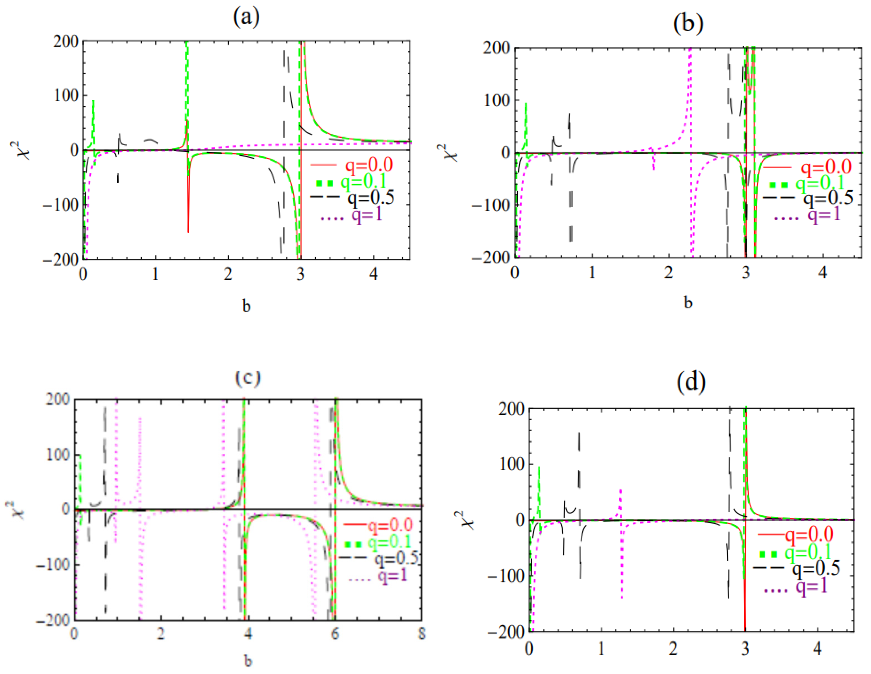
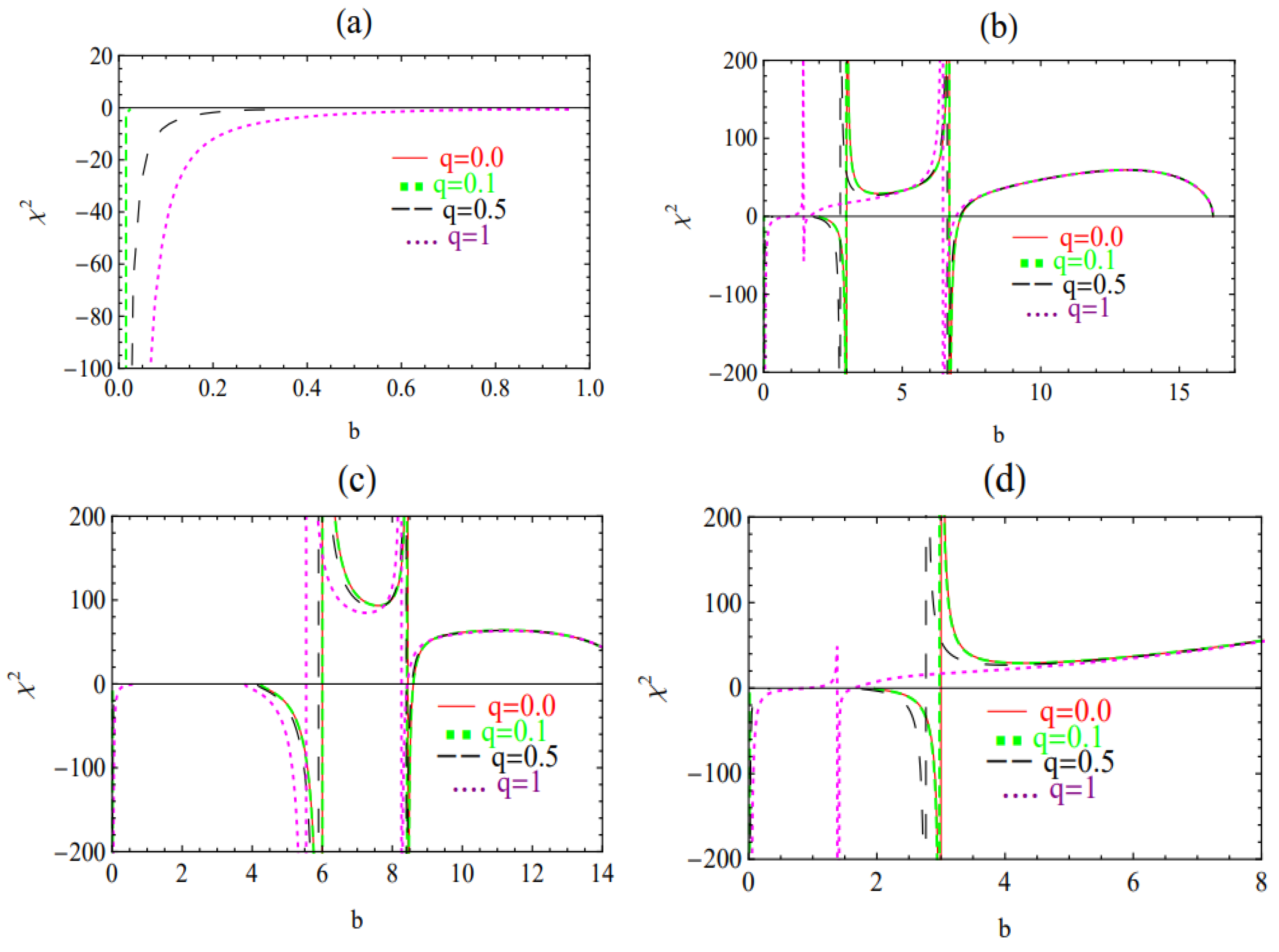
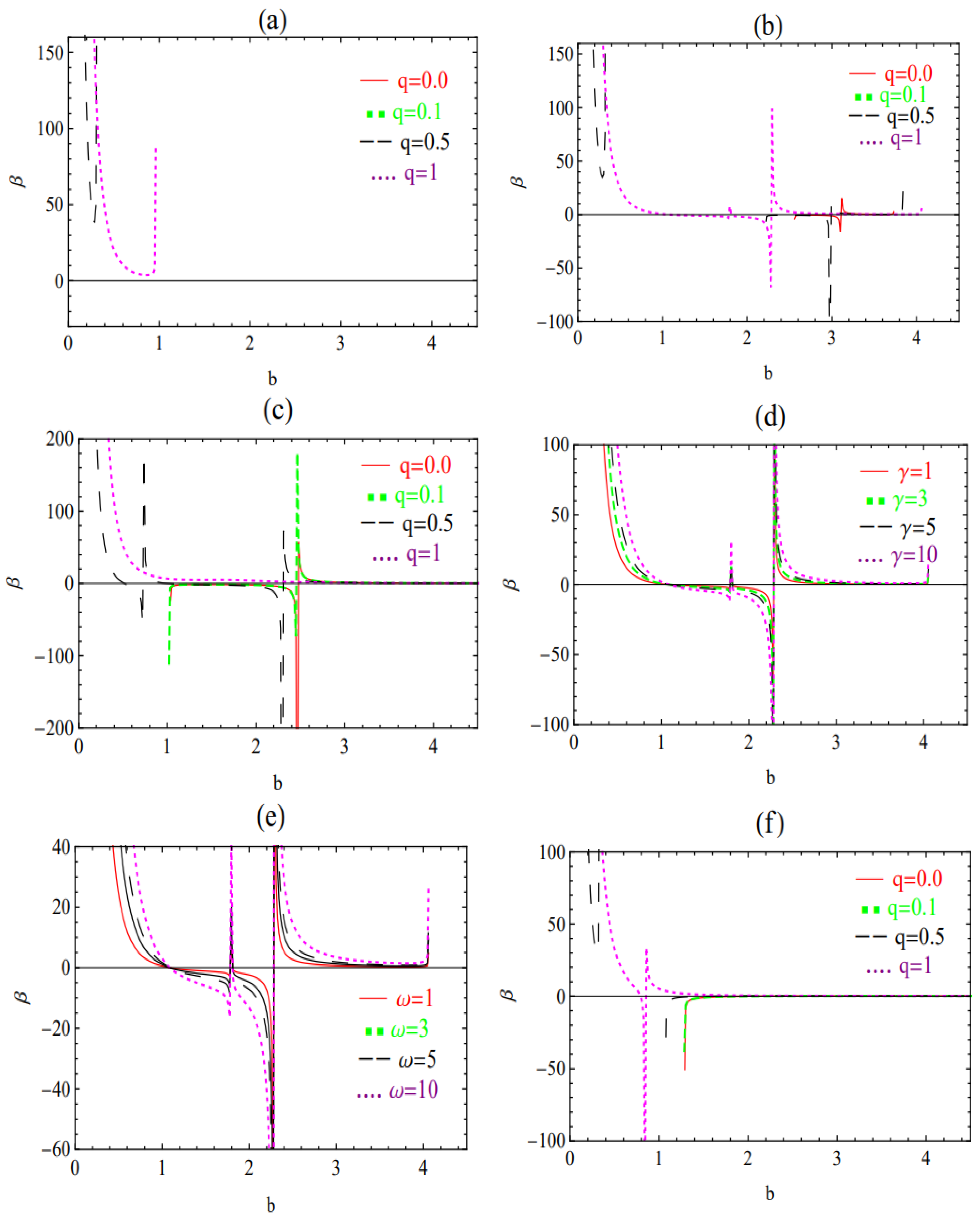
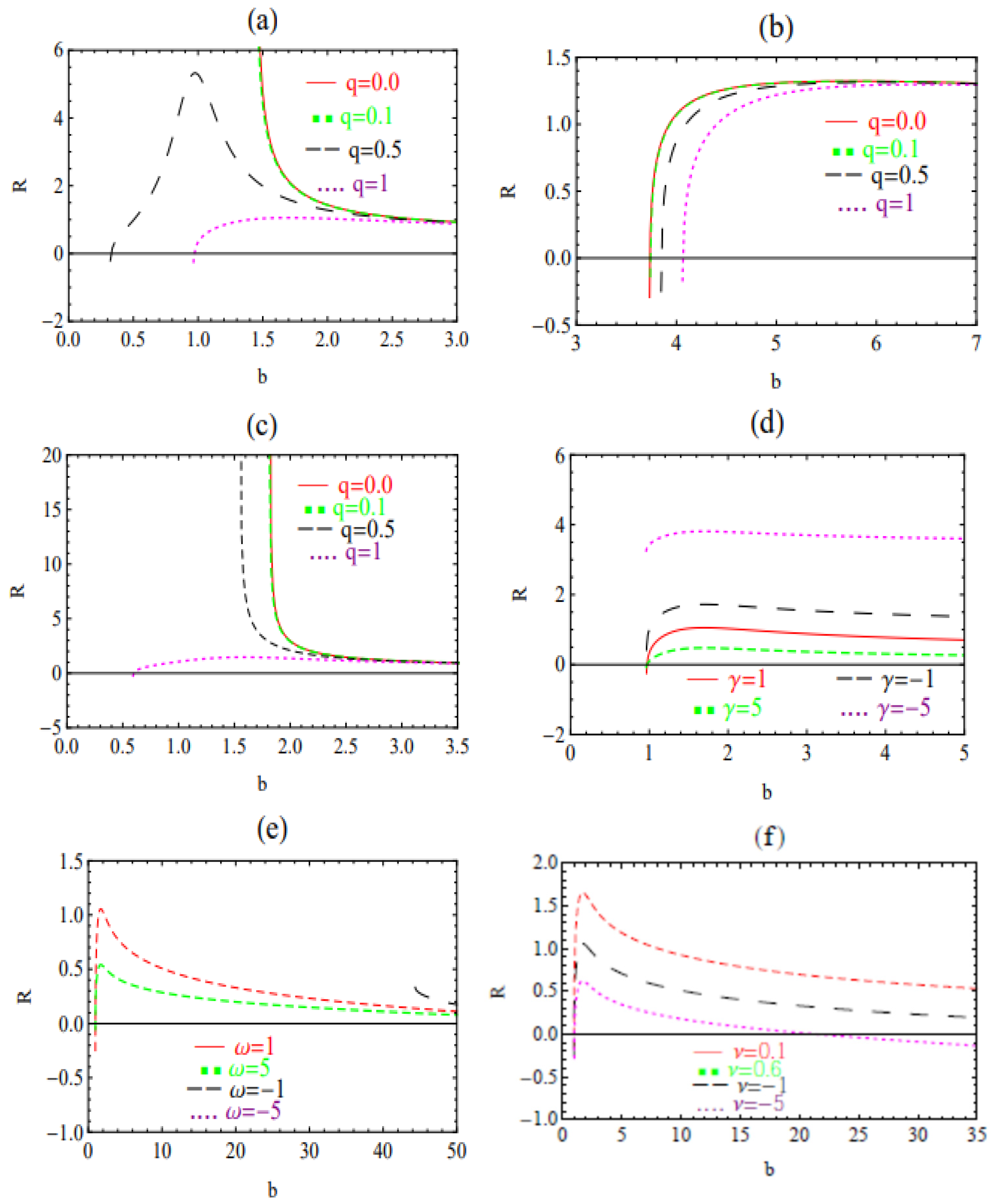
3. Stability Analysis

Accordingly, the equation of state is of great importance in order to analyze the stability of TSW and violation of energy conditions. It is clear from Equation (10) that if $f_R>0$, then the negative of $\sigma <0$ indicates the existence of exotic matter at the throat of the wormhole, which means that the presence of a repulsive gravitational force prevents it from contracting. It is observed that the matter distribution at the throat violates both the weak energy condition ($\sigma \ge 0$, $\sigma +p\ge 0$) and the null energy condition ($\sigma +p\ge 0$), due to the negativity of σ. It also violates the strong energy condition that requires ($\sigma +3p\ge 0$) [25].

Consequently, due to the negativity of energy density (10), and in order to study the dynamical characterization, we assumed exotic matter EoS, such as variable modified generalized Chaplygin gas (VMGCG) which is described by [35,36],

$$p(\sigma ,b)=\nu \sigma -{\displaystyle \frac{\mu }{{b^n\sigma }^{\alpha }}},$$

(13)

where $\mu >0,$ $\upsilon <0$, $0\le n\le 1$ and $0<\alpha \le 1$ are EoS parameters.

In addition, from Equation (13), different types of EoS are recovered, such as a variable generalized Chaplygin gas, which is recovered when $\nu =0$ is used, and Chaplygin gas is recovered with ($\nu =0$ and $\alpha =1$) [37,38], while the phantom energy is recovered when $\mu =0$. Also, when ($\upsilon =0$ and $n=0$), the generalized Chaplygin gas is recovered. In addition, the derivative of (13) becomes

$$p^{\prime }={\displaystyle \frac{\partial p}{\partial \sigma }}{\sigma }^{\prime }+{\displaystyle \frac{\partial p}{\partial b}}\equiv {\chi }^2{\sigma }^{\prime }-\beta ,$$

(14)

where ${\chi }^2$ and $\beta$ represent a derivative of pressure with $\sigma$ and $b$, respectively. This EoS has two parameters; the first one is ${\chi }^2$, which represents the sound speed, and the second parameter is $\beta$, which represents the dependence of pressure on the throat radius.

Accordingly, the conservation energy equation is defined by

$${\displaystyle \frac{d}{d\tau }}\left(\mathsf{{\rm Y}}\sigma \right)+p{\displaystyle \frac{d\mathsf{{\rm Y}}}{d\tau }}=0.$$

(15)

Inserting $\mathsf{{\rm Y}}=4\pi h$ into Equation (15) produces

$${\sigma }^{\prime }=-{\displaystyle \frac{h^{\prime }}{h}}(\sigma +p)\equiv -{\displaystyle \frac{h^{\prime }}{h}}\left[(\nu +1)\sigma -{\displaystyle \frac{\mu }{{\sigma }^{\alpha }{b}^n}}\right].$$

(16)

Consequently, the solution to (16) is given by

$${\sigma }^{1+\alpha }={\displaystyle \frac{1}{(2\delta -n){b^{n+2\delta }b}_{\circ }^n}}\left[2\mu \left(\alpha +1\right)\left(b^{2\delta }{b}_{\circ }^n-b^n{b}_{\circ }^{2\delta }\right)+\left(2\delta -n\right){\sigma }_{\circ }^{\alpha +1}{b_{\circ }^{n}b}^n{b}_{\circ }^{2\delta }\right]$$

(17)

with $\delta =(\alpha +1)(\nu +1)$, and $b_{°}$ representing the constant of integration. Moreover, using Equations (8) and (9) with $h=b^2$ and (13), the dynamical evolution becomes

$${\dot{b}}^2+G+{\displaystyle \frac{\nu h}{\acute{h}}}(2\ddot{b}+G^{\prime })-{\displaystyle \frac{\mu h}{{\acute{h}b}^n}}{f}_R^{-\alpha -1}{\left(k\sqrt{{\dot{b}}^2+G}\right)}^{\alpha +1}{\left(2\ddot{b}+G^{\prime }\right)}^{-\alpha }=0.$$

(18)

In addition, after inserting Equations (9) and (10) into (13), the constraint equation becomes

$$b^n\left({\displaystyle \frac{1}{2}}-\nu \right){\left({\displaystyle \frac{f_R\left(2\ddot{b}+G^{\prime }\right)}{k\sqrt{{\dot{b}}^2+G}}}\right)}^{\alpha +1}+\mu =0.$$

(19)

Inserting Equation (7) into (18) produces

$${\dot{b}}^2={\left({\displaystyle \frac{-h}{2\acute{h}}}k{f}_R^{-1}\right)}^2{\left({\displaystyle \frac{2\mu b^{-n}}{2\nu -1}}\right)}^{{\displaystyle \frac{2}{\alpha +1}}}-G.$$

(20)

For the stability analysis, one can use the Taylor series of $\mathsf{\psi }\left(b\right)$ at $b_{\circ }$, up to the second order:

$$\mathsf{\psi }\left(b\right)={\sum }_{i=0}^2{\varphi }_i{\left(b-b_{°}\right)}^i,{\varphi }_i={\displaystyle \frac{1}{i!}}{\mathsf{\psi }}^{\left(i\right)}\left(b_{°}\right).$$

(21)

Consequently, both the first and the second derivatives of $\mathsf{\psi }\left(b\right)$ (12) are described by

$${\psi }^{\prime }(b)=G^{\prime }-{\left({\displaystyle \frac{k}{{2f}_R}}\right)}^2\left({\displaystyle \frac{2h\sigma }{h^{\prime }}}\right)\left\{{\displaystyle \frac{h{\sigma }^{\prime }}{h^{\prime }}}+\sigma \left(1-{\displaystyle \frac{h{h}^{″}}{{h^{\prime }}^2}}\right)\right\},$$

(22)

$${\psi }^{″}\left(b\right)=G^{″}-{\left({\displaystyle \frac{k}{{\sqrt{2}f}_R}}\right)}^2\left\{{\sigma }^2\left(1-3{\displaystyle \frac{h{h}^{″}}{{h^{\prime }}^2}}+3{\displaystyle \frac{h^2{h^{″}}^2}{{h^{\prime }}^4}}-{\displaystyle \frac{h^2{h}^{‴}}{{h^{\prime }}^3}}\right)\right.$$

$$+\left.4\sigma {\sigma }^{\prime }\left({\displaystyle \frac{h}{h^{\prime }}}-{\displaystyle \frac{h^2{h}^{″}}{{h^{\prime }}^3}}\right)+\left({\displaystyle \frac{h^2}{{h^{\prime }}^2}}\right)\left(\sigma {\sigma }^{″}+{{\sigma }^{\prime }}^2\right)\right\}$$

(23)

Furthermore, inserting (13), (16), and the derivative of (16) into Equations (22) and (23) produces

$${\psi }^{\prime }\left(b\right)=G^{\prime }+{\left({\displaystyle \frac{k}{{2f}_R}}\right)}^2\left({\displaystyle \frac{h\sigma }{h^{\prime }}}\right)\left(2p+\sigma \right),$$

(24)

and

$${\psi }^{″}\left(b\right)=G^{″}-{\left({\displaystyle \frac{k}{{2\sqrt{2}f}_R}}\right)}^2\left\{(\sigma +2p{)}^2+2\sigma (\sigma +p)\left(1+2{\chi }^2\right)+2b\sigma \beta \right\}.$$

(25)

where ${\chi }^2=dp/d\sigma$ denotes the square sound speed and $\beta =dp/db$ denotes the dependence of $p$ on $b$.

As is evident, the effective potential $\psi \left(b\right)$ is linearized around the static solution $b=b_{\circ }$. Therefore, the conditions $\psi \left(b_{\circ }\right)=0$ and ${\psi }^{\prime }\left(b_{\circ }\right)=0$, are gratified by inserting Equation (14) into Equations (24) and (26). Thus, $\psi (b)={\displaystyle \frac{1}{2}}{\psi }^{″}(b_{\circ })(b-b_{\circ }{)}^2$. For this, the dynamical equation becomes ${\dot{b}}^2(\tau )=-{\displaystyle \frac{1}{2}}{\psi }^{″}(b_{\circ })(b-b_{\circ }{)}^2+O\left[(b-b_{\circ }{)}^3\right]$.

Moreover, the stability condition is examined by considering a radial perturbation, which depends on the sign of ${\psi }^{″}\left(b_{\circ }\right)$ across the throat radius. Thus, stability is achieved when ${\psi }^{″}\left(b_{\circ }\right)>0$, while ${\psi }^{″}\left(b_{\circ }\right)<0$ indicates instability. Accordingly, the dynamical Equation (20) in static solution $(\ddot{b}=\dot{b}=0)$ becomes

$${\left(bk{f}_R^{-1}\right)}^2{\left(-4\right)}^{{\displaystyle \frac{-2\alpha }{\alpha +1}}}{\left({\displaystyle \frac{\mu b^{-n}}{2(1-2\nu )}}\right)}^{{\displaystyle \frac{2}{\alpha +1}}}-G=0.$$

(26)

Consequently, Equations (8) and (9) in static solution become

$${\sigma }_{\circ }={\displaystyle \frac{f_R}{k}}{\displaystyle \frac{G^{\prime }}{\sqrt{G}}},p_{\circ }=-{\displaystyle \frac{f_R}{k}}{\displaystyle \frac{h^{\prime }}{h}}\sqrt{G}.$$

(27)

Therefore, Equation (19) becomes

$$b^n\left({\displaystyle \frac{1}{2}}-\nu \right){\left({\displaystyle \frac{f_R{G}^{\prime }}{k\sqrt{G}}}\right)}^{\alpha +1}+\mu =0.$$

(28)

Furthermore, rearrange Equation (27) in terms of Equation (2) to obtain

$${\sigma }_{\circ }={\displaystyle \frac{2b{f}_R}{k}}\left({\displaystyle \frac{m\left(b^2-2q^2\right){\left(b^2+q^2\right)}^{-5/2}-\frac{1}{3}\Lambda }{\sqrt{1-2m{b}^2{\left(b^2+q^2\right)}^{-3/2}-\frac{1}{3}\Lambda b^2}}}\right),$$

(29)

and

$$p_{\circ }=-{\displaystyle \frac{2b{f}_R}{b^{2}k}}\sqrt{1-2m{b}^2{\left(b^2+q^2\right)}^{-3/2}-{\displaystyle \frac{1}{3}}\Lambda b^2}.$$

(30)

Furthermore, insert Equation (2) into (28) to obtain

$$\left({\displaystyle \frac{1}{2}}-\nu \right)b^n{\left({\displaystyle \frac{2b{f}_R}{k}}\left({\displaystyle \frac{m\left(b^2-2q^2\right){\left(b^2+q^2\right)}^{-5/2}-\frac{1}{3}\Lambda }{\sqrt{1-2m{b}^2{\left(b^2+q^2\right)}^{-3/2}-\frac{1}{3}\Lambda b^2}}}\right)\right)}^{\alpha +1}+\mu =0.$$

(31)

Therefore, inserting Equations (2) and (17) into Equation (12) produces

$$\psi \left(b\right)=\left(1-2m{b}^2{\left(b^2+q^2\right)}^{-3/2}-{\displaystyle \frac{1}{3}}\Lambda b^2\right)-{\left({\displaystyle \frac{bk}{4f_R}}\right)}^2{\left({\displaystyle \frac{\mathsf{H}}{\left(2\delta -n\right){b^{n+2\delta }b}_{\circ }^n}}\right)}^{{\displaystyle \frac{2}{\alpha +1}}}.$$

(32)

with

$$H=2\mu \left(\alpha +1\right)\left(b^{2\delta }{b}_{\circ }^n-b^n{b}_{\circ }^{2\delta }\right)+\left(2\delta -n\right){\sigma }_{\circ }^{\alpha +1}{b_{\circ }^{n}b}^n{b}_{\circ }^{2\delta }.$$

Consequently, assume ${\psi }^{″}\left(b\right)=0$, and insert into (25), to obtain

$${\chi }^2=-{\displaystyle \frac{1}{2}}+{\left(4\sigma (\sigma +p)\right)}^{-1}\left(G^{″}{\left({\displaystyle \frac{k}{{2\sqrt{2}f}_R}}\right)}^{-2}-(\sigma +2p{)}^2-2b\sigma \beta \right).$$

(33)

Consequently, let ${\chi }^2$ = 0 and the second parameter $\beta$ becomes

$$\beta ={\left(2b\sigma \right)}^{-1}\left(G^{″}{\left({\displaystyle \frac{k}{{2\sqrt{2}f}_R}}\right)}^{-2}-(\sigma +2p{)}^2-2(\sigma +p)\sigma \right),$$

(34)

with

$$G^{″}=-2m\left({2b}^4+2q^4-11q^2{b}^2\right){\left(b^2+q^2\right)}^{-7/2}-{\displaystyle \frac{2}{3}}\Lambda .$$

Consequently, TSWs can be studied under the effect of $f\left(R\right)$ gravity, by taking the general model form of $f\left(R\right)$, which is described by

$$f\left(R\right)=R+\xi R^n-\zeta R^{-\varsigma },$$

(35)

where $n$ and $\varsigma$ represent real numbers and $\xi$ and $\zeta$ are parameters of the $f\left(R\right)$ model. Assuming that $\zeta =0$ in Equation (35), the specific form of the $f\left(R\right)$ type model is described by

$$f\left(R\right)=R+ϵR^n.$$

(36)

Accordingly, the specific configuration model of $f\left(R\right)$ gravity is discussed by taking the quadratic–cubic type model given by

$$f\left(R\right)=R+\gamma R^2+\omega R^3.$$

(37)

This is a well-known model that explains the accelerated universe and is consistent with the recent observation [39,40], where γ and ω represent dark source parameters that are real numbers.

Also, this model has several applications in astrophysics and cosmology [41,42]. For this, when $\gamma =\omega =0$, Einstein’s theory is recovered. Accordingly, insert Equation (37) into constraint Equation (31) to obtain

$$R_{\pm }={\displaystyle \frac{1}{3\omega }}\left(-\gamma \pm \sqrt{{\gamma }^2+3\mathsf{\omega }\left(\varphi -1\right)}\right),$$

(38)

where

$$\varphi ={\displaystyle \frac{k}{2b}}{\left(b^2+q^2\right)}^{5/2}{\left({\displaystyle \frac{2\mu }{{\left(2\nu -1\right)b}^n}}\right)}^{1/\alpha +1}\left({\displaystyle \frac{\sqrt{1-2m{b}^2{\left(b^2+q^2\right)}^{-3/2}-\frac{1}{3}\Lambda b^2}}{m\left(b^2-2q^2\right)-\frac{1}{3}\Lambda {\left(b^2+q^2\right)}^{5/2}}}\right).$$

From Equations (33) and (37), the graphs of ${\chi }^2$ versus $b$ are shown in Figure 1, Figure 2 and Figure 3 by taking various values of the free parameters $m,q,R,\mathsf{\Lambda },\omega ,\gamma ,$ and $\beta$.

From Equations (34) and (37), the graphs of $\beta$ against $b$ are shown in Figure 4 by taking various values of the free parameters $m,R,\mathsf{\Lambda },\omega ,\gamma ,$ and $q$.

From (38), the graphs of $R$ versus $b$ are shown in Figure 5 by taking various values of the free parameters $m,n,\gamma ,\alpha ,\omega ,\mathsf{\Lambda },\mu ,\nu ,$ and $q$.

Insert Equation (37) into (32); the graphs of $\psi \left(b\right)$ versus $b$ with various values of these parameters ($m,n,{\sigma }_{\circ },b_{\circ },R,\gamma ,\alpha ,\omega ,q,\mathsf{\Lambda },\mu ,\nu$) are shown in Figure 6.

The graphs of ${\chi }^2$ versus $b$ are plotted in Figure 1, Figure 2 and Figure 3 for $\beta =0$, $\beta >0,$ and $\beta <0$ with various values of the free parameters $m,q,\mathsf{\omega },\mathrm{R},\mathsf{\gamma },$ and $\mathsf{\Lambda }$. As illustrated, the graphs of $\beta =0$ show a noticeable change with $\beta >0$ and $\beta <0$. The stability configuration increases with decreasing $\mathsf{\Lambda }.$ Likewise, this also happens with increasing $q.$ Moreover, the stability regions increase with increasing $m.$ Likewise, the plots are expanded by changing the values of these parameters: $\mathsf{\omega },\mathrm{R},$ and $\mathsf{\gamma }.$ Also, for $\gamma =0,$ the cubic model is recovered, while the quadratic model is recovered when $\omega =0$.

In addition, the graphs of $\beta$ against $b$ are plotted in Figure 4. The plots exhibit a notable change in the shape and range with respect to $m,\gamma ,\omega ,q,$ and $\mathsf{\Lambda }$ parameters. The stability regions increase with decreasing mass $m,$ and also such regions decrease with increasing $\mathsf{\Lambda }$. Likewise, this happens with increasing $q,$ and also it is extended with $R$. It is observed that the range and shape are significantly extended due to increasing $\omega$ and $\gamma$.

Moreover, the graphs of curvature $\mathrm{R}$ against $b$ are shown in Figure 5. The stability region changed with various values of $\alpha ,n,\mu ,$ and $\upsilon ,$ and increased by increasing $m$ and $\mathsf{\Lambda }$. Similarly, such a region increases by decreasing $q,$ and also the plots are extended by changing both $\mathsf{\omega }$ and $\gamma$. Also, the stability region exists with $\nu <0.5$ and is unstable with $\nu \ge 0.5$.

Afterward, the graphs of the potential $\psi \left(b\right)$ versus $b$ were plotted in Figure 6. The stability regions exhibit a great extension by increasing the values of both $\mathrm{m}$ and $\mathrm{q}$ parameters. Likewise, the stability configuration increases with decreasing $\mathsf{\Lambda },$ and it also happens due to changes to the parameters $\mathsf{\omega },\gamma ,$ and $\mathrm{R}$. The stability is significantly enhanced when changing parameters $\mu ,\alpha ,$ and $\upsilon$, and this also happens when changing $n$.

Eventually, as is evident, the influence of the cosmological constant $\mathsf{\Lambda },$ mass $m,$ and charge $q$ increases the stability regions of the shell. Similarly, the presence of curvature $R$ and dark sources ($\gamma$, $\omega$), as well as EoS parameters, may have a great impact on the stable regions. It is worth noting that, from a comparison with [14], the influence of parameters in the $f\left(R\right)$ model and $R$ increases the stability regions of the shell.

4. Conclusions

In this article, the mechanical stability of Bardeen–de Sitter TSW was studied within the context of $f\left(R\right)$ theory by using the familiar quadratic–cubic type model. The main focus point is stability, using Visser’s (cut-and-paste) approach and linear perturbations. Furthermore, nonlinear EoS, such as variable MGCG, is considered to investigate the stability analysis.

The solution is stable if ${\psi }^{″}\left(b_{\circ }\right)>0$, while the solution is unstable if ${\psi }^{″}\left(b_{\circ }\right)<0$ for every $b=b_{\circ }.$ Consequently, the presence of both stable and unstable configurations, which are discussed numerically in Figure 1, Figure 2, Figure 3, Figure 4, Figure 5 and Figure 6, depends on a suitable choice of various values of Bardeen–de Sitter metric ($m,q,\mathsf{\Lambda }$) parameters and the variable MGCG EoS ($\mu ,\nu ,n,\alpha$) parameters, as well as the dark source ($\gamma$, $\omega$) parameters.

Finally, it is worth mentioning that the stability region is considerably enlarged by increasing $R,\omega ,$ and $\gamma ;$ also, it increases with increasing $m,q,$ and $\mathsf{\Lambda }$. Similarly, the effect of variable EoS parameters ($\alpha ,n,\mu ,\upsilon$) increases the stable configurations.

References

1. Morris, M.S.; Thorne, K.S. Wormholes in spacetime and their use for interstellar travel: A tool for teaching general relativity. Am. J. Phys. 1988, 56, 395. [Google Scholar]
2. Visser, M. Traversable wormholes from surgically modified Schwarzschild spacetimes. Nucl. Phys. B 1989, 328, 203. [Google Scholar] [CrossRef]
3. Visser, M. Traversable wormholes: Some simple examples. Phys. Rev. D 1989, 39, 3182. [Google Scholar]
4. Varela, V. Note on linearized stability of Schwarzschild thin-shell wormholes with variable equations of State. Phys. Rev. D 2015, 92, 044002. [Google Scholar]
5. Li, A.-C.; Xu, W.-L.; Zeng, D.-F. Linear stability analysis of evolving thin shell wormholes. J. Cosmol. Astropart. Phys. 2019, 3, 16. [Google Scholar]
6. Javed, F.; Fatima, G.; Mustafa, G.; Övgün, A. Effects of variable equations of state on the stability of nonlinear electrodynamics thin-shell wormholes. Int. J. Geom. Meth. Mod. Phys. 2023, 20, 2350010. [Google Scholar]
7. Bardeen, J.M. Non-singular general-relativistic gravitational collapse. In Proceedings of the 5th International Conference on Gravitation and the Theory of Relativity, Tbilisi, Georgia, 9–16 September 1968; p. 174. [Google Scholar]
8. Ayon–Beato, E.; Garcia, A. The Bardeen model as a nonlinear magnetic monopole. Phys. Lett. B 2000, 493, 149. [Google Scholar]
9. Shamir, M.F. Massive compact Bardeen stars with conformal motion. Phys. Lett. B 2020, 811, 135927. [Google Scholar]
10. Sharif, M.; Javed, F. On the stability of bardeen thin-shell wormholes. Gen. Relativ. Gravit. 2016, 48, 158. [Google Scholar]
11. Sharif, M.; Javed, F. Linearized stability of Bardeen anti-de Sitter wormholes. Astrophys. Space Sci. 2019, 364, 179. [Google Scholar]
12. Hayward, S.A. Formation and evaporation of nonsingular black holes. Phys. Rev. Lett. 2006, 96, 031103. [Google Scholar] [CrossRef] [PubMed]
13. Rahaman, F.; Rahman, K.A.; Rakib, S.A.; Kuhfittig, P.K.F. Thin-shell wormholes from regular charged black Holes. Int. J. Theor. Phys. 2010, 49, 2364. [Google Scholar] [CrossRef]
14. Eid, A. Dynamics and stability of Bardeen-de Sitter TSWs. New Astron. 2023, 98, 101934. [Google Scholar] [CrossRef]
15. Fernando, S. Bardeen–de Sitter black holes. Int. J. Mod. Phys. D 2017, 26, 1750071. [Google Scholar] [CrossRef]
16. Li, C.; Fang, C.; He, M.; Ding, J.; Li, P.; Deng, J. Thermodynamics of the Bardeen black hole in anti-de Sitter space. Mod. Phys. Lett. A 2019, 34, 1950336. [Google Scholar] [CrossRef]
17. Alshal, H. Linearized stability of Bardeen de-Sitter thin-shell wormholes. Europhys. Lett. 2019, 128, 60007. [Google Scholar] [CrossRef]
18. Nojiri, S.; Odintsov, S.D. Introduction to modified gravity and gravitational alternative for dark energy. Int. J. Geom. Meth. Mod. Phys. 2007, 4, 115. [Google Scholar]
19. Martin, J.; Ringeval, C.; Vennin, V. How well can future CMB missions constrain cosmic inflation. J. Cosmol. Astropart. Phys. 2014, 10, 38. [Google Scholar] [CrossRef]
20. Buchdahl, H.A. Non-linear lagrangians and cosmological theory. Mon. Not. R. Astron. Soc. 1970, 150, 1–8. [Google Scholar] [CrossRef]
21. Nojiri, S.; Odintsov, S.D. Unified cosmic history in modified gravity: From F(R) theory to Lorentz non-invariant models. Phys. Rept. 2011, 505, 59. [Google Scholar] [CrossRef]
22. Capozziell, S.; Faraoni, V. Beyond Einstein Gravity; Springer: New York, NY, USA, 2010. [Google Scholar]
23. Capozziello, S.; De Laurentis, M. Extended theories of gravity. Phys. Rep. 2011, 509, 167. [Google Scholar]
24. Shamir, M.F.; Fayyaz, I. Traversable wormhole solutions in f(R) gravity via Karmarkar condition. Eur. Phys. J. C 2020, 80, 1102. [Google Scholar]
25. Godani, N. Linear and nonlinear stability of charged thin-shell wormholes in f(R) gravity. Eur. Phys. J. Plus 2022, 137, 883. [Google Scholar]
26. Godani, N. Thin-shell wormholes in non-linear f(R) gravity with variable scalar curvature. New Astron. 2022, 96, 101835. [Google Scholar]
27. Samanta, G.C.; Godani, N. Physical Parameters for stable f(R) models. Ind. J. Phys. 2020, 94, 1303. [Google Scholar]
28. Shamir, M.F.; Malik, A. Bardeen compact stars in modified f (R) gravity. Chin. J. Phys. 2021, 69, 312. [Google Scholar]
29. Eid, A. The stability of TSW in f(R) theory of gravity. Phys. Dark Universe 2020, 30, 100705. [Google Scholar]
30. Godani, N. Stability of Heyward wormhole in f(R) gravity. New Astro. 2023, 100, 101994. [Google Scholar]
31. Godani, N. Linear stability of Bardeen anti-de Sitter thin-shell wormhole in f(R) gravity. Inter. J. Geom. Meth. Mod. Phys. 2022, 19, 2250208. [Google Scholar]
32. Israel, W. Singular hypersurfaces and thin shells in general relativity. Il Nuovo C. B 1966, 44, 1–14. [Google Scholar]
33. Sharif, M.; Kausar, H.R. Gravitational perfect fluid collapse in f(R) gravity. Astrophys. Space Sci. 2011, 331, 281. [Google Scholar]
34. Senovilla, J.M.M. Junction conditions for F(R) gravity and their consequences. Phys. Rev. D 2013, 88, 064015. [Google Scholar]
35. Yilmaz, A.O.; Gudekli, E. Dynamical system analysis of FLRW models with Modified Chaplygin Gas. Sci. Rep. 2021, 11, 2750. [Google Scholar]
36. Debnath, U.; Banerjee, A.; Chakraborty, S. Role of Modified Chaplygin Gas in Accelerated Universe. Class. Quantum Gravity 2004, 21, 5609–5618. [Google Scholar]
37. Shamir, M.F.; Malik, A. Investigating cosmology with equation of state. Can. J. Phys. 2019, 97, 752. [Google Scholar]
38. Malik, A.; Shamir, M.F. Dynamics of some cosmological solutions in modified f(R) gravity. New Astron. 2020, 82, 101460. [Google Scholar]
39. Starobinsky, A.A. A new type of isotropic cosmological models without singularity. Phys. Lett. B 1980, 91, 99. [Google Scholar]
40. Astashenok, A.; Capozziello, S.; Odintsov, S. Nonperturbative models of quark stars in f(R) gravity. Phys. Lett. B 2015, 742, 160–166. [Google Scholar]
41. Sharif, M.; Yousaf, Z. Cylindrical Thin-shell Wormholes in f(R) gravity. Astrophys. Space Sci. 2014, 351, 351. [Google Scholar]
42. Godani, N.; Samanta, G.C. Non-violation of energy conditions in wormholes modelling. Mod. Phys. Lett. A 2019, 34, 1950226. [Google Scholar]
Figure 1. The graphs of χ 2 against b according to β = 0 and q = 0 ,   0.1 ,   0.5 ,   1 for various values of (a) m = 1 ,   R = 1 ,   ω = 1 , γ = 1 ,   Λ = 1 , (b) m = 1 ,   R = 1 ,   ω = 1 , γ = 1 ,   Λ = 0.1 , (c) m = 2 ,   R = 10 ,   ω = 1 , γ = 1 ,   Λ = 0.1 , and (d) m = 1 , ω = 1 ,   R = 1 ,   γ = 1 ,   Λ = 0.1 .
Galaxies 13 00030 g001
Figure 2. The variation in χ 2 versus b according to β = 1 and q = 0 ,   0.1 ,   0.5 ,   1 for various values of (a) m = 1 ,   R = 1 ,   ω = 1 , γ = 1 ,   Λ = 1 , (b) m = 1 ,   R = 1 ,   ω = 1 , γ = 1 ,   Λ = 0.01 , (c) m = 2 ,   R = 10 ,   ω = 1 , γ = 1 ,   Λ = 0.01 , and (d) m = 1 , R = 1 ,   ω = 1 ,   γ = 1 ,   Λ = 0.01 .
Galaxies 13 00030 g002
Figure 3. The variation in χ 2 against b according to β = 1 and q = 0 ,   0.1 ,   0.5 ,   1 for various values of (a) m = 1 ,   R = 1 ,   ω = 1 , γ = 1 ,   Λ = 1 , (b) m = 1 ,   R = 1 ,   ω = 1 , γ = 1 ,   Λ = 0.01 , (c) m = 2 ,   R = 10 ,   ω = 1 , γ = 1 ,   Λ = 0.01 , and (d) m = 1 , ω = 1 ,   γ = 1 , R = 1 ,   Λ = 0.01 .
Galaxies 13 00030 g003
Figure 4. The graphs of β versus b according to (a) m = 1 , ω = 1 , γ = 1 ,   Λ = 1 , R = 1 ,   q = 0 ,   0.1 ,   0.5 ,   1 , (b) m = 1 , R = 1 ,   ω = 1 , γ = 1 , Λ = 0.1 , q = 0 ,   0.1 ,   0.5 ,   1 , (c) m = 0.5 , R = 1 ,   ω = 1 , γ = 1 , Λ = 0.1 , q = 0 ,   0.1 ,   0.5 ,   1 , (d) ω = 1 , m = 1 , q = 1 ,   R = 1 , Λ = 0.1 , γ = 1 ,   3 ,   5 ,   10 , (e) m = 1 , q = 1 , γ = 1 ,   Λ = 0.1 , R = 1 ,   ω = 1 ,   3 ,   5 ,   10 , and (f) m = 1 , R = 1 ,   ω = 1 , γ = 1 ,   Λ = 1 , q = 0 ,   0.1 ,   0.5 ,   1 .
Galaxies 13 00030 g004
Figure 5. The graphs of R against b according to (a) m = 1 ,   ω = 1 , γ = 1 , n = 1 , α = 1 , μ = 1 , ν = 1 ,   Λ = 1 , q = 0 ,   0.1 ,   0.5 ,   1 , (b) m = 1 ,   ω = 1 , γ = 1 ,   n = 1 , α = 1 , μ = 1 , ν = 1 ,   Λ = 0.1 , q = 0 ,   0.1 ,   0.5 ,   1 , (c) m = 2 ,   ω = 1 , γ = 1 ,   n = 1 , α = 1 , μ = 1 , ν = 1 ,   Λ = 1 , q = 0 ,   0.1 ,   0.5 ,   1 , (d) m = 1 ,   ω = 1 , q = 1 ,   n = 1 , α = 1 , μ = 1 , ν = 1 ,   Λ = 1 , γ = 1 ,   5 , −1, −5, (e) m = 1 ,   γ = 1 , q = 1 ,   n = 1 , α = 1 , μ = 1 , ν = 1 ,   Λ = 1 , ω = 1 ,   5 ,   −1, −5, and (f) m = 1 ,   γ = 1 , q = 1 , n = 1 , α = 1 , μ = 1 , ω = 1 ,   Λ = 1 , ν = 0.1 ,   0.6 , −1, −5.
Galaxies 13 00030 g005
Figure 6. The graphs of ψ ( b ) against b according to σ = 1 , and b = 1 for the following various values (a) m = 1 ,   ω = 1 , γ = 1 , R = 1 , n = 1 , α = 1 , μ = 1 , ν = 1 ,   Λ = 1 , q = 0 ,   0.1 ,   0.5 , 1 , (b) m = 2 ,   ω = 1 , γ = 1 ,   n = 1 , α = 1 , μ = 1 , ν = 1 ,   R = 1 , Λ = 1 , q = 0 ,   0.1 ,   0.5 ,   1 , (c) m = 2 ,   ω = 1 , γ = 1 ,   n = 1 , α = 1 , μ = 1 , ν = 1 ,   Λ = 0.1 , R = 1 , q = 0 ,   0.1 ,   0.5 ,   1 , (d) m = 1 ,   ω = 1 , q = 1 ,   n = 1 , γ = 1 , μ = 1 , ν = 1 ,   R = 1 , Λ = 1 , α = 1 ,   5 ,   −1, −5, (e) m = 1 ,     γ = 1 , q = 1 ,   ω = 1 , α = 1 , μ = 1 , R = 1 , ν = 1 , Λ = 1 , n = 0 ,   0.5 ,   1, 2, (f) m = 1 ,   γ = 1 , q = 1 ,   ω = 1 , α = 1 , n = 1 , ν = 1 ,   R = 1 , R = 1 , Λ = 1 , μ = 0 ,   0.5 ,   1, 2, (g) m = 1 ,   γ = 1 , q = 1 ,   n = 1 , α = 1 , μ = 1 , ω = 1 ,   R = 1 , Λ = 1 , ν = 0 , 0.1 ,   −0.5, −1, (h) m = 1 ,   γ = 1 , q = 1 ,   n = 1 , α = 1 , μ = 1 , ω = 1 ,   ν = 1 , Λ = 1 , R = 0 ,   1 ,   5, 10, (i) m = 1 ,   q = 1 ,   n = 1 , ν = 1 , μ = 1 , ω = 1 ,   R = 1 , Λ = 1 , α = 1 , γ = 0 ,   1 ,   5, 10, and (j) m = 1 ,   γ = 1 , q = 1 ,   n = 1 , α = 1 , μ = 1 , ν = 1 ,   R = 1 , Λ = 1 , ω = 0 ,   1 ,   5, 10.
Galaxies 13 00030 g006
Disclaimer/Publisher’s Note: The statements, opinions and data contained in all publications are solely those of the individual author(s) and contributor(s) and not of MDPI and/or the editor(s). MDPI and/or the editor(s) disclaim responsibility for any injury to people or property resulting from any ideas, methods, instructions or products referred to in the content.