1. Introduction
The performance of multiaxial compressors plays an important role in the operation of industrial gas turbines (IGTs). The pressure of the air entering the compressor is increased through a series of stages. Each stage comprises a set of rotor blades followed by a set of stator blades. The kinetic energy of air is increased by the rotor blades, and the stator blades transform the kinetic energy of air into static pressure. A variation of the angle of the stator blades across the different stages of an axial compressor ensures correct air diffusion at different operating conditions [
1], where a simple actuator changes the angle of the variable stator guide vane (VGVs). The closure and opening of VGVs are a function of the demanded inlet guide vane (IGV) position. The IGV position is typically scheduled with respect to the gas generator speed (GGS) of gas turbines [
2]. Various studies in the literature have reported multistage axial compressor models [
2,
3,
4,
5,
6,
7,
8,
9,
10]. The aforementioned studies developed a model to predict the inter-stage performance of the axial-compressor at steady-state conditions. In addition, the reported models predicted the variation in the IGV and VGV in the compressor performance.
Simulink is a powerful programming environment for modeling and simulation of multidomain dynamical systems such as gas turbines. This simulation tool offers the possibility to represent governing thermodynamic equations of the IGT in the Simulink environment. Several studies have reported gas turbine models developed in the Simulink environment [
11,
12,
13,
14,
15,
16,
17,
18]. In a previous study [
19], a thermodynamic model to predict the performance of a twin-shaft IGT at different operating conditions was reported. The modeling architecture considered a lumped axial compressor model and was developed using a commercial thermodynamic toolbox (Thermolib, EUtech), which is compatible with the Simulink environment. Damiani et al. [
20] reported a one-dimensional stage-by-stage model to predict the design and off-design performance of a multistage axial flow compressor. The model was developed in the Matlab Simulink environment and was able to reproduce the compressor performance at different operating conditions. It was possible to predict the blade cooling system performance since the total pressure and total temperature values of the cooling air bleed offs were correctly calculated. The aforementioned studies do not consider the inter-stage dynamic performance of the axial-compressor during different engine operating conditions in the field. In a previous study [
21], a 1-D semi-empirical compressor model, based on design parameters, compressor performance data set, and theoretical relations (velocity triangles for blade design) from an 11-stage axial compressor, was developed in the Matlab
® environment. A high-fidelity design tool (HFDT) was used to simulate multistage axial compressor steady-state operation and assisted the development of the proposed modeling framework. HFDT is a Siemens standard streamline curvature through flow analysis [
22] code that computes the aerodynamic parameters across the compressor. The model predicted the inter-stage performance of the compressor at full and part load steady-state conditions.
This manuscript is an extension from the authors’ previous study [
21] and considers the integration of the 1-D compressor modeling architecture that predicts stagewise performance at steady-state conditions with the 0-D twin-shaft dynamic gas turbine model [
23]. The 0-D gas turbine model, reported by Panov [
23], enables the prediction of the dynamic gas turbine performance at different operating conditions. The overall modeling architecture is developed in the Simulink environment and allows inter-stage dynamic performance simulation of a multistage axial compressor during engine transient operation. In this study, the architecture of the 1-D model previously reported [
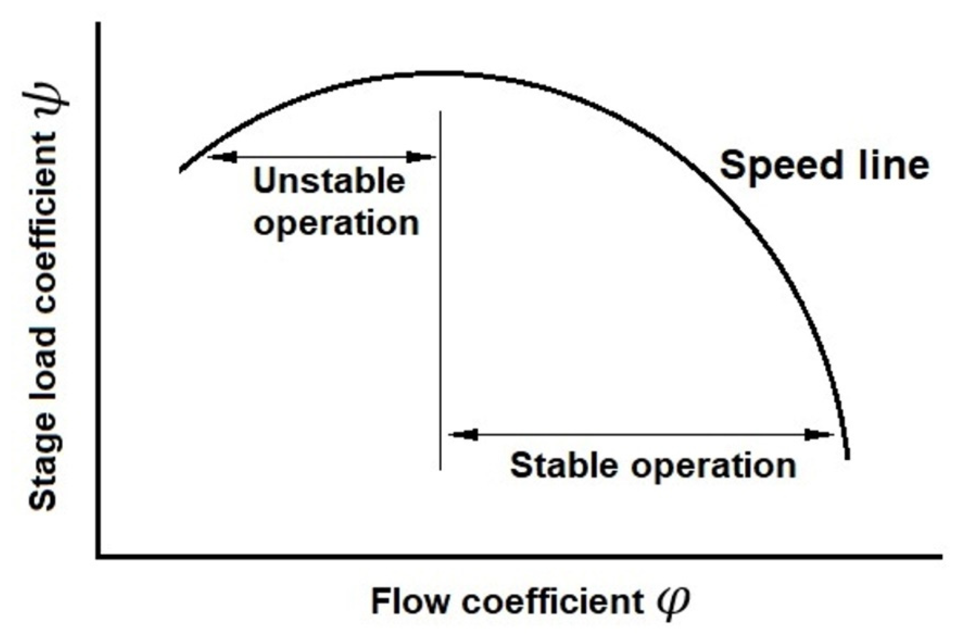
21] has been extended by considering HFDT data set at different rotational speeds and with an offset in IGV position outside of its scheduled nominal position with respect to GGS. The developed 1-D compressor modeling architecture is interfaced with a 0-D twin-shaft engine model in the Simulink environment to predict the dynamic inter-stage performance of the axial compressor during a step load change, air bleed off from the engine center-casing, and offset in IGV position outside of its scheduled nominal position with respect to GGS. It is possible to simulate the dynamic performance of a multistage axial compressor during a twin-shaft IGT operation and represent it in the overall compressor map and individual stage characteristic maps. The overall modeling framework is validated with real-world test data of a twin-shaft engine measured during the load acceptance tests. The representation of the dynamic compressor performance on stage-characteristic maps can provide valuable information during the dynamic operation of an axial compressor in the field. For example, during the dynamic transition between two operating conditions, a given stage may perform close to its stability limit, which could cause instability of the whole compressor during the dynamic operation, particularly at low speeds. Such instability in the compressor could compromise the performance and operability of the whole IGT.
This manuscript is organized as follows: A brief description of the 1-D compressor modeling architecture from a previous study [
21] is presented in
Section 2. HFDT data set at different rotational speeds and with the offset in IGV position outside of its scheduled nominal position with respect to GGS structure are presented as well. In
Section 3, a Simulink model of an IGT interfaced with the 1-D compressor model is presented. The dynamic validation of the modeling architecture with real-world data measured during load increase in an IGT is presented in
Section 4. The results are presented in
Section 5, which demonstrates the dynamic performance of the compressor represented in the overall compressor performance map and stage-performance maps. The manuscript is concluded with
Section 6, which summarizes the main results.
2. Compressor Modeling Architecture
In a previous study [
21], the 1-D model of the axial-compressor was developed. A brief summary of the devised model is described in this section. The inter-stage modeling framework considered theoretical velocity triangles, which relate the power input to the axial compressor stage. An analysis of these velocity triangles utilizing trigonometric relations and thermodynamic principles can derive the temperature and pressure rise across the compressor stages. The following equations comprise the overall modeling framework. The difference in total temperature between the outlet and inlet of the compressor stage is defined as:
where
, U is the blade velocity, r is the tip radius, and ω is the angular velocity; α
1,2 represents the angle of the air absolute velocity from the axial direction C
X entering and leaving the rotor,
,
is the airflow rate,
is the air density, and A is the annulus area. λ is the work-done factor and accounts for the reduction in work capacity across the compressor axial stage [
1].
The pressure ratio through the stage can be defined as:
where η is the stage efficiency, and T
in is the stage inlet total temperature. The derivation of Equations (1) and (2) and the relation between the velocity triangles and thermodynamic principles have been reported by Saravanamutto et al. [
24].
The 1-D inter-stage compressor model developed in the previous study [
21] is mainly comprised of Equations (1) and (2) and requires the rotational speed ω, flow rate
, efficiency η and ambient temperature T
amb and ambient pressure P
amb as inputs. The outputs from the 1-D compressor model are the pressure ratio P
R and temperature T
out across the different stages of the axial compressor. In addition, compressor design parameters and the Equations (1) and (2) were required to develop the semi-empirical 1-D modeling architecture. The annulus area A, tip radius r and blade angles across the different stages of the compressor were provided by a compressor manufacturer. Thermodynamic parameters represented in Equations (1) and (2) such as air density
, heat capacity C
P, and the ratio between heat capacities γ across the different stages are calculated through data representing stagewise temperature and pressure ratio collected from an HFDT. HFDT is a Siemens standard through flow analysis code that computes the performance of the multistage compressor as an axisymmetric model. HFDT is essentially a two-dimensional computational fluid dynamics code based on the streamline curvature method, as reported by Wu [
22]. For a given operating condition defined by the speed and throttle set by the compressor exit pressure, the code calculates the primary flow parameters such as pressure, the temperature at defined axial stations. Typically, these stations are located at the inlet and exit of the blade rows. The use of throughflow analysis for estimation of inter-stage pressure and temperature in a multistage axial compressor was reported in the study of Damiani et al. [
20]. Schnoes et al. [
25] considered throughflow analysis for the design optimization of a 15-stage axial compressor.
A constant efficiency η is considered in the calculation of pressure ratio across the stages (Equation (2)). The efficiency η is obtained from a 0-D model of compressor map (pressure ratio and speed as input and efficiency as output) related to the 11-stage axial compressor considered in this study. Schnoes et al. [
25] estimated the efficiency η across the stages of a 15-stage axial compressor using throughflow analysis and demonstrated a variation of the efficiency η across the different stages. In this study, a constant efficiency η is considered in the calculation of pressure ratio (Equation (2)). The parameter λ in Equation (2) accounts for the variation of efficiency η across the stages to match the pressure ratio estimated from HFDT and estimated by Equation (2).
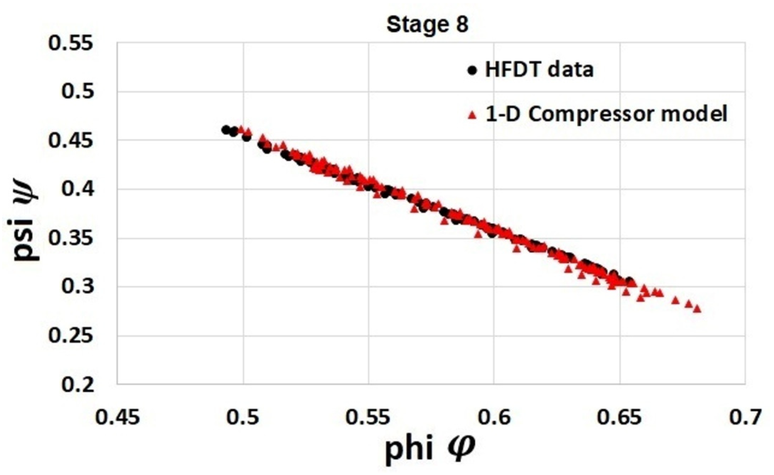
In this study, the pressure ratio for each stage has also been collected from the HFDT during compressor simulation at different rotational speeds and at a different offset in the IGV position. Stagewise pressure ratio collected from the HFDT allows the validation of the compressor model at steady-state conditions. This has been demonstrated in a previous study [
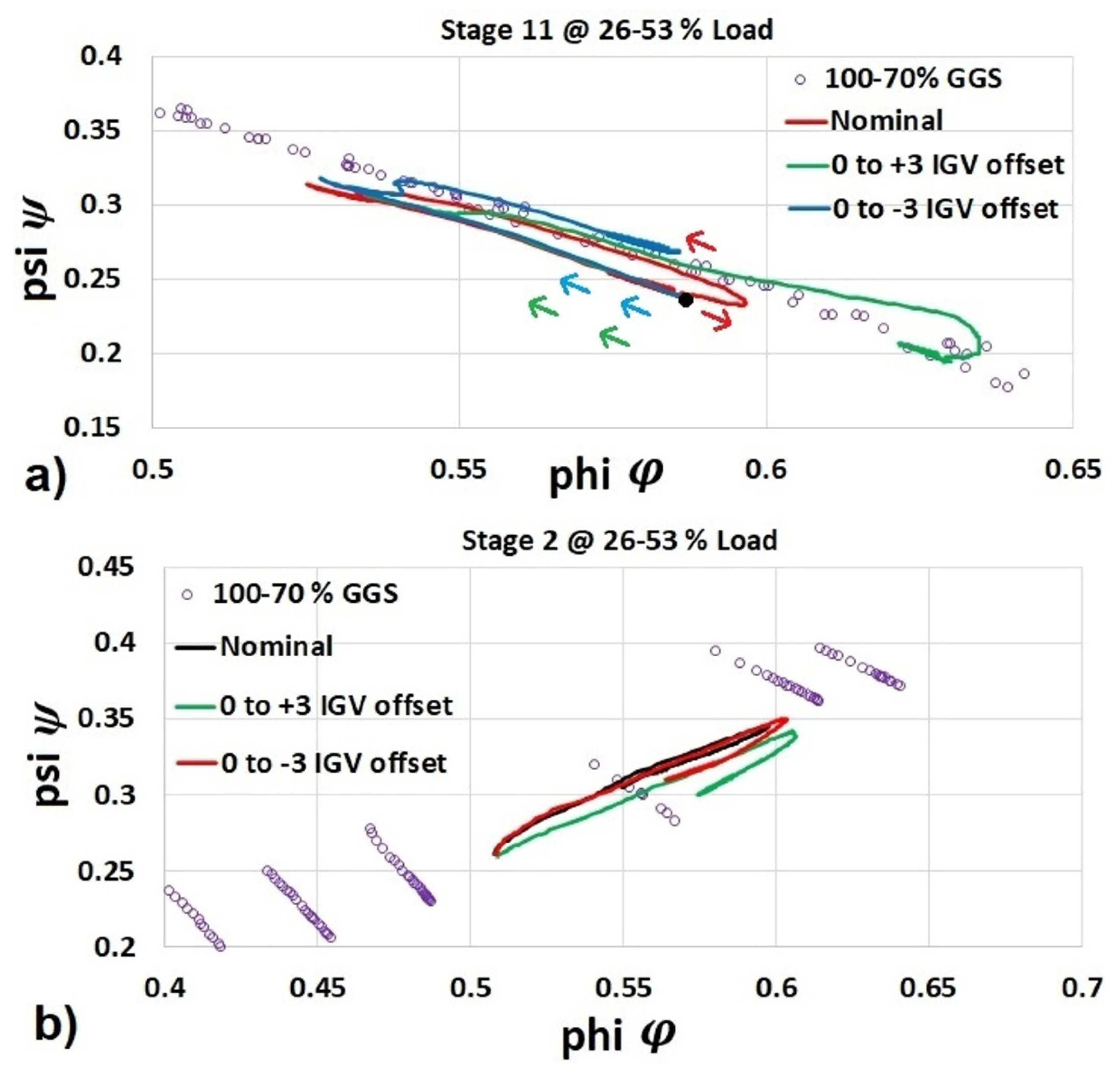
21]. The IGV demand angle was scheduled with respect to compressor speed. The position (in degrees) of VGVs is a function of IGV position. An offset in the IGV position is considered as a position of the IGV outside its scheduled position with respect to the GGS.
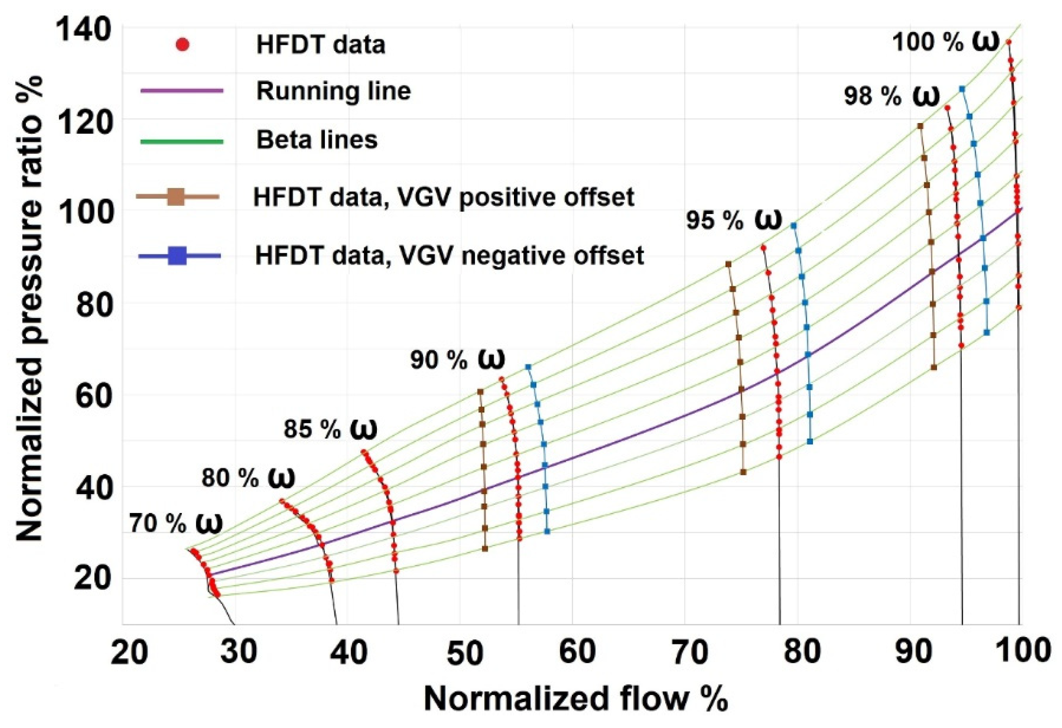
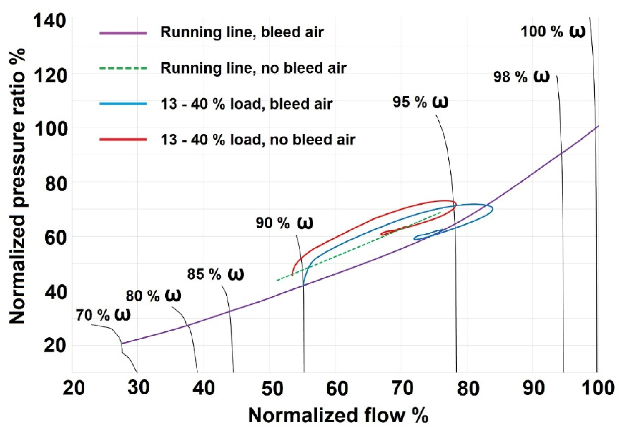
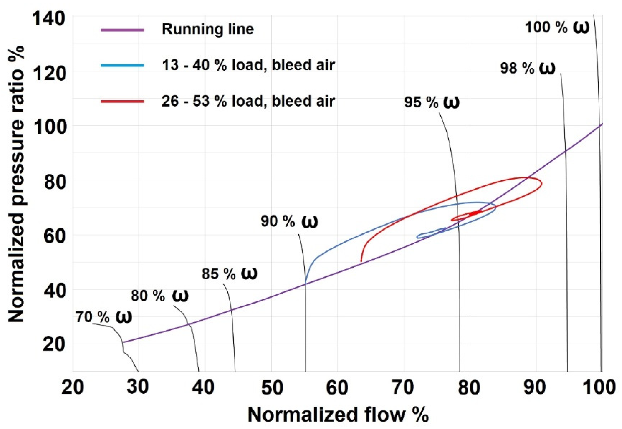
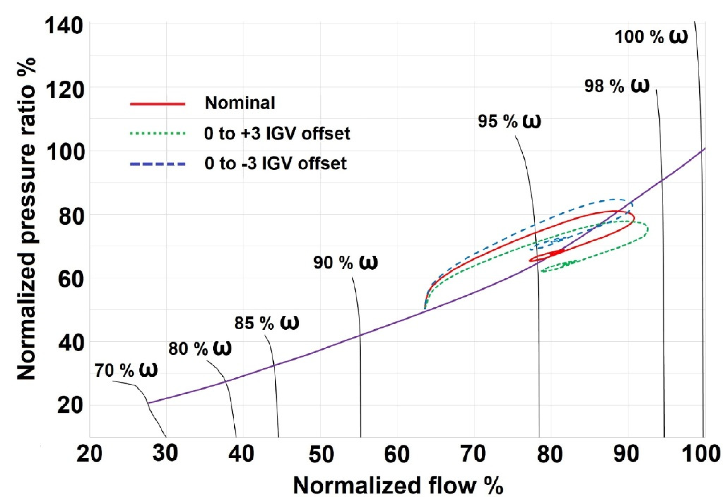
Figure 1 shows the total pressure ratio calculated by the HFDT and represented in the overall compressor performance map of an 11-stage axial compressor. The compressor map was validated with real-world compressor data. The total pressure ratio estimated from the HFDT is calculated by multiplying the individual pressure ratio across the stages comprising the 11-stage axial compressor. The compressor map shown in
Figure 1 considers 9 “beta lines” across each speed. These beta lines will allow the interpolation of pressure ratio between different speeds and flow rates during the dynamic compressor simulation. The running line representing the overall operating range of the compressor is shown in
Figure 1. It shows the total pressure ratio vs. flow rate at different operational speeds. The pressure ratio and flow rate were normalized with respect to the pressure ratio and flow rate values at 100% speed and at nominal conditions. The operational speed was normalized with respect to the maximum speed ω
max.
Figure 1 also shows the pressure ratio calculated by the HFDT and considering an offset in the position of the VGVs outside its nominal scheduled position with respect to GGS.
The 1-D modeling procedure can be executed in the Matlab
® environment. It consists of an optimization process to estimate the parameter λ and a calculation process to predict stagewise temperature and pressure ratio. More information about the optimization process and calculation process from the 1-D compressor modeling architecture can be found in the previous study [
21]. White et al. [
26] presented a flow diagram to depict the 1-D modeling architecture of a multistage axial compressor. Their modeling architecture considers subroutines and estimates the blade angles across the stages in the compressor to predict overall compressor performance maps. This is in contrast to this study in which the geometry of the 11-stage compressor was provided by the compressor manufacturer.
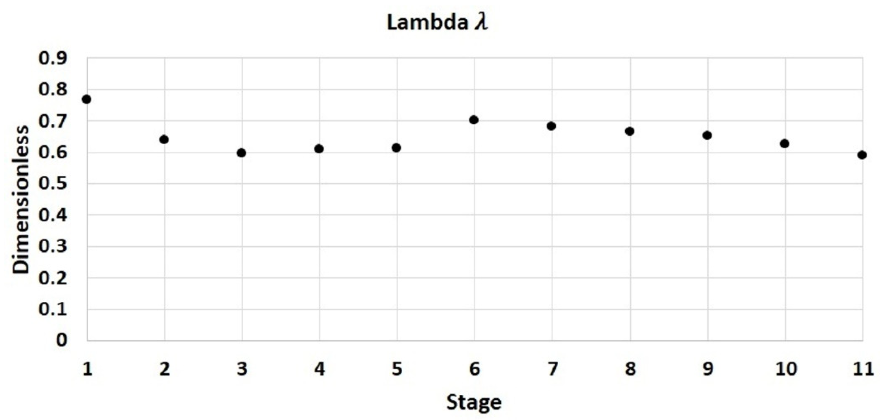
Figure 2 shows the estimation of the parameter λ related to the performance running line (
Figure 1) at 100% rotational speed and considering the optimization process from the 1-D compressor modeling architecture [
21].
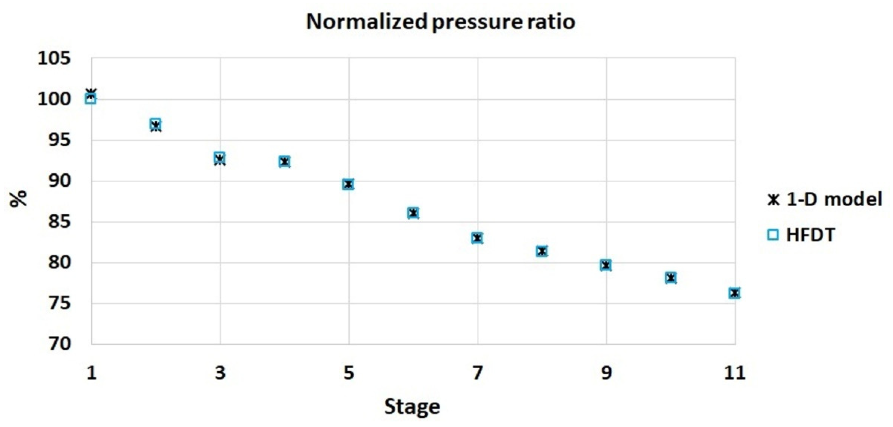
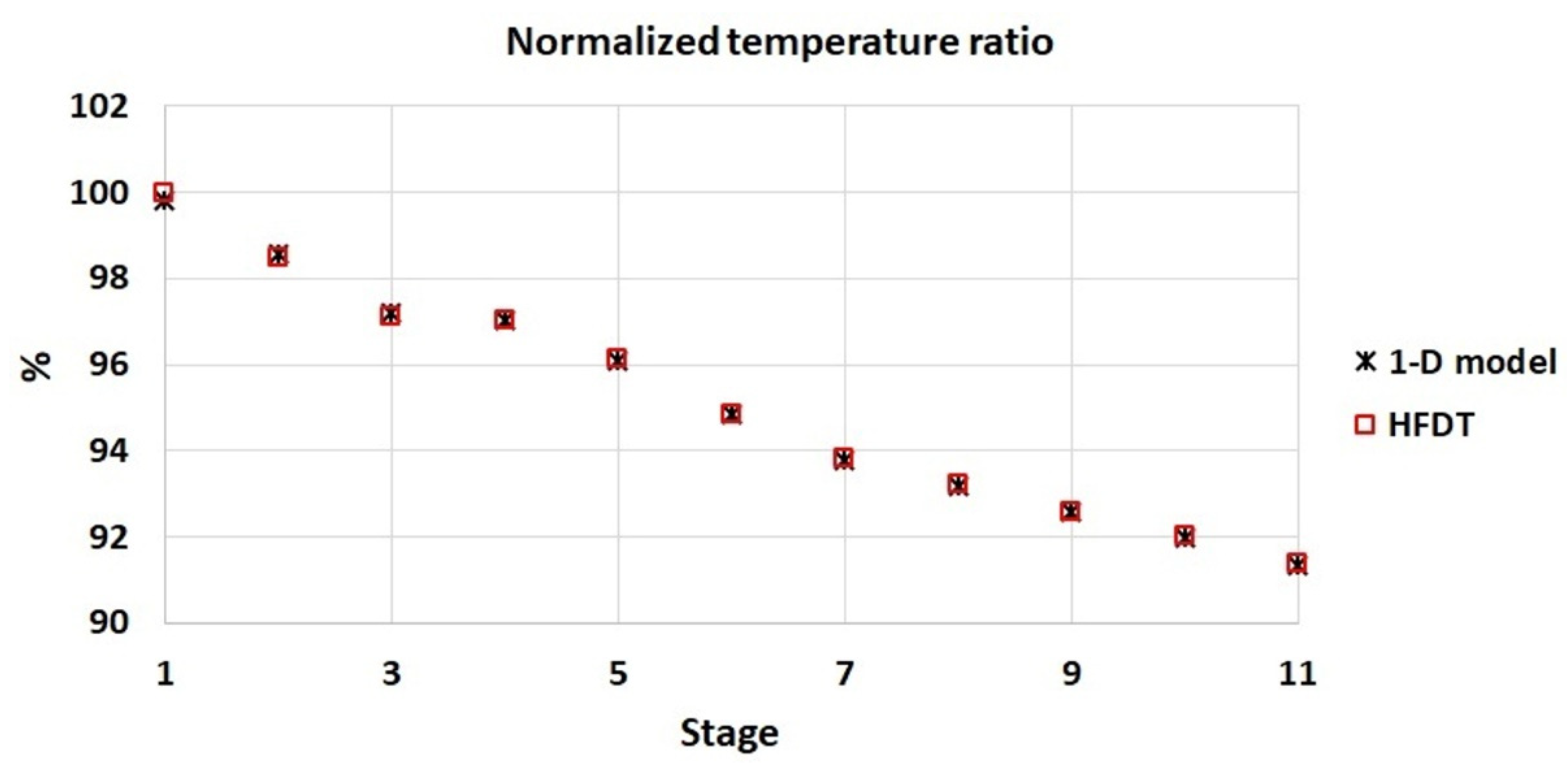
Figure 3 and
Figure 4 show the resulting stagewise pressure and temperature ratio calculated from the parameter λ and Equations (1) and (2) and considering the calculation process. The pressure and temperature ratio shown in
Figure 3 and
Figure 4 were normalized with respect to the maximum value of the HFDT stagewise data from the total pressure ratio of the compressor performance running line (design point) at 100% rotational speed.
3. Engine Modeling Architecture
A 0-D engine model constructed in a Simulink environment [
23] was considered for the simulation of the dynamic compressor performance of a twin-shaft IGT system at different load conditions.
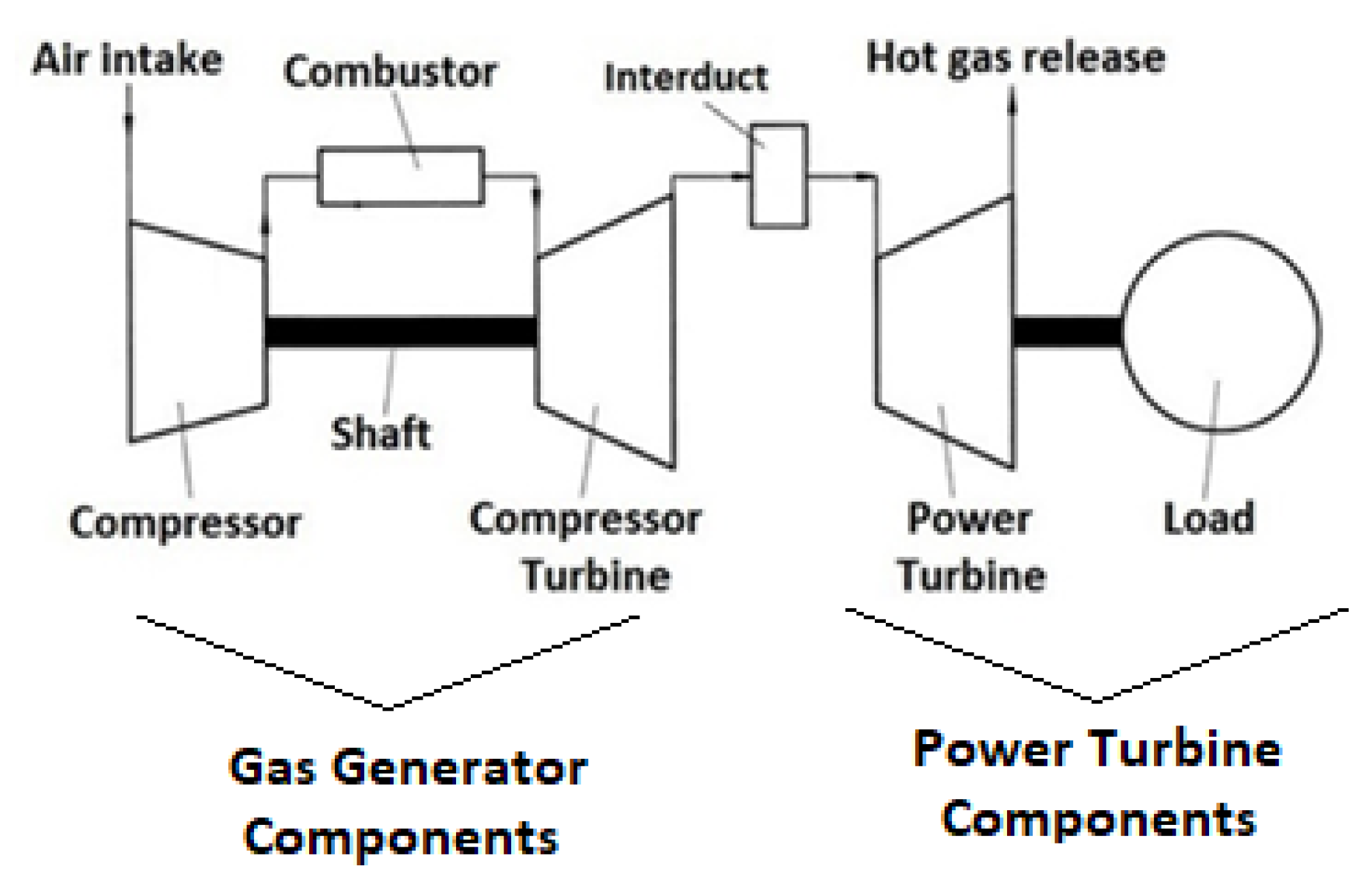
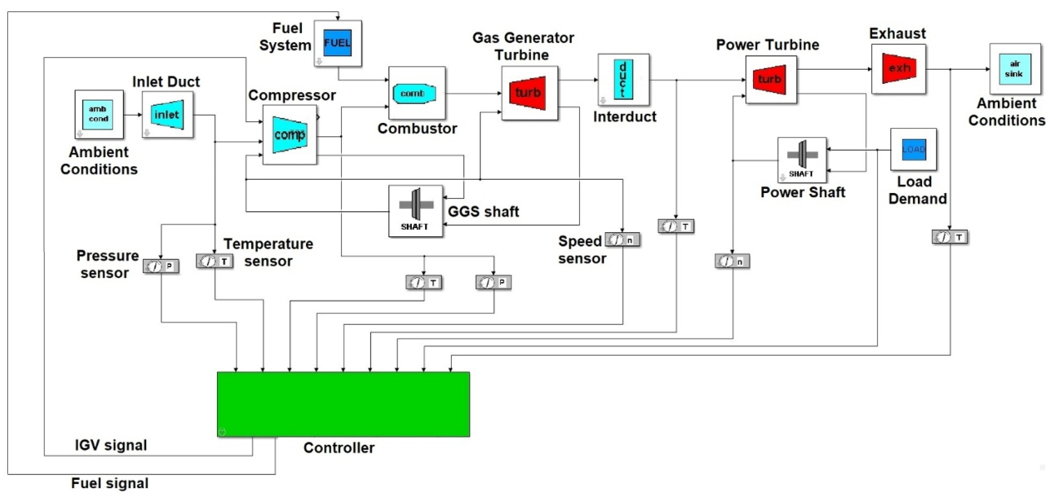
The 0-D twin-shaft engine model comprises gas generator components and power turbine components, and they are connected through an interduct component. The gas generator components comprise the compressor, combustor, gas generator turbine (GGT), and a shaft connecting the compressor and GGT, as shown in
Figure 5. Power turbine components comprise the power-turbine (PT), load, and mechanical shaft connecting the PT and load. As inputs, the model requires the load and the temperature and pressure of the air entering the compressor. Conservation of mechanical energy for shafts, heat-soaking effects for metal parts, and conservation of thermodynamic energy are included in the component models. The dynamic model of the gas turbine engine can be expressed with a system of nonlinear differential equations. The following equation is considered to model the dynamic response of pressure in the individual model components:
where ςj is the internal thermodynamic state. The first term on the right-hand side of Equation (3) represents volume gas dynamics, and the second term on the right-hand side describes the behavior of components using nonlinear algebraic equations. More details of Equation (3) and the differential equations representing the dynamic model of the twin-shaft gas turbine were reported in the study of Panov [
23].
The 0-D modeling architecture comprises a lumped axial compressor model and considers compressor performance maps for flow and efficiency as a function of pressure ratio and rotational speed. The 0-D engine model can predict the total flow, efficiency, pressure and temperature of air discharged by the compressor at steady and transient conditions. The normalized compressor flow map defined in the 0-D compressor model is shown in
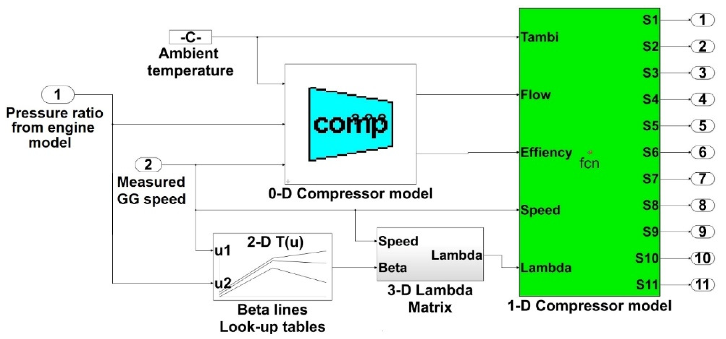
Figure 1. As discussed in the previous section, the 1-D model requires as inputs the temperature at ambient conditions, the airflow rate, efficiency, speed and lambda (λ work-done factor) values. The 0-D compressor developed in the Simulink environment [
23] is interfaced with the 1-D model, as shown in
Figure 6. The modeling architecture presented in this study combines the 1-D compressor model reported in a previous study [
21] and developed in the Matlab
® with the 0-D twin-shaft gas turbine model developed in the Simulink environment and reported by Panov [
23]. As shown in
Figure 6, both modeling architectures can be interfaced in the Simulink environment by feeding parameters from the 0-D twin-shaft engine model into the 1-D compressor model. The 1-D model requires flow, efficiency, and speed from the 0-D compressor (twin-shaft gas turbine model) and calculates the pressure and temperature rising across the different stages of the multistage axial compressor.
Values of the parameter λ are required in the 1-D compressor model, as discussed in the previous
Section 2. A 3-D matrix defined in the Simulink environment was defined to include all the values of the parameter λ. The 3-D matrix calculates 11 values for λ from a given speed, a given value of IGV offset and a defined point on the beta line from the compressor map shown in
Figure 1. The calculated vector of λ values is provided to the 1-D model to calculate stagewise pressure and temperature across the 11 stages of the compressor. The overall modeling architecture comprises the 0-D engine model and the 1-D compressor model, as shown in
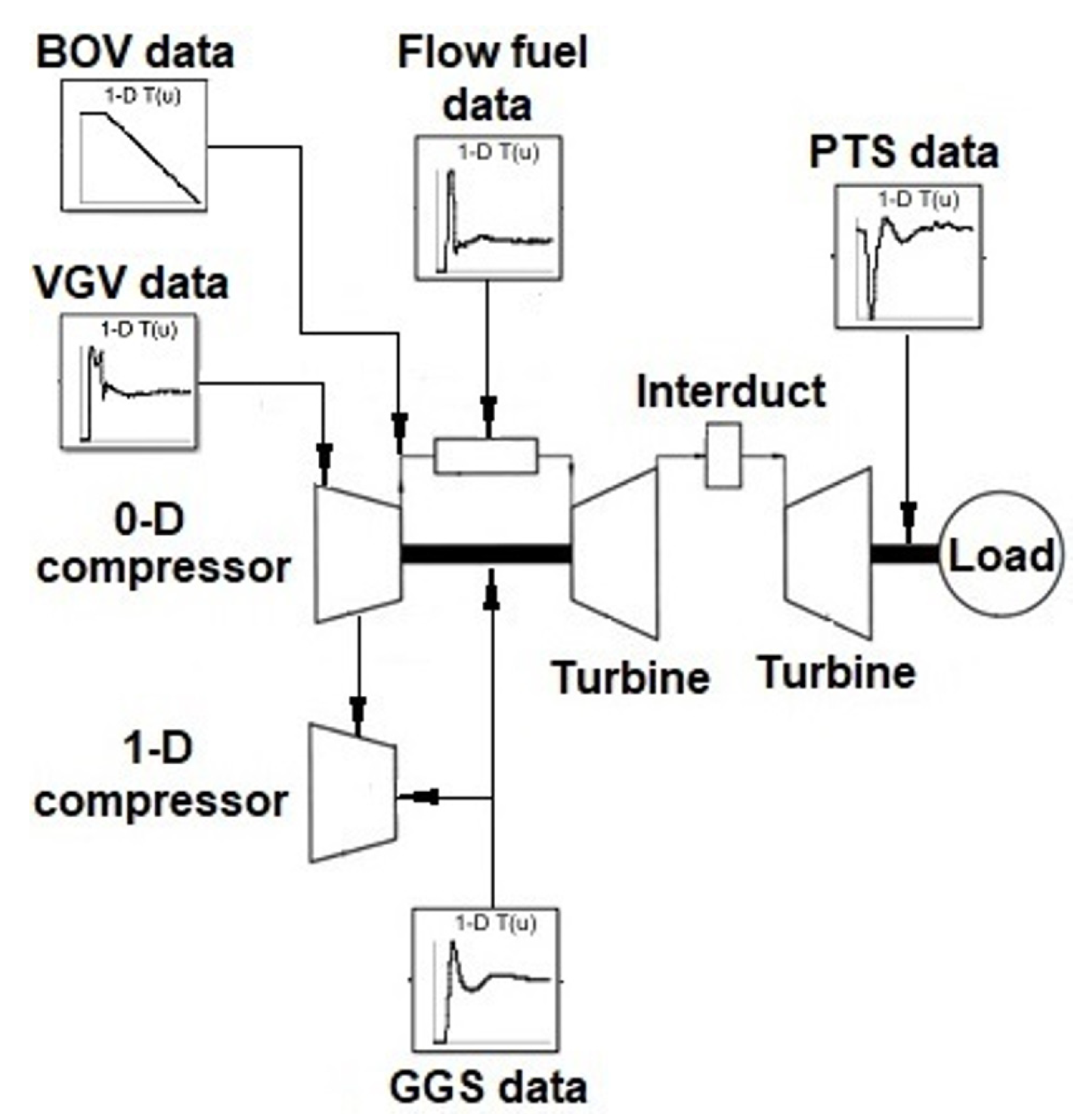
Figure 7.
The gas turbine data measured during the engine test of a twin-shaft IGT are provided to the different components of the 0-D engine model. The deployed gas turbine 0-D model does not contain a control system and mechanical system components such as the GG shaft and the PT shaft. Therefore, GGS, power turbine speed (PTS) and control system variables such as fuel flow demand (FFDEM), VGV demand (VGVDEM) and bleed\blow-off valve demand (BOVDEM) positions are provided to the 0-D gas turbine as a time history obtained from engine test. The engine model calculates the pressure ratio of the 0-D compressor model from the measured engine data and provides the flow to the 1-D compressor model. The 1-D model calculates the dynamic inter-stage compressor performance at different engine load conditions. This will be demonstrated in the results section.
4. Compressor Dynamic Validation
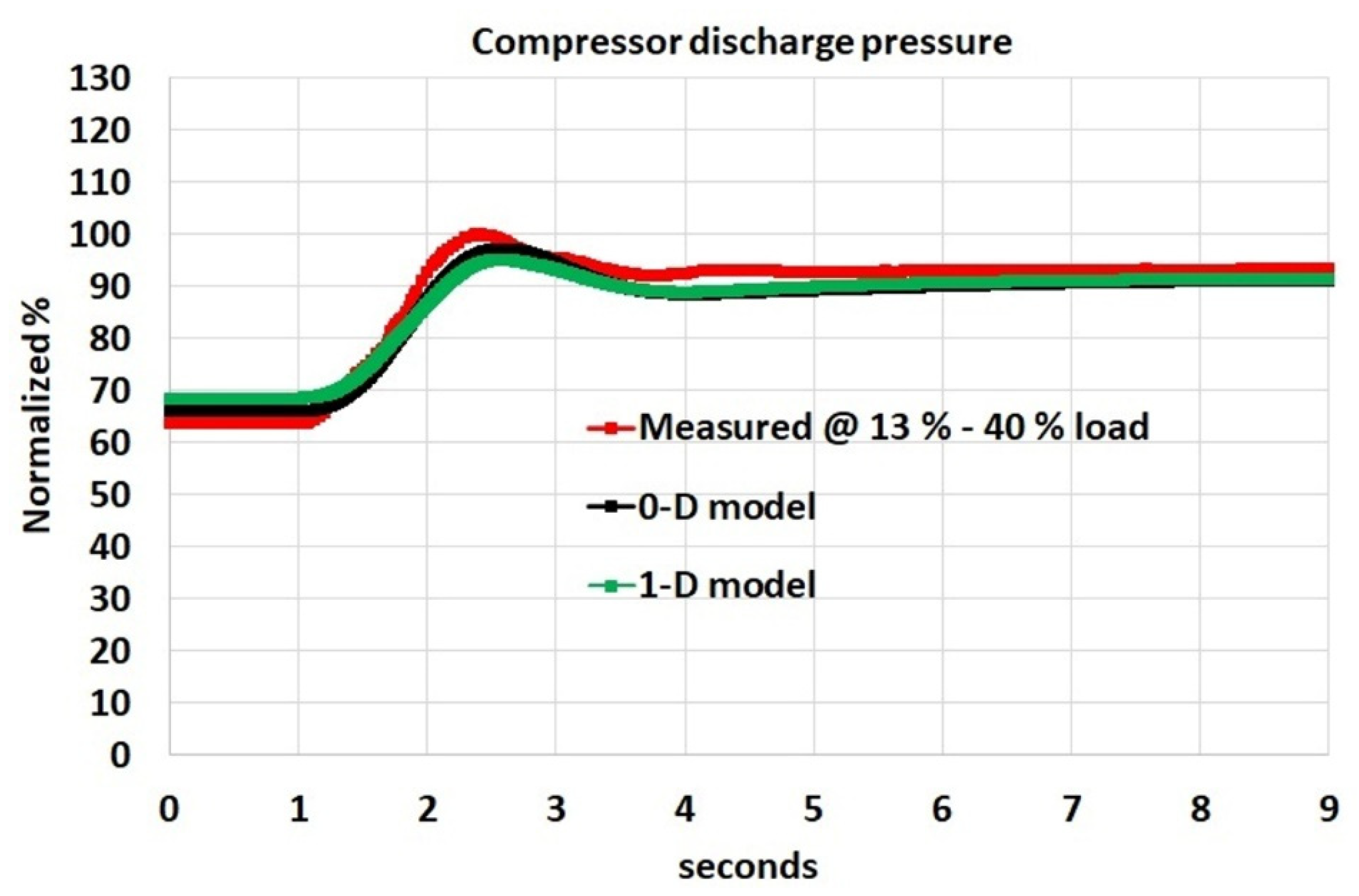
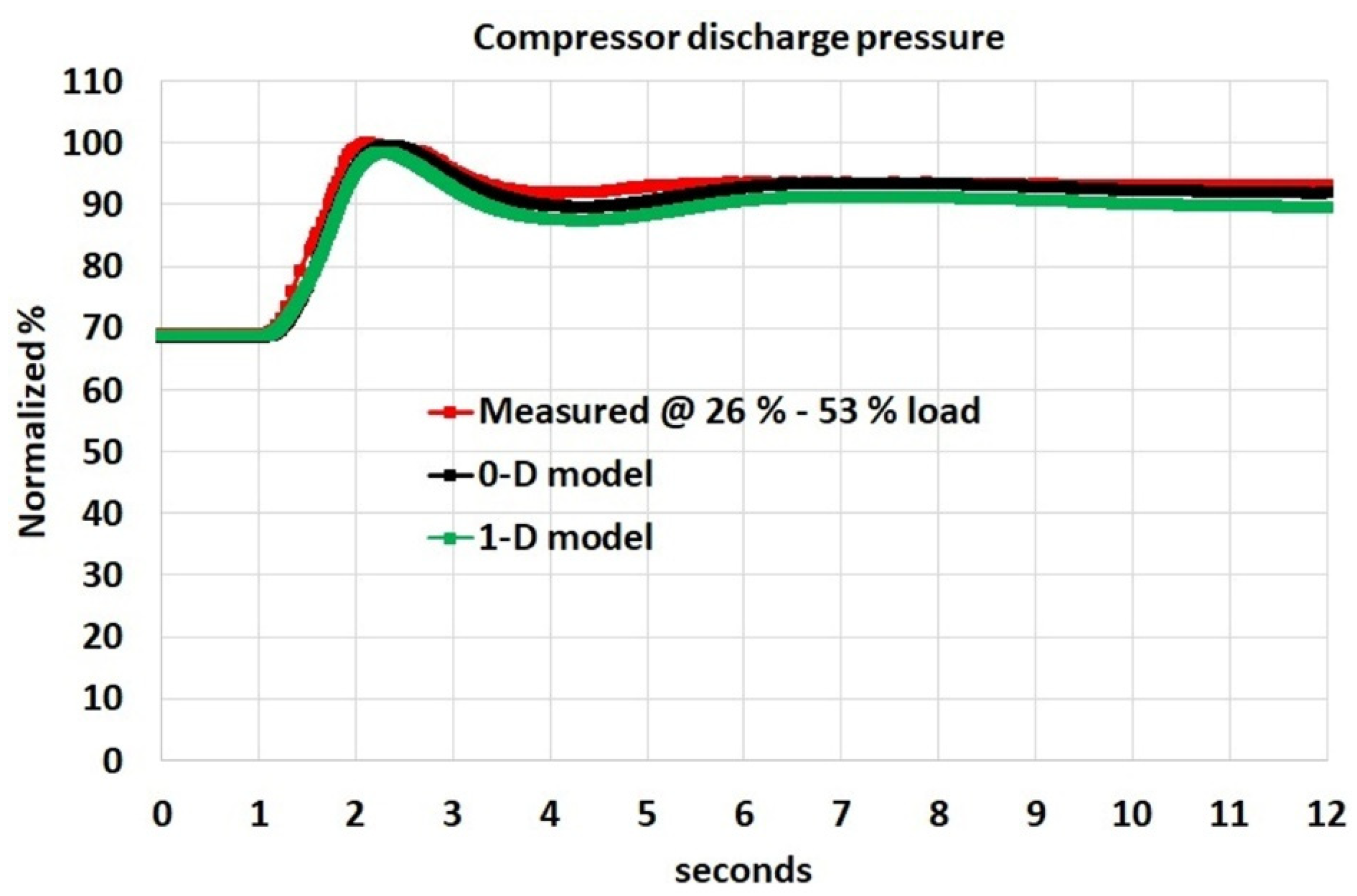
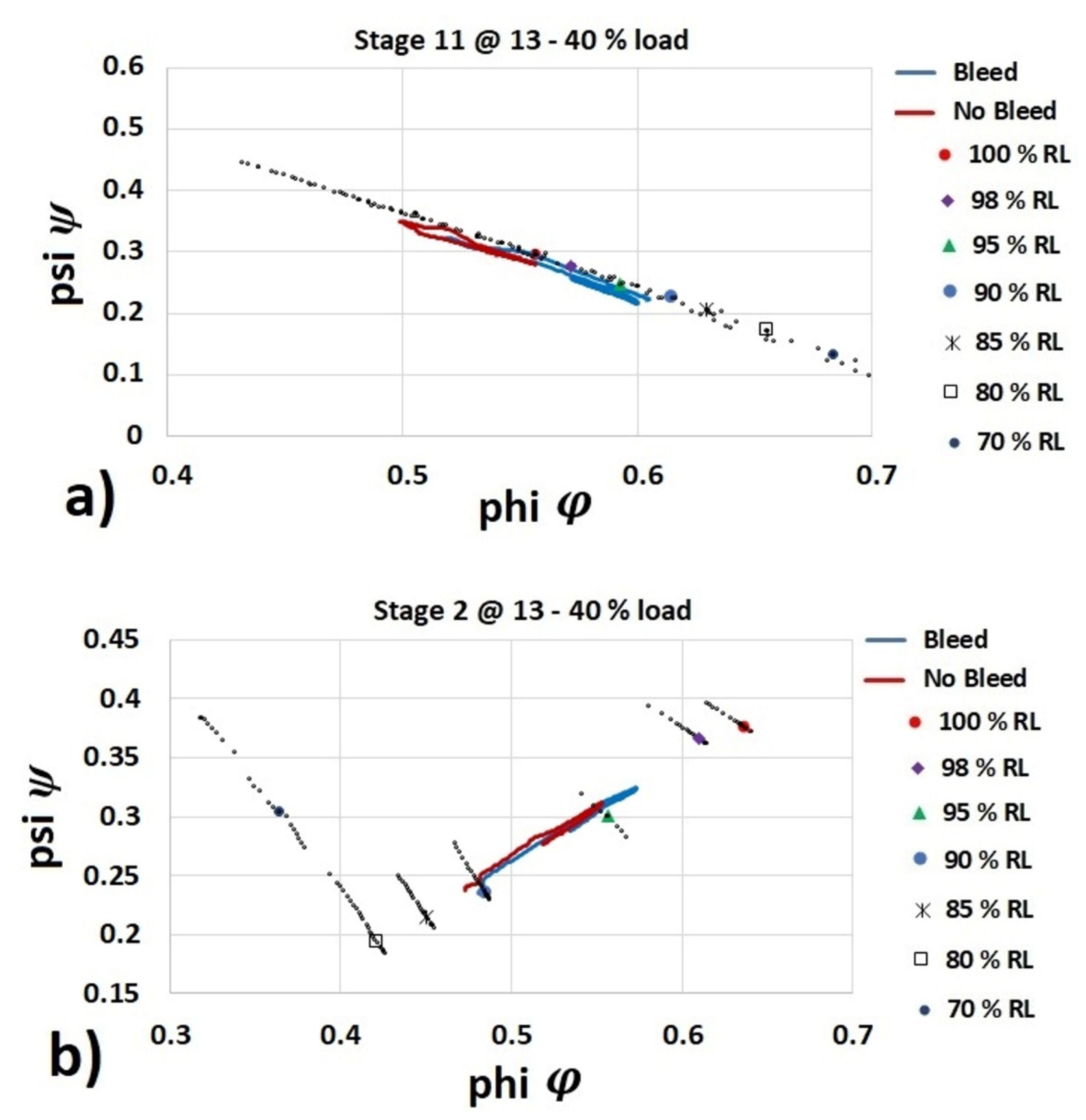
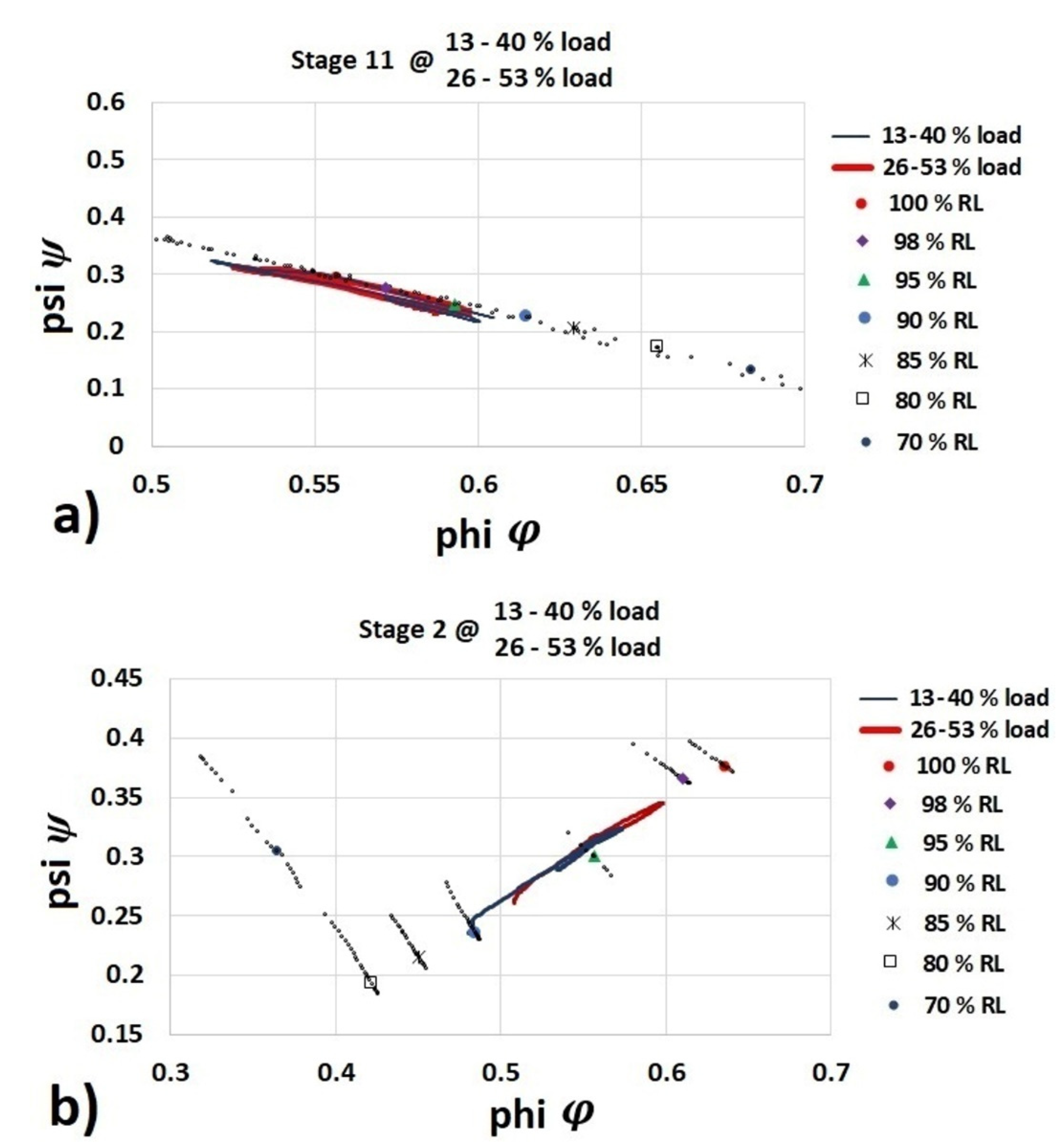
Measured engine data from a twin-shaft gas turbine operated during load acceptance test were considered for the validation of the developed model. The engine test data were logged during a step change in engine load from 13% to 40% of the maximum engine load. Two sets of measurements when increasing engine load from 13% to 40% were considered. The first set of measurements considers engine operation with air bleed from center-casing for the purpose of emission control–CO turndown. The second set of measurements was taken during engine operation without air bleed, which corresponds to natural turndown engine operation. In addition, measurements during engine tests with center-casing air bleed during load acceptance from 26% to 53% of the maximum load have also been considered.
The engine data comprise FFDEM, GGS, PTS, VGVDEM position, BOVDEM position and compressor discharge pressure (CDP). The FFDEM, BOVDEM, VGVDEM, GGS and PTS data are considered as inputs in the modeling architecture as shown in
Figure 7. The measured CDP allowed the validation of the compressor model.
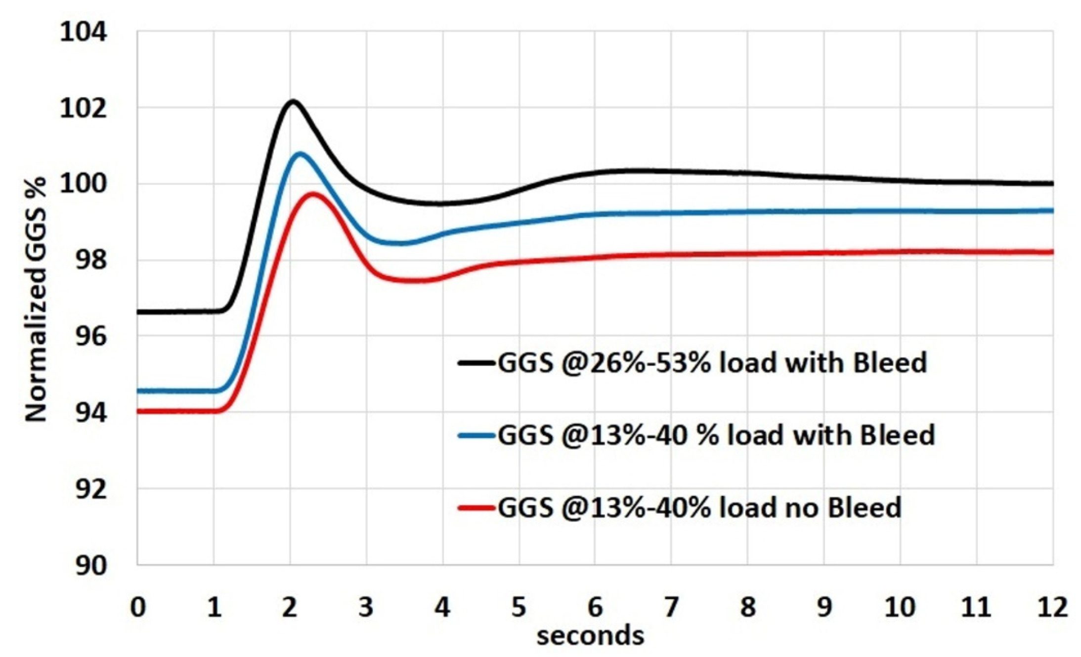
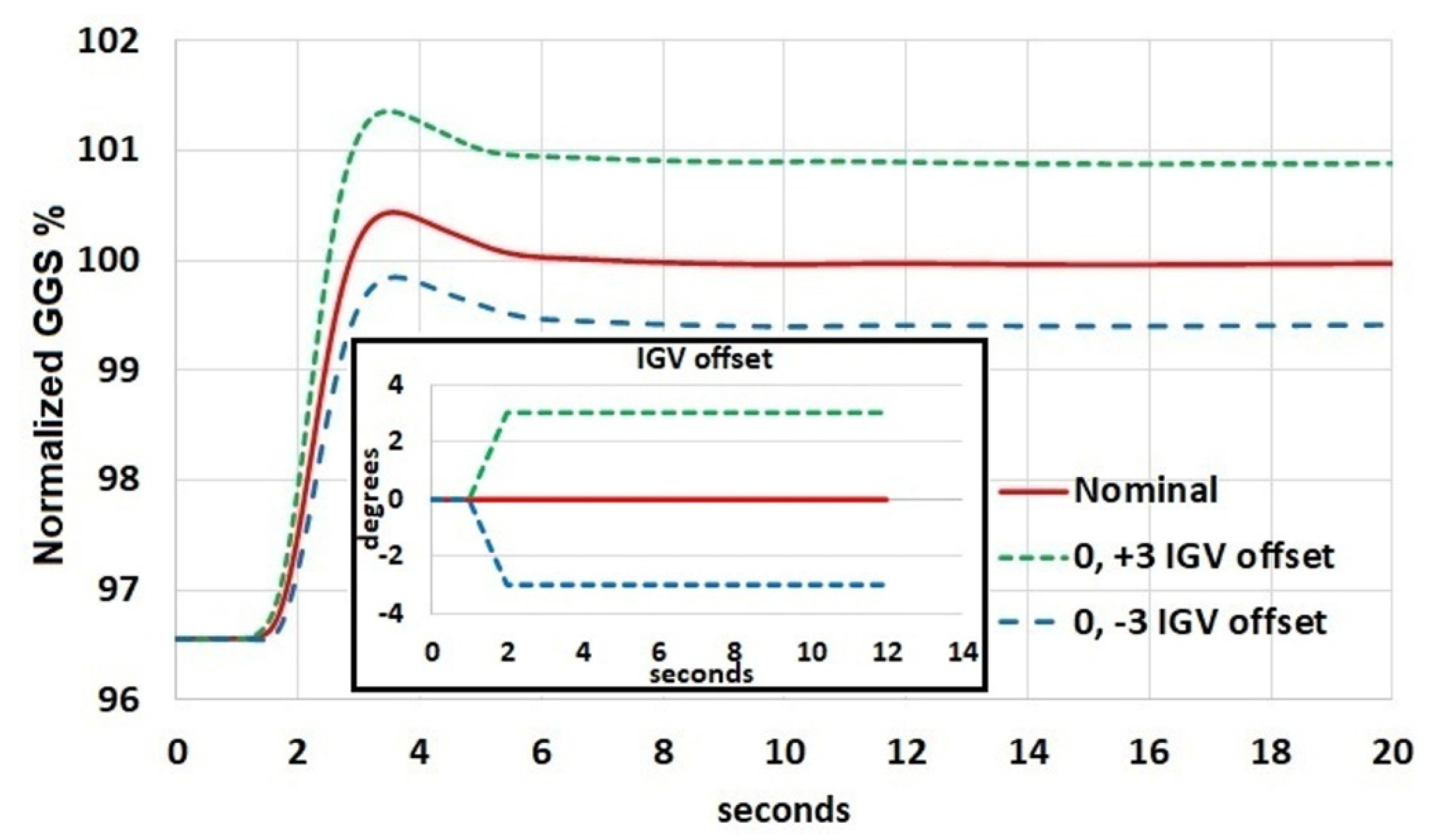
Figure 8 shows the normalized GGS with respect to the measured GGS at steady-state at 53% load. A decrease in measured GGS is observed when no air bled from center-casing is considered, and with increasing load demand from 13% to 40%.
Figure 9 and
Figure 10 show a comparison between the measured CDP and the predicted CDP from the 0-D and 1-D compressor models. The volume gas dynamic expressed in Equation (3) was considered in the 0-D compressor model to simulate the transient response of the CDP, as shown in
Figure 9 and
Figure 10. The interaction between the 0-D and 1-D compressor models is shown in
Figure 6. The 1-D compressor model requires as inputs the air mass flow and efficiency calculated by the 0-D compressor model and calculates the stagewise pressure ratio across the 11 stages. The total pressure ratio estimated by the 1-D model is calculated by multiplying all the individual stagewise pressure ratio across the 11 stages. In addition, pressure loss related to the compressor diffuser and outlet guide vanes was considered to approximate the simulated 1-D compressor model response with the measured data.
Table 1 shows the error between the 0-D compressor model and measured data. The error between the 1-D compressor model and measured data are also shown in
Table 1. The error in the 1-D compressor model is higher than the error in the 0-D compressor model. From
Figure 9 and
Figure 10, it can be observed that the biggest discrepancy between the measured data and the 1-D compressor model is during the dynamic response. This is considered to be due to the steady nature of losses predicted by HFDT steady-state calculations. The 1-D compressor model was developed from the HFDT tool, which represents the performance of the multiaxial compressor at steady-state conditions. The increase in error between the simulated data from the 1-D model and the measured data during transient engine performance is mainly attributed to the fact that the 1-D model cannot accurately predict the measured data at transient conditions. The 1-D model was developed using simulated data from the HFDT, as shown in
Figure 1. The HFDT data represent the performance of the compressor at steady-state conditions.
