Abstract
In this paper, the mechanical behavior of concrete twin-shaft mixers is analyzed in terms of power consumption and exchanged forces between the mixture and the mixing organs during the mixing cycle. The mixing cycle is divided into two macro phases, named transient and regime phase, where the behavior of the mixture is modeled in two different ways. A force estimation and power consumption prediction model are presented for both the studied phases and they are validated by experimental campaigns. From the application of this model to different machines and by varying different design parameters, the optimization of the power consumption of the concrete twin-shaft mixers is analyzed. Results of this work can be used to increase productivity and profitability of concrete mixers and reduce energy waste in the industries which involve mixing processes.
1. Introduction
Nowadays the environmental impact is an important industrial focus, therefore, companies producing machines must improve product quality and reduce energy waste at the same time. To remain competitive, this objective must necessarily be achieved using fewer resources, less time, less money and paying attention to energy consumption.
In this scenario, the development of smart and flexible models able to evaluate the influence of the project parameters on the consumed energy can be very useful in order to optimize the machine productivity reducing the absorbed energy.
The mixing process is very important in the alimentary, pharmaceutical, chemical, nuclear and materials industries which employ different types of mixers. There are many studies in the field of mixing machines involving computational fluid dynamics (CFD) analyses for many types of mixers, such as static mixers [1,2] passive mixers [3], dough kneaders [4], stirred tank reactors [5,6], and continuous mixers [7,8].
The investigation of the mixing in stirred tanks was performed in [9,10,11], considering a generalized Newtonian fluid and numerical simulations examined the mixing behavior with Newtonian and non-Newtonian fluids in simplified geometries of twin-screw mixers [12,13,14]. Moreover, the influence of the mixer geometry and operating conditions were studied [15].
This paper focuses on twin-shaft concrete mixers and the concrete mixing machine design and optimization, which are topics of great significance for achieving high-quality production standards with reduction of costs and waste. For this reason, scientific research is often focused on the mixing phases modeling [16,17,18,19], in order to study the influence of the various design and production parameters on the entire mixing process and to find the best way to improve the concrete quality [20,21,22,23,24,25,26] and reduce phenomena such as power consumption, wear [27,28,29,30] and friction among mixing components and mixtures [31] and to predict the useful life of the mechanical mixing organs [32,33].
Concrete mixers can work by exploiting different geometrical configurations based on the positions of the mixing shafts and on the machine kinematics [34].
In this paper, the study and optimization of a twin-shaft horizontal mixer are presented and discussed. The aim of the paper is to present a model to study the mechanical behavior of twin-shaft mixers, based on the prediction of the exchanged forces between the mixture and the mixing organs and the power consumption when design parameters vary in a realistic production range. The presented model is based on the soil mechanics and foundations theory differently from the models proposed in the state of the art.
The evaluation of power consumption is done in the transient and regime phases of the mixing procedure, and the model is validated by means of experimental tests in a real production plant. Then it is applied to different machine models and sizes to define optimal design parameters.
The main studied design parameters influenced by the optimization process are the mixing blades and arms size and shape, the radius and length of the tank, the shaft spacing, the processed concrete volume, and the filling level.
2. Material and methods
2.1. The Mixing Cycle
The mixture presents different behaviors for the three general phases of a mixing cycle. The first stage, called dry phase, comprises three operations: The introduction of aggregates (sand and gravel) and cement and a dry premixing stage, without any water addition. In this phase, the resistance of the paste increases until the water is added to the mixture.
The second stage, called the wet phase, comprises two operations: The introduction of water and additives, which causes a change of the physical properties of the paste. In this phase, after a peak of resistance of the mixture, it starts to decrease, due to a lubricating action which arises when the cement paste starts to form. Tests on real mixing machines demonstrated that if water and sand are introduced contemporarily during the wet phase, the mixing forces are lower than when water and sand are added separately. This means that the dry material loading in the second case is the worst case in terms of forces but the mixing operation results to be improved [19].
The third stage is the final mixing phase, which starts after the water introduction and finishes before the discharge operation. In this phase, the complete homogenization of the paste is reached, and the resistance tends to have a constant trend (regime phase). The last phase of the mixing cycle is the discharge operation when the mixer’s tank is emptied, and a new mixing cycle can start.
The changes in the concrete behavior during the entire mixing cycle result in different modeling criteria both of the paste behavior and of the mechanical interactions between the mixture and the mixer’s components like blades and arms.
Considering that, in the wet phase the concrete behavior cannot be modeled in a univocal way and the mixing cycle can be ideally divided into two macro phases: The transient phase, comprising all the stages until the resistance of the paste tends to have a constant value and the regime phase, starting when the resistance becomes quite constant and finishing before the discharge operation.
A typical power consumption curve for a generic mixing procedure is represented in Figure 1. In this picture, label 1 represents the end of the first mixing stage, label 2 the end of the second mixing phase and 3 the end of the third mixing stage and the beginning of the discharge operation. From Figure 1 it can be observed that the power consumption is maximum in stage 2. In particular, the peak power can be found in the time period during the water introduction.
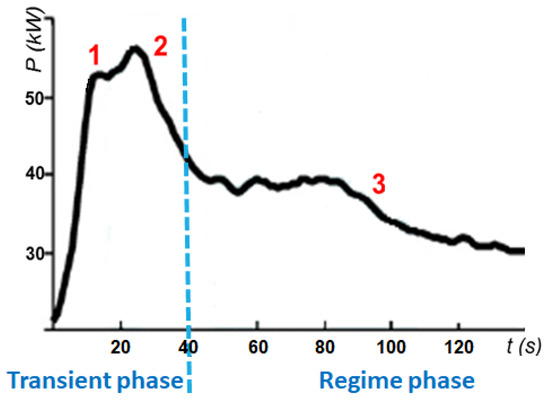
Figure 1.
Power absorption curve for a generic mixing cycle.
The blue dashed line in Figure 1 divides the two studied macro phases of the mixing cycle, previously defined.
2.2. Twin-Shaft Mixers and Geometrical Indices for Machine Comparison
Concrete twin-shaft mixers are horizontal mixers which work with a rotation of two horizontal mixing shafts (Figure 2). Typical components of these machines are the motors, one or more for each shaft, the gear boxes, the shafts, the tank and the mixing organs: Blades, arms, and connections.
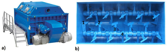
Figure 2.
Twin-shaft mixer and mixing components: (a) The machine, (b) the tank and mixing components: 1: Scraper, 2: Blade, 3: Arm and connection, 4: Shaft.
In the studied twin-shaft mixers, the tank has a typical omega shape, as represented in Figure 3, where some of the used geometrical parameters are shown:
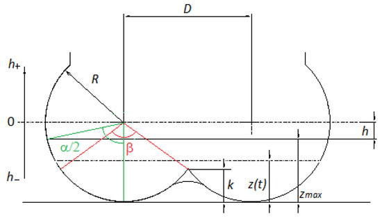
Figure 3.
Omega tank and geometrical parameters.
h is the filling level (m);
R is the tank radius (m);
D is the center to center distance between the two circles of the omega (m);
k is the height of the intersection between the two circles (m);
zmax is the filling height (m);
z(t) is the filling height function (m), where t is the time (s);
α/2(t) is the semi-angle representing the filling height at a certain time t (rad);
β is the angle, representing the intersection height (rad).
Based on these parameters, in this paper some additional geometrical indices have been defined in order to establish a criterion to compare different mixing machines:
I denotes the work index and C represents the compactness of the machine. In the formula of the work index, V represents the total volume for unit of length of the mixture and Vwork is the volume for unit of length processed at the same time by the two shafts of the mixer during the mixing cycle, which in turn corresponds to the volume for unit of length comprised between the intersection of the two circles of the tank and the filling level h (Figure 3).
The work index I can be considered as a representation of the machine productivity. The compactness index ranges from 0.5 to 1, as the ratio D/R ranges from 1 to 2. This means that the value of C increases with the compactness of the machine.
It can be observed that I and C increase accordingly, thus more compact machines can process bigger work volumes. Figure 4 represents the relationship between I and C.
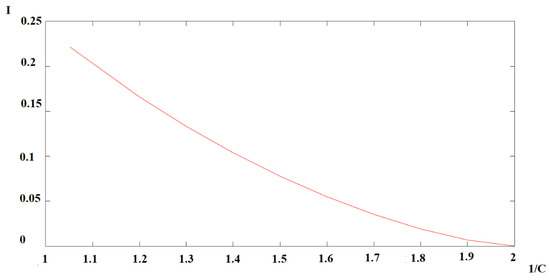
Figure 4.
Relationship between work index (I) and compactness of the machine (C).
3. Power Consumption Prediction Model
The developed power consumption theoretical model is mainly based on the calculation of the forces exchanged between the arm-blade assemblies and the mixture, during the transient and regime phases. These forces will depend on the rotating position of the arm-blade assembly and on the material filling level. From the knowledge of the forces, the power absorption is deduced and compared with experimental data from test campaigns performed using specific twin mixer models. As the mixture behavior can be modeled in different ways in the transient and regime phases, the model will be different for the two considered mixing stages.
3.1. Transient Phase
The power absorption in the transient phase will be calculated considering the model of the dry phase and predicting values very close to the peak, which occurs in the wet phase, where the mixture cannot be modeled in a univocal way.
In this stage, the mixture can be modeled as a granular material and treated by employing the Terzaghi’s mechanics of foundations theory [35,36]. According to this theory, the specific limit load qd (N/m2), reachable by a foundation without soil instabilities can be calculated as the sum of three contributions represented by forces due to the weight of the soil, forces due to the material cohesion and forces due to the material internal friction. For this reason, the specific limit load can be expressed by:
where c (N/m2) is the material specific cohesion, Nc, Nq, Nγ (dimensionless) are the load capacity factors as tabulated in [35], Df,i, (m) is the immersed quote of the ith component of the arm-blade assembly (Figure 5), which can be treated as a foundation, B (m) is a shape factor representing the width of the considered immersed part, γ (N/m3) is the material specific weight expressed as a load on the arm-blade assembly.
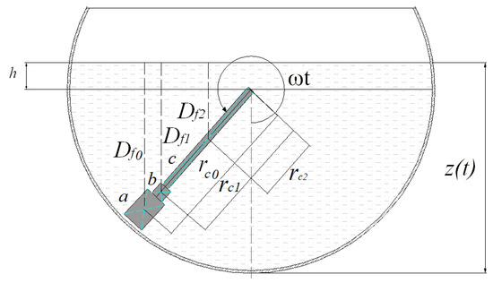
Figure 5.
Arm-blade assembly and immersed parts.
The load capacity factors depend on internal friction. The value of the internal friction angle considered in this model was 0.61 rad (35 degrees), as it results for the gravel sand in its loose state [19,35].
Considering Figure 5, the arm-blade assembly can be considered subdivided into three parts: The blade (a), the connection with the arm (b) and the mixing arm (c).
The immersed quote of the ith component of the arm-blade assemblies depends on time and can be calculated as:
where ω (rad/s) is the shaft angular speed and rci (m) are the distances of the center of gravity of the single ith components of the arm-blade assembly from the shaft, as represented in Figure 5 (i = 0 is the blade a, i = 1 is the connection b, i = 2 is the arm c).
From the calculation of the specific limit load, the total force acting on the arm-blade assembly can be calculated as the sum of all the three forces acting on the centers of gravity of the three components: Blade, connection, and arm.
The force on the single component can be expressed by:
where L(m) and B(m) are the length and width of the considered part respectively. cred,i(t) is a reduction coefficient which takes into account that the immersion of the ith component of the arm-blade assembly varies over time.
where is the radial length of the i-th component of the arm-blade assembly.
The calculation of the peak power absorption Ppeak(t) (W) is done considering all the contributions of the arm-blade assembly components:
The dependence on the time is necessary as the angular position, and the immersion quote of each arm-blade assembly are different at each instant.
The no-load power consumption was calculated by taking into account the inertia of the arm-blade assemblies and their number. Both the calculated peak power and no-load power were used to validate the model by comparison with the experimental measures.
The total peak absorbed power is:
3.2. Regime Phase
During the regime phase, the paste behaves as a viscoplastic material called Bingham fluid. This means that the mixture can be assimilated to a rigid body when subjected to low stresses and to a fluid when subjected to high stresses. Thus, the behavior of the paste can be described when the shear yield stress τ0 (Pa) and the plastic viscosity µ (Pa s/m) are known.
The law describing the stress τ (Pa) as a function of the velocity v (m/s) for a Bingham fluid is the following:
During this mixing phase, the force Fτ exchanged between the paste and the blades can be modeled as the force necessary to detach the mixture from the tank’s wall. For this purpose, the area AS (m2) of the wet surface of the tank must be calculated as:
where Lm (m) is the length of the mixer and () is the angle representing the area of the tank’s wall covered by the mixture (Figure 3).
Thus,
The regime power absorption Pregime (t) (W) results:
The calculated regime power was used to validate the model by comparison with the experimental measures.
The total regime absorbed power is:
4. Experimental Campaigns and Model Validation
4.1. Model Validation
The comparison between the theoretical and the experimental power absorption, is presented in Figure 6, where the only significant difference between the theoretical model and the experiment is noticeable in the early stages of material loading, as visible in the zoomed red box of Figure 6) [19].
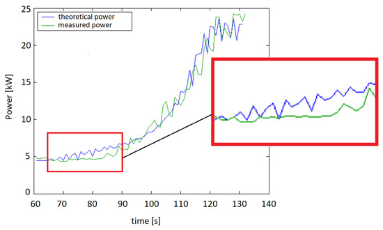
Figure 6.
Comparison between theoretical and measured power.
4.2. Experimental Campaigns
Four experimental campaigns were carried out to validate the model on the basis of the comparison between calculated and measured values of the peak, regime, and no-load powers.
An experimental campaign was carried out on a mixer model named “Model 1”, which processes 4.5 m3 of mixture and returns 3 m3 of vibrated concrete. “Model 1” has two motors with a nominal installed power of 55 kW for each motor. The geometrical parameters of the mixer used for the experimental campaigns are shown in Table 1.

Table 1.
Main geometrical parameters of the experimental mixer.
The experimental campaigns were performed by using a concrete composition with the same characteristics of the recipe used for the calculations, with cohesion of 1300 N/m2, a shear yield stress of 600 Pa and a degree of humidity equal to 5%, which is coherent with the cohesion value.
The power consumption curve for a single motor of “Model 1” mixer, resulting from the experimental tests, is represented in Figure 7, where the mixing time was extended with respect to the typical working time of the machine and the installed nominal power (55 kW) is highlighted.
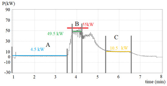
Figure 7.
Experimental power consumption curve for the single motor of “Model 1” with indication of power levels.
The value of regime power for the model validation was calculated as the average value of the measured powers in the area where the curve becomes flat before the discharge phase. The value of the peak power was calculated as the average value of the measured powers during the water introduction phase. In particular, one can observe the established bounds for the evaluation of the power consumption in the different phases by means of the gray vertical lines showed in Figure 7 and Figure 8.
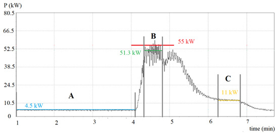
Figure 8.
Experimental power consumption curve for h = 0.344 m and one single motor.
The average values of the total peak power (49.5 kW), the total regime power (10.5 kW), the no-load power (4.5 kW) are highlighted according to the bounds indicated in the Figure 7 and Figure 8. Zone “A” represents the no-load power, zone “B” corresponds to the water introduction period used for the evaluation of the peak power, zone “C” represents the regime condition, when the power consumption reaches a quite constant value. The values of the power consumption obtained from the application of the power consumption prediction model, are reported in Table 2.
Table 2.
Analytical results of “Model 1” from the prediction model, considering both the motors of the machine.
As it can be observed, the experimental and calculated powers are completely superimposable, and the model results to be validated.
Other experimental campaigns were carried out with the same mixer and mixture composition, but with different filling levels h, so that the processed mixing volume changed. In particular, three different filling levels and mixing volumes were analyzed, as reported in Table 3, up to the working limit of the machine. Table 3 reports all the test and prediction results, which represent a further validation of the model.
Table 3.
Power results from the experimental test and for the prediction model, for different filling levels h, considering both the motors of the machine.
Figure 8 shows the experimental power consumption curve from the first test, where the mixing time was extended with respect to the typical working time of the machine.
5. Results and Discussion
Results of Table 3 show that using the same mixer and changing the filling level and the processed volume up to the technical limitations of the machine, the total regime power remains quite constant, while the total peak power presents a slight increase with h. Another aim of the paper was to study how the power consumption changed for different machine models and if the geometrical design parameters of a certain machine were changed of a certain amount. For this purpose, after the model validation, the prediction model was applied to another twin mixer model, named “Model 2”, which processes 3 m3 of mixture and returns 2 m3 of vibrated concrete. “Model 2” has two motors with a nominal installed power of 37 kW for each motor.
The two mixing machines “Model 1” and “Model 2”, were compared, and Table 4 reports all the calculated data of power consumption for the two studied machines and mixing phases. The power consumption was evaluated also considering some geometrical changes of the mixers, in order to assess what design parameters could be tuned to reduce the power consumption, especially in the transient phase. Small changes of radius and length of the machines (in the order of 1%) were considered to avoid changes in the number of arm-blade assemblies mounted on the mixer’s shafts and thus to perform a consistent comparison. In the comparison, both the shaft spacing distance D and the processed volumes were considered fixed.
Table 4.
Results of the prediction model with different geometrical parameters.
From these results it is clear that in the regime phase the power absorption increases both if the machine is lengthened and widened, leaving the shaft spacing distance as constant. This result is in agreement with the model formulas, as the regime power depends on the wet surface extent. One can observe that for both the machines and for a certain percentage of variation of R and Lm the regime power consumption is higher if the variation occurs for the radius. Using the compactness index already described, the results demonstrate that the absorbed power during the regime phase increases with compactness C, as it can be observed in Figure 9.
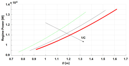
Figure 9.
Regime power vs. shaft spacing distance (D) and index of compactness (C).
In the transient phase, both the increase of radius and length cause a reduction of the filling level h. If the filling level decreases, also the immersion quotes of all the components of the arm-blade assemblies decrease and this results in a reduction of the total peak power. Furthermore, as a result, an increase of radius is better than an increase of length, as it causes a higher decrease of the peak power. This result was obtained without any measurement of the mixture homogeneity, which is neglected in this study.
Nevertheless, the results from Table 4 show that geometrical design parameters of the mixers need to be optimized with respect to the aim of the project. For instance, if the aim is an increase of processed volume and the transient phase is particularly critical for the power consumption, these results suggest the widening of the machine, according to the technical construction limitations.
Another application of the prediction model was performed to investigate how power consumption is affected by the blades’ shape. Two kinds of blades, normally used in the studied twin-shaft mixers, were considered: One with a “T” shape and one with an “L” shape, as represented in Figure 10. Results show that the total peak power is 9% higher for the T shape with respect to the L shape. Furthermore, the total regime power is 3.8% higher for the T shape with respect to the L shape. Thus, reductions of the power absorption can be obtained by using the blades with an L shape designed by the manufacturer of the studied mixers.
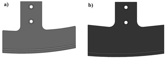
Figure 10.
Analysis of different blades’ shape: (a) L shape, (b) T shape.
6. Conclusions
The paper focuses on the concrete twin-shaft mixers and on a proposed mathematical model able to evaluate the power consumption as a function of the design parameters of the mixers. In this paper, the transient and regime phases of the mixing cycle were studied to calculate the forces exchanged between the concrete mixture and the mixing organs and the power consumption in twin-shaft mixers. For this purpose, a power absorption prediction model was presented, validated, and applied to different mixing machine models to investigate how to reduce the power consumption. Variations of design parameters such as the tank’s radius and length, the filling level, the processed volume, and the shape of the mixing blades were analyzed. Results show that increasing the filling level and the processed volume for a fixed tank’s geometry and number of arm-blade assemblies, the total regime power remains quite constant, while the total peak power presents a slight increase with h.
If the processed volume is kept fixed, in the regime phase the absorbed power increases with the index of compactness C and the work index I, defined in this paper and both with the tank’s radius and length. The increase with radius is higher than the increase with length. In the same conditions, the peak power registered in the transient phase decreases both when radius and length increase, but its reduction is higher when the radius is increased by the same percentage. This result was obtained without any measurement of the mixture homogeneity, which is neglected in this study. Results demonstrate also that if the mixer mounts the typical T blades, realized by the manufacturer, the total peak power is 9% higher than the case when the mixer mounts the L blades. In the regime phase, the total regime power with the T blades is 3.8% higher than the case with the L shape. Mixer’s manufacturers can benefit the results of this research for designing and producing machines which allow energy saving and enhanced production rates. In fact, the proposed model allows to study the machines with the aim of obtaining a greater production volume of concrete with the same installed power.
Author Contributions
Conceptualization, M.C.V., S.L., C.B., L.L.; data curation, M.C.V., S.L., L.G.; formal analysis, M.C.V., S.L.; funding acquisition, M.C.V.; methodology, M.C.V., S.L., C.B., L.L.; project administration, M.C.V., C.B., L.L.; software, M.C.V., L.L., S.L., C.B.; supervision, M.C.V., L.G.; validation, M.C.V., S.L., C.B., L.L.; writing—original draft, S.L., M.C.V.
Funding
This research received funding from Officine Meccaniche Galletti O.M.G. Srl, Perugia, Italy.
Conflicts of Interest
The authors declare no conflict of interest.
References
- Zalc, J.M.; Szalai, E.S.; Muzzio, F.J. Mixing dynamics in the SMX static mixer as a function of injection location and flow ratio. Polym. Eng. Sci. 2003, 43, 875–890. [Google Scholar] [CrossRef]
- Heniche, M.; Reeder, M.; Tanguy, P.; Fassano, J. Numerical investigation of blade shape in static mixing. AIChE J. 2005, 51, 44–58. [Google Scholar] [CrossRef]
- Tseng, L.; Yang, A.; Lee, C.; Hsieh, C. CFD-Based optimization of diamond-obstacles inserted micromixer with boundary protrusions. Eng. Appl. Comput. Fluid Mech. 2011, 5, 210–222. [Google Scholar] [CrossRef]
- Jongen, T. Characterization of batch mixers using numerical flow simulations. AIChE J. 2000, 46, 2140–2150. [Google Scholar] [CrossRef]
- Dhanasekharan, K.M.; Kokini, J.L. Design and scaling of wheat dough extrusion by numerical simulation of flow and heat transfer. J. Food Eng. 2003, 60, 421–430. [Google Scholar] [CrossRef]
- Wang, W.; Manas-Zloczower, I. Temporal distributions: The basis for the development of mixing indexes for scale-up of polymer processing equipment. Polym. Eng. Sci. 2001, 41, 1068–1077. [Google Scholar] [CrossRef]
- Lamberto, D.J.; Alvarez, M.; Muzzio, F.J. Experimental and computational investigation of the laminar flow structure in a stirred tank. Chem. Eng. Sci. 1999, 54, 919–942. [Google Scholar] [CrossRef]
- Alvarez, M.M.; Zalc, J.M.; Shinbrot, T.; Arratia, P.E.; Muzzio, F.J. Mechanisms of mixing and creation of structure in laminar stirred tanks. AIChE J. 2002, 8, 2135–2148. [Google Scholar] [CrossRef]
- Zalc, J.M.; Alvarez, M.M.; Muzzio, F.J.; Arik, B.E. Extensive validation of laminar flow in a stirred tank with three Rushton turbines. AIChE J. 2001, 47, 2144–2154. [Google Scholar] [CrossRef]
- Lamberto, D.J.; Alvarez, M.M.; Muzzio, F.J. Computational analysis of regular and chaotic mixing in a stirred tank reactor. Chem. Eng. Sci. 2001, 56, 4887–4899. [Google Scholar] [CrossRef]
- Connelly, R.K.; Kokini, J.L. Examination of the mixing ability of single and twin screw mixers using 2D finite element method simulation with particle tracking. J. Food Eng. 2007, 79, 956–969. [Google Scholar] [CrossRef]
- Connelly, R.K.; Kokini, J.L. 2-D numerical simulation of differential viscoelastic fluids in a single-screw continuous mixer: Application of viscoelastic FEM methods. Adv. Polym. Technol. 2003, 22, 22–41. [Google Scholar] [CrossRef]
- Kozic, M.S.; Ristic, S.S.; Linic, S.L.; Stetić-Kozic, S. Numerical analysis of rotational speed impact on mixing process in a horizontal twin-shaft paddle batch mixer with non-newtonian fluid. FME Trans. 2016, 44, 115–124. [Google Scholar] [CrossRef]
- Rivera, C.; Foucault, S.; Heniche, M.; Espinosa-Solares, T.; Tanguy, P.A. Mixing analysis in a coaxial mixer. Chem. Eng. Sci. 2006, 61, 2895–2907. [Google Scholar] [CrossRef]
- Rathod, M.L.; Kokini, J.L. Effect of mixer geometry and operating conditions on mixing efficiency of a non-Newtonian fluid in a twin screw mixer. J. Food Eng. 2013, 118, 256–265. [Google Scholar] [CrossRef]
- Cazacliu, B. In-mixer measurements for describing mixture evolution during concrete mixing. Chem. Eng. Res. Des. 2008, 86, 1423–1433. [Google Scholar] [CrossRef]
- Cazacliu, B.; Legrand, J. Characterization of the granular-to-fluid state process during mixing by power evolution in a planetary concrete mixer. Chem. Eng. Sci. 2008, 63, 4617–4630. [Google Scholar] [CrossRef]
- Cazacliu, B.; Roquet, N. Concrete mixing kinetics by means of power measurement. Cem. Concr. Res. 2009, 39, 182–194. [Google Scholar] [CrossRef]
- Braccesi, C.; Landi, L. An analytical model for force estimation on arms of concrete mixers. In Proceedings of the ASME Design Engineering Technical Conference, San Diego, CA, USA, 30 August–2 September 2009. [Google Scholar]
- Yao, Y.; Feng, Z.; Chen, S. Strength of concrete reinforced using double-blade mixer. Mag. Concr. Res. 2013, 65, 787–792. [Google Scholar] [CrossRef]
- Yao, Y.; Feng, Z.; Chen, S.; Li, B.Q.; Zhao, L.; Zhao, W. A Double-Blade Mixer for Concrete with Improved Mixing Quality. Arab. J. Sci. Eng. 2016, 41, 4809–4816. [Google Scholar] [CrossRef]
- Hu, C.; De Larrard, F. The rheology of fresh high-performance concrete. Cem. Concr. Res. 1996, 2, 283–294. [Google Scholar] [CrossRef]
- De Larrad, F.; Ferraris, C.F.; Sedran, T. Fresh concrete: A Herschel-Bulkley material. Mater. Struct. 1998, 31, 494–498. [Google Scholar] [CrossRef]
- Gram, A.; Silfwerbrand, J.; Lagerblad, B. Obtaining rheological parameters from flow test—Analytical, computational and lab test approach. Cem. Concr. Res. 2014, 63, 29–34. [Google Scholar] [CrossRef]
- Ferraris, C.F. Measurement of the rheological properties of high performance concrete: State of the art report. J. Res. Natl. Inst. Stand. Technol. 1999, 104, 461–478. [Google Scholar] [CrossRef]
- Marsili, R.; Moretti, M.; Rossi, G.; Speranzini, E. Image Analysis Technique for Material Behavior Evaluation in Civil Structures. Materials 2017, 10, 770. [Google Scholar]
- Valigi, M.C.; Logozzo, S.; Rinchi, M. Wear resistance of blades in planetary concrete mixers. Design of a new improved blade shape and 2D validation. Tribol. Int. 2016, 96, 191–201. [Google Scholar] [CrossRef]
- Valigi, M.C.; Logozzo, S.; Rinchi, M. Wear resistance of blades in planetary concrete mixers. Part II: 3D validation of a new mixing blade design and efficiency evaluation. Tribol. Int. 2016, 103, 37–44. [Google Scholar] [CrossRef]
- Valigi, M.C.; Fabi, L.; Gasperini, I. Wear resistance of new blade for planetary concrete mixer. In Proceedings of the 5th World Tribology Congress, WTC 2013, Torino, Italy, 8–13 September 2013. [Google Scholar]
- Valigi, M.C.; Logozzo, S.; Gasperini, I. Study of wear of planetary concrete mixer blades using a 3D optical scanner. In Proceedings of the International Mechanical Engineering Congress & Exposition, IMECE2015, Houston, TX, USA, 13–19 November 2015. [Google Scholar]
- Valigi, M.C.; Rinchi, M.; Caputo, S. Behavior Simulation of a Concrete Mix in a Turbine Pan Mixer. Available online: https://www.bft-international.com/en/artikel/bft_Behavior_simulation_of_a_concrete_mix_in_a_turbine_pan_mixer__2332434.html (accessed on 7 June 2019).
- Valigi, M.C.; Gasperini, I. Planetary vertical concrete mixers: Simulation and predicting useful life in steady states and in perturbed conditions. Simul. Model. Pract. Theory 2007, 15, 1211–1223. [Google Scholar] [CrossRef]
- Valigi, M.C.; Gasperini, I. Model-based method predicting useful life of concrete mixers [Modellgestütztes Verfahren zur Vorhersage der Nutzungsdauer von Betonmischern]. Betonw. Und Fert. -Tech./Concr. Plant Precast Technol. 2005, 71, 38–42. [Google Scholar]
- Ferraris, C.F. Concrete mixing methods and concrete mixers: State of art. J. Res. Natl. Inst. Stand. Technol. 2001, 106, 391–399. [Google Scholar] [CrossRef]
- Terzaghi, K.; Peck, R.B. Soil Mechanics in Engineering Practice, 3rd ed.; John Wiley and Sons Inc.: New York, NY, USA, 1996. [Google Scholar]
- Lancellotta, R.; Calavera, J. Fondazioni; Mc Graw Hill Education: New York, NY, USA, 1999; pp. 269–273. [Google Scholar]


© 2019 by the authors. Licensee MDPI, Basel, Switzerland. This article is an open access article distributed under the terms and conditions of the Creative Commons Attribution (CC BY) license (http://creativecommons.org/licenses/by/4.0/).