2.1. Design for Disassembly (DfD)
The disassembly of an object or a machine consists of the systematic disassembly of the various parts that compose it. The design for disassembly, more commonly known as DfD, is a design approach that allows easier recovery of parts, components, and materials that make up the product at the end of its life. DfD is therefore a design method that aims to improve quality and reduce time and costs related to disassembly of a product, considering waste and environment. Although DfD methods have existed for years, it is only in the last period that they have been applied more efficiently and consciously. This is due to the fact that over time, the market has accelerated its pace, proposing new goods in ever-shorter times and increasingly competitive prices (an example is the technological obsolescence of smartphones), in addition to the presence of directing pressures to the DfE, such as WEEE (waste electrical and electronic equipment), ELV (end of life vehicles) or RoHS (restriction of hazardous substances).
Disassembly plays an important role, as it can be performed for different purposes, such as performing preventive maintenance (replacement of a component that has not yet failed) rather than corrective maintenance (replacement or repair of a faulty component) or recycling the material of components that are no longer usable [
8].
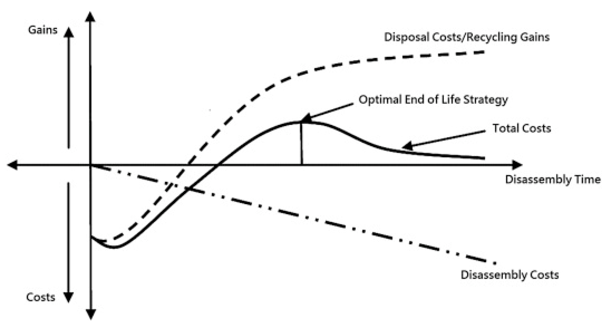
An essential aspect of DfD is calculating disassembly depth, i.e., the total number of sequential dismantling steps. In fact, it has been determined that the cost of dismantling is almost linear with the depth, while the revenue has a rapid initial increase and then settles down, without further growth as the depth increases. Using more time, energy, and resources in disassembling involves obtaining purer material, thus recovering part of the cost in terms of recycling and recovery. It is therefore a question of optimizing the area where there is more revenue for reasonable costs. For this reason, it is recommended in the DfD to place the most important components in easily accessible areas where possible (
Figure 1) [
9].
Among the advantages of the DfD, we therefore see a reduction in production costs, greater technical efficiency, greater flexibility during product development, and a reduction in resources.
2.1.1. Disassembly Sequence Planning (DSP)
Disassembly sequence planning, usually indicated with DSP, consists of the realization of a disassembly sequence coherent with the benefits that the DfD offers. The method is based on an efficient representation of the product and on the search for an effective sequence.
First of all, a disassembly can be of several types: We talk about complete disassembly when all the components are disassembled, while we have a selective disassembly when the product is not completely disassembled, but only until one or more specific components, called target components, are reached. Furthermore, we can have a nondestructive disassembly when the removal of the various parts does not entail rupture, thus allowing its revitalization and reuse. This disassembly, if it can be carried out, is generally preferable to destructive disassembling, which instead leads to the breaking of the components during disassembly. The DSP considers the product structure, the direction of removal of the components, the operational constraints, the complexity in representing the product, and the planning of the sequence. For this reason, there are guidelines that allow a sequence to be realized effectively and efficiently. First of all, the selection and use of materials and fasteners (connecting and/or fixing elements), component design, and product architecture must be considered.
To obtain a significant sequence, it is important to choose compatible recyclable materials, avoid using materials that require separation before disassembling, use components of the same type, and minimize and standardize the fasteners (for example using the same type of screw), thus making the components more easily separable and avoiding permanent fixings and toxic or dangerous materials. It is also important to remove the most relevant materials and components, to speed up operations by choosing between destructive and nondestructive methods, to move the product to be processed as little as possible, and to use electric or pneumatic tools, paying attention to the fatigue and effort of any person must support, as in the medium to long term, they can negatively affect their health and performance.
Below, we present two algorithms of DSP where it is useful to apply the DfD [
10].
2.1.2. 1st Method: “Research on the Selectable Disassembly Strategy of Mechanical Parts Based on the Generalized CAD Model”
This first method, introduced by Jianjun Yi, Bin Yu, Lei Du, Chenggang Li, and Diqing Hu, defines the order in which the components are removed to disassemble a selected component, called Cx. Once the Cx component has been defined, it is possible to identify all the possible sequences that allow the removal of our target component and, once identified, choose the sequence that best meets the objective function (for example, you can opt for the sequence with the minor number of operations to be performed, rather than the one that requires the least amount of time to be performed).
It is possible to define a generic Ci component in two different ways depending on the case series. A component Ci is defined as d-dependent when it is in contact with several elements that must be removed to allow disassembly of Ci, while 1-dependent is indicated as the case where it can be removed after removing only one component with which it is in contact.
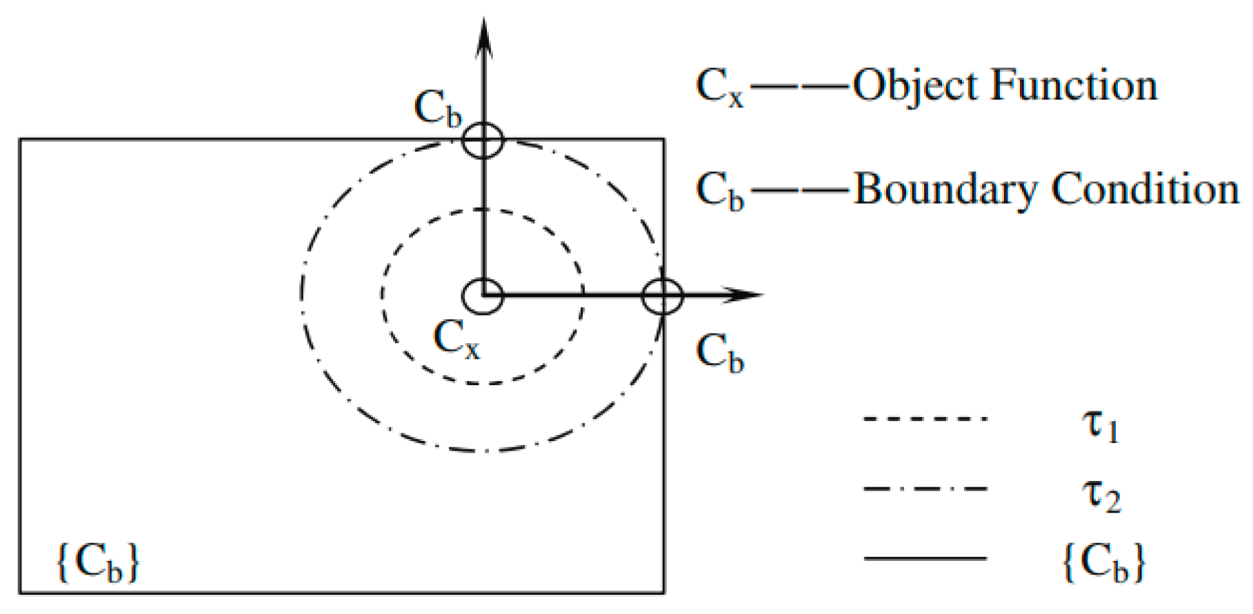
The identification of the various disassembling sequences was carried out through the use of the disassembly wave: We imagined that the Cx component is the origin of a wave that, starting at the time τ1, propagates in space, striking the elements in contact with the target component. Subsequently, a second wave, emitted at the instant τ2, touches the elements adjacent to the parts previously involved. This proceeds in an iterative way until all the elements have been involved, and we indicate with τn the generic instant in which the last wave is emitted. To then obtain the disassembly sequence (s), we began by removing the components present in the outermost disassembly wave (hence, the one corresponding to τn) and, proceeding backwards, we gradually removed the present components of the innermost wave disassembly, achievement of the Cx target component (the only component belonging to the instant τ0).
The whole is graphically represented by the removal influence graph (RG) (
Figure 2), in which the generic components C
i are represented with nodes, while it is indicated with the aid of arrows that the 1-dependent and d-dependent relationships connect the nodes, thus allowing to understand the dependencies between the components and providing a representation of the possible disassembly sequence (s). The disassembly wave instead is represented with a curve that connects all the nodes (i.e., the components) that are involved at the same instant τ
i generic.
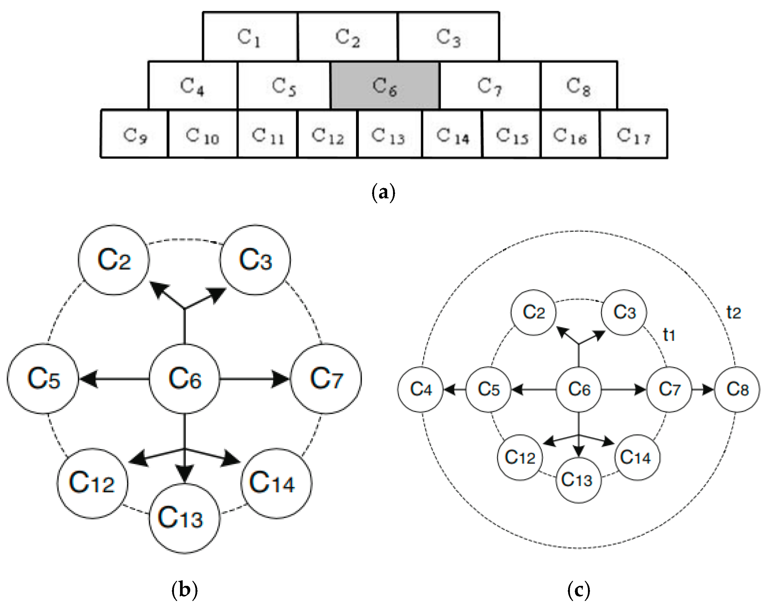
In order to better understand these concepts, a simple example illustrated by the authors of the method is shown. Consider the C
6 component as a target component of
Figure 3a (for simplicity, it is considered a two-dimensional case, but similar reasoning can be done even in the three-dimensional case) [
11].
In this case, the C
6 component has four possible ways in which it can be removed: Up, down, right or left. The first disassembly wave at the instant t
1 hits the components C
2 and C
3 at the top, C
7 at the right, C
14, C
13, and C
12 at the bottom, and C
5 at the left. C
6 can be considered 1-dependent with respect to C
5 or C
7, whereas it is considered d-dependent with respect to the other components. To remove the C
5 and C
7 components, it is necessary to also remove C
4 and C
8 (components that are involved by a second disassembly wave at the instant t
2) (
Figure 3b,c).
Thus, four possible disassembly sequences are obtained:
S1 = C2, C3
S2 = C8, C7
S3 = C12, C13, C14
S4 = C4, C5
2.1.3. 2nd Method: “Partial-Parallel Disassembly Sequence Planning for Complex Products”
This method, presented by Fei Tao, Luning Bi, Ying Zuo and A.Y.C. Nee, allows the planning of partial and/or parallel disassembly sequences using a DPM (disassembly precedence matrix), i.e., a matrix of disassembly precedences designed to improve the efficiency of the sequence with which the various parts are removed. This method considers a nondestructive disassembly of components and fasteners [
12].
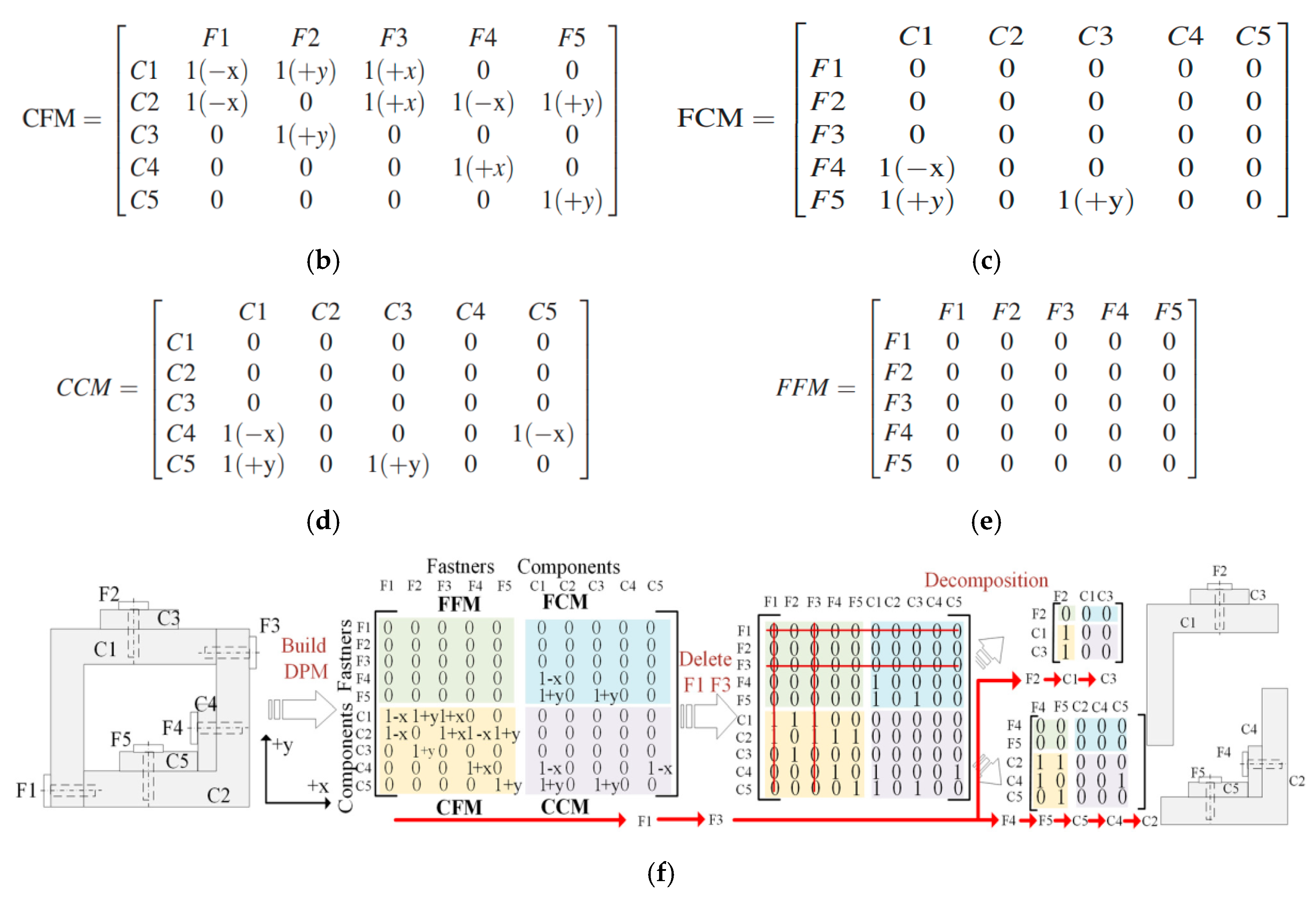
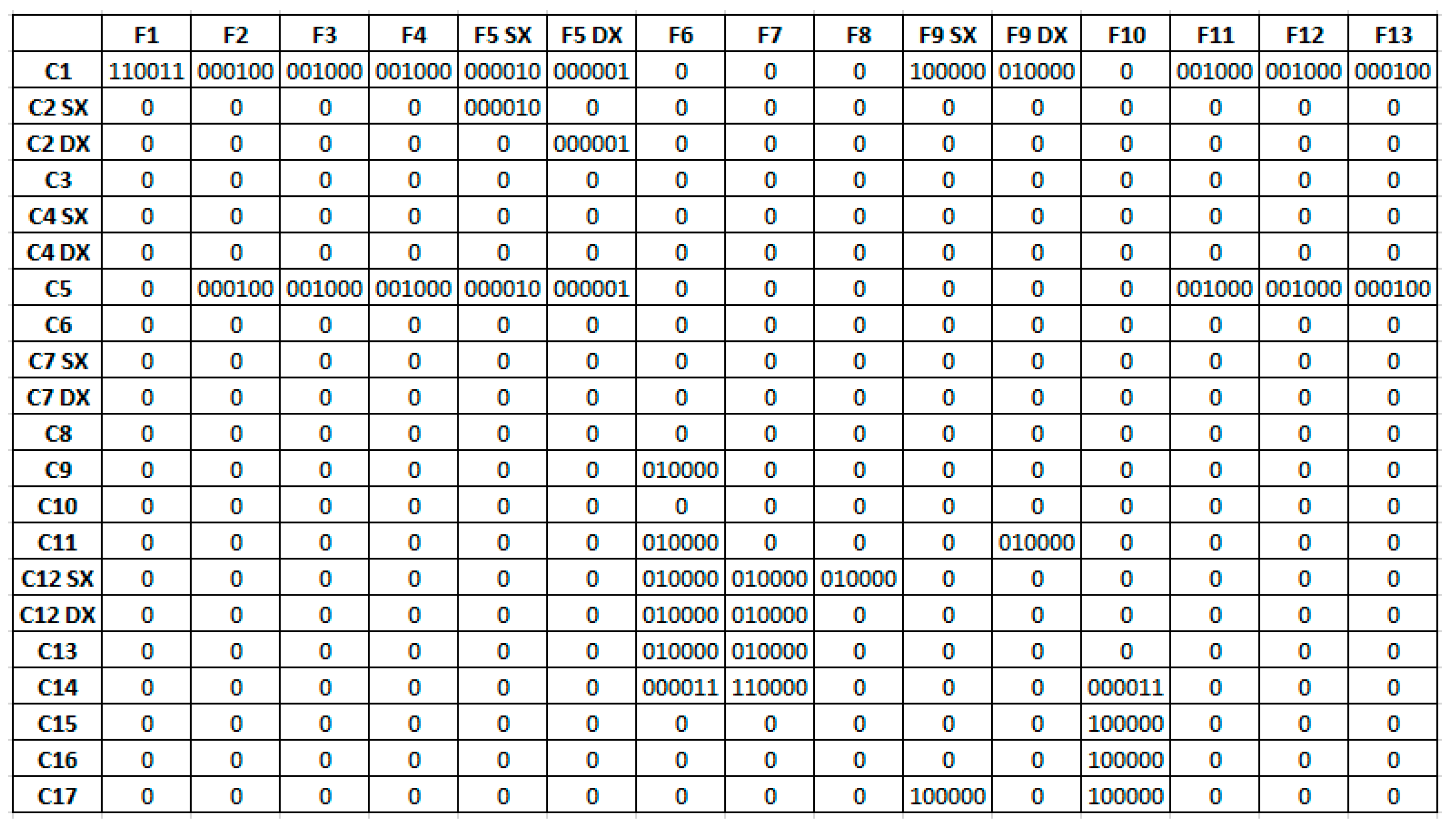
The DPM is made up of four submatrices: The CFM, the FCM, the CCM, and the FFM. The first thing to do, therefore, is the drafting of these submatrices.
In the CFM (components fasteners matrix), the vector of the j-th row represents the limitations due to the presence of the fasteners that the component j has along the directions in which it can be removed (if we are in a two-dimensional space, the possible directions are −x, + x, −y, and + y, while in a three-dimensional space, we also have −z and + z). If a fastener prevents the movement along the removal direction of the j component, 1 will be inserted in the corresponding cell, otherwise 0. Therefore, if 1 is present in a certain cell, it means that the component is blocked by the fastener, whereas if 0 is present, the component is not blocked by the fastener along the direction in which it is removed.
In the FCM (fasteners components matrix), the vector of the i-th row represents the limitations to which fastener i is subjected due to the presence of one or more components along the possible directions of removal of the fastener. If 1 is present in a cell, the fastener is blocked by the component, whereas if 0 is present instead, the fastener is not blocked by the component along the direction in which it is removed.
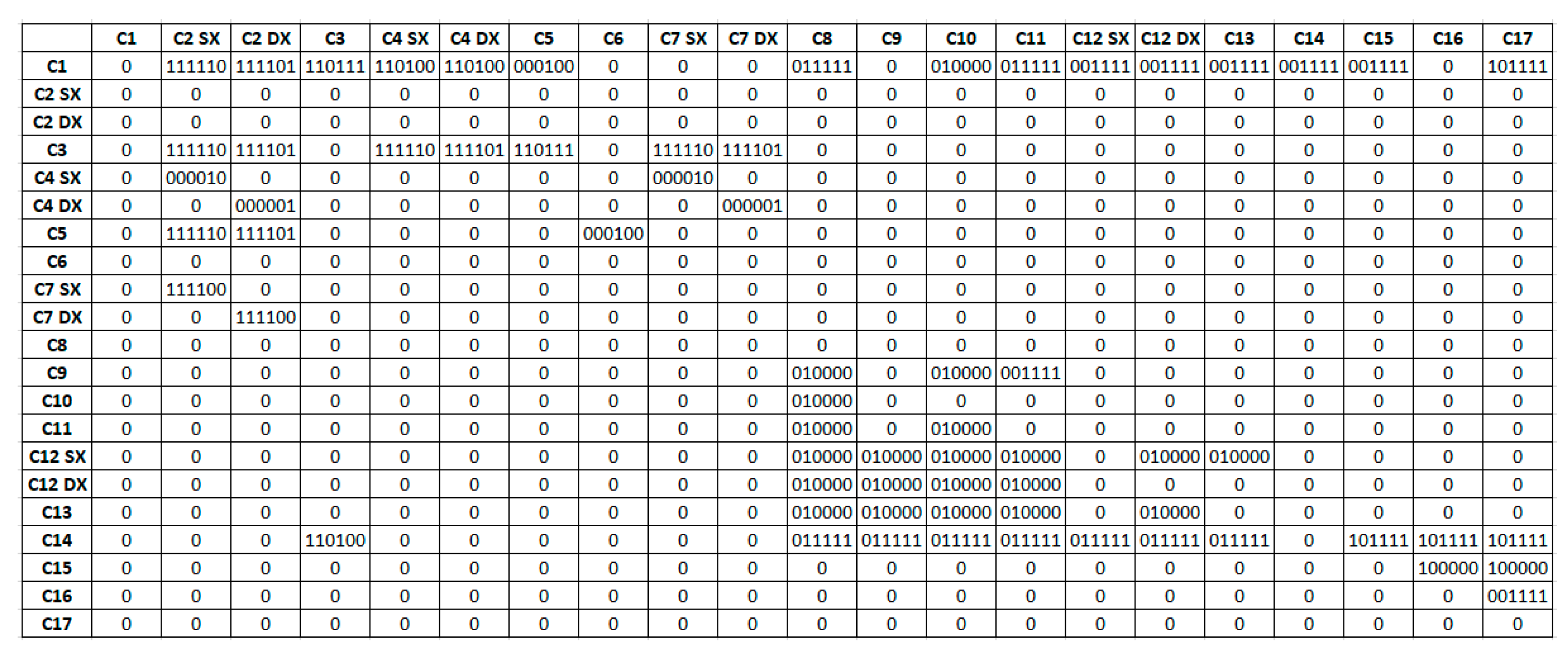
In the CCM (components components matrix), the vector of the j-th row represents the limitations to which the component j is subjected due to the presence of other components along the possible directions of removal of the component j. Thus, if there is 1 in a cell, the j component is blocked by another component, whereas if 0 is present instead, the j component is not blocked by another component along the direction in which it is removed.
The FFM (fasteners fasteners matrix) represents the precedence of disassembling between two fasteners: If 1 is present in a cell, movement of fastener i is prevented by another fastener, while if there is 0, the fastener i is not blocked by another fastener along the direction in which it is removed.
Unlike static DPM that does not change during the disassembly process, the DPM proposed by the authors is dynamic. In fact, it is modified every time a component or fastener is removed. When an element is removed, the corresponding row and the corresponding column are deleted, thus passing from a matrix that contains (m × n) elements to one that contains ((m − 1) × (n − 1)), indicating with m the number of rows and with n the number of columns. Furthermore, in disassembling any modules, considered as subassemblies, the DPM is divided into two or more sub-DPMs, each representing a new branch for disassembling. This dynamic system helps to reduce the size of the DPM and reduces the difficulty in finding feasible solutions.
To know when to remove a fastener or a component, two simple rules are used.
Rule 1 (disassembly of a fastener): The i-th fastener (indicated with Fi) can be removed when FCM (i,:) = 0 and FFM (i,:) = 0, where FCM (i,:) = 0 means that there are no components that block Fi along the disassembly direction, whereas when FFM (i,:) = 0, there are no other fasteners that have priority over Fi.
Rule 2 (disassembling a component): The j-th component (indicated with Cj) can be removed when CFM (j,:) = 0 and CCM (j,:) = 0, where CFM (j,:) = 0 means that all fasteners used to fix Cj have already been removed, whereas when CCM (j,:) = 0, there are no more components blocking Cj along the disassembling direction.
To these two rules we can add a third rule in the case where we have to disassemble a module, where by module we mean a set of components and/or fasteners connected to each other. If the product is separated into modules during the disassembly process, it is then possible to disassemble the modules in parallel, thus reducing the overall execution time.
Rule 3 (disassembly of a module): In a module, the previous relationships between the parties become internal limitations. If there are no other 1 in the corresponding DPM lines except for internal limitations, the module can be removed and disassembled into the individual parts.
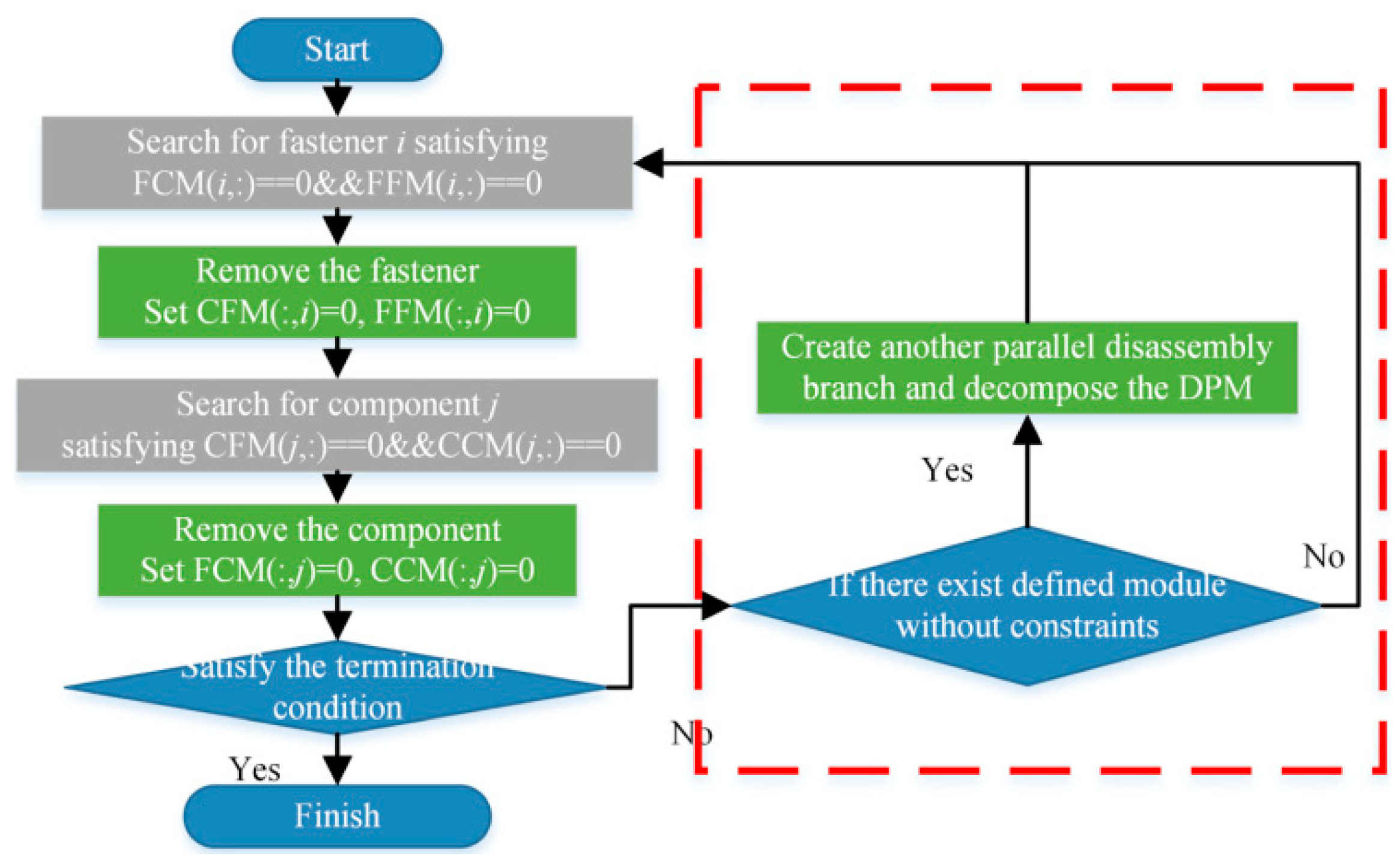
To generate a partial/parallel disassembly sequence, you need to follow five steps.
Step 1: Randomly generate a disassembly sequence of the fasteners. The random generation system ensures that all possible solutions/combinations are found.
Step 2: Disassemble the fasteners one at a time in the sequence order generated in Step 1. If the current fastener meets Rule 1, remove the fastener and go to Step 3, otherwise go to the next fastener.
Step 3: Remove all components that meet Rule 2.
Step 4: If the disassembly comes to an end (the achievement of the target component in the case of a partial disassembly), the final sequence is obtained. If not, go to Step 5.
Step 5: Check if there are any modules that satisfy Rule 3. If they exist, disassemble them in parallel, otherwise return to Step 2.
The main advantage of this method is to offer the possibility of obtaining different disassembly sequences which, if properly implemented, can offer an optimal solution with respect to a specific objective function. In fact, once a disassembly sequence is obtained starting from a certain order with which to try to remove the components, just modify this order to obtain a final sequence that is probably different from the previous one. If we go to iterate all possible initial combinations (i.e., all the different ways in which to try to remove the fasteners), we will get all the possible disassembling sequences for a given product (obviously according to the rules above) (
Figure 4).
On the other hand, however, obtaining these results in the case of a complex product is long and demanding, which is why it would be necessary to use a computer that is able to perform the operations automatically.
To better understand the concepts introduced above, an example illustrated by the authors of the method is presented. For simplicity, a two-dimensional case is taken into consideration, but similar reasoning can also be made in the three-dimensional case. Starting from the product illustrated in
Figure 5a, the matrices CFM, FCM, CCM, and FFM are made.
In CFM, for example, it can be seen that C1 is blocked by F1 in the −x direction, while in FCM, it is noted that F5 is blocked by C1 in the +y direction. Moreover, in the CCM, we can see that C3 is in the direction of removal +y of C5, while from the CCM, we deduce that there are no constraints between the fasteners because there are only 0.
At this point, the DPM can be created by “joining” the four matrices previously obtained. It is therefore decided to try to remove the fasteners in the following order: F1, F3, F2, F4, and F5.
The first fastener to be removed is just F1 because it satisfies Rule 1: This involves deleting from the row and the column of F1. Since it is not possible to disassemble any of the components, F3 is removed, eliminating the respective row and column. At this point, there is the possibility of separating the product into two modules: (F2, C1, C3) and (F4, F5, C2, C4, C5). These modules will be disassembled separately. If, however, as an initial sequence with which to try to remove the fasteners, we decided to use F1, F2, F3, F4, F5, it would not have been possible to divide the product into modules, and we would have obtained a different final sequence.
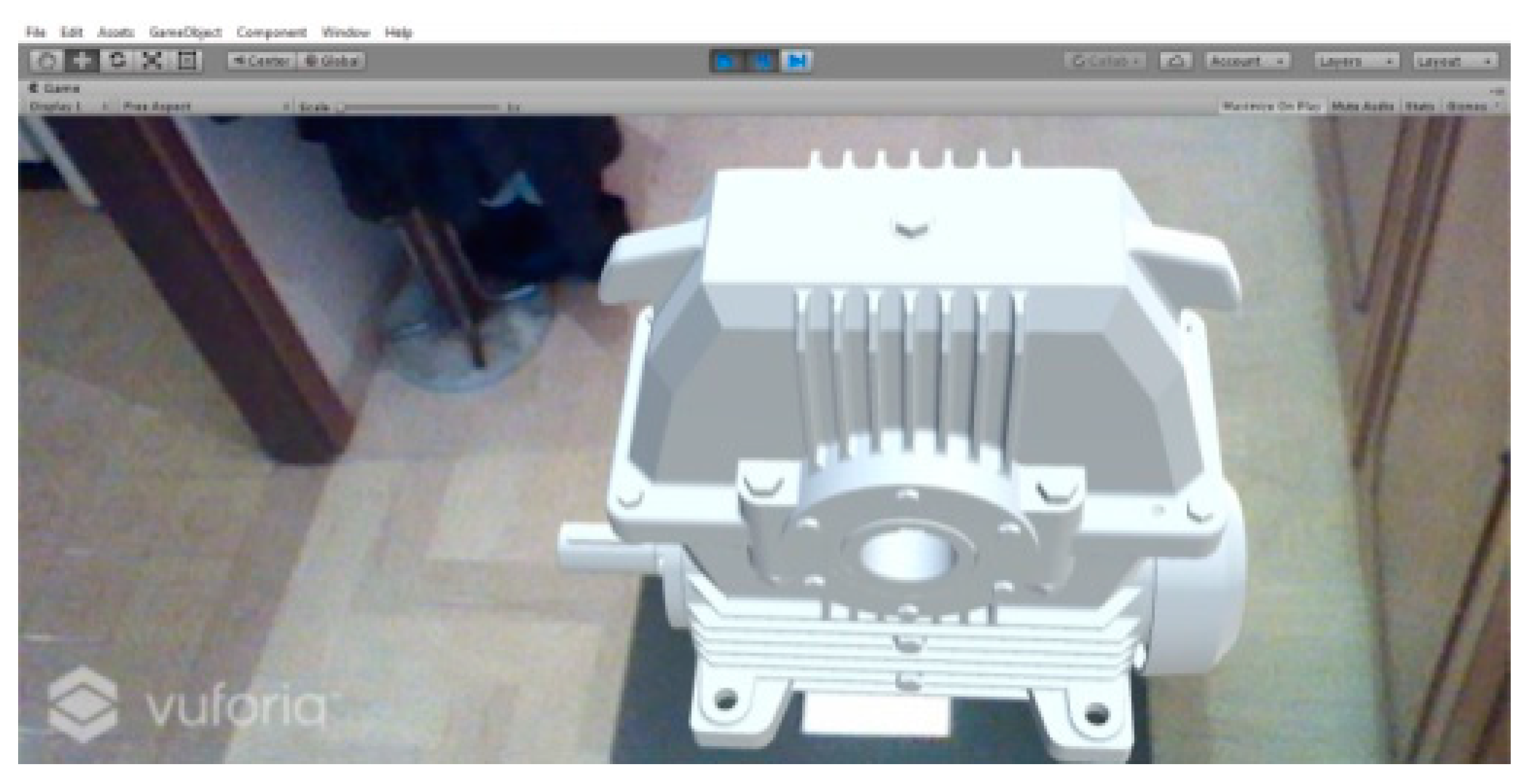
2.1.4. Application of Design for Disassembly to the Case Study of a Speed Gearbox
A case study is now illustrated in order to better understand and apply all the concepts presented up to now. To this goal, we decided to represent a speed gearbox through a 3D modeling program, thus orienting ourselves towards the metalworking sector. Then we applied the above methods to the gearbox mentioned, obtaining two different disassembly sequences. To these two sequences, we added a third one that we invented after choosing some logical criteria with which to obtain it. To better understand the advantages that design for disassembly offers, we finally made a comparison between the three sequences, evaluating them first according to the temporal criterion and, subsequently, by performing an economic analysis [
13].
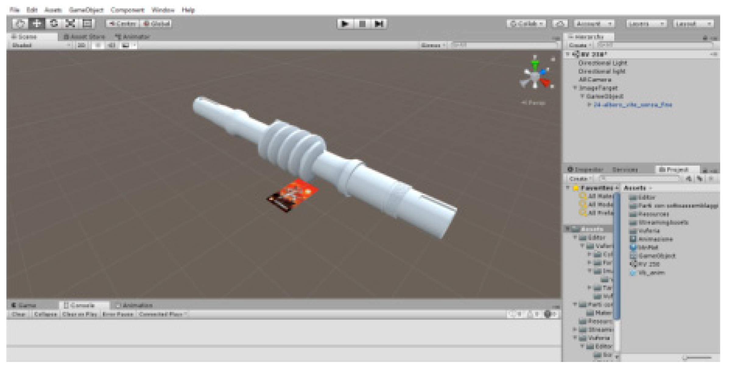
2.1.5. 3D CAD Modeling
For the 3D representation of the gearbox, it was decided to use a 3D CAD Modeler, i.e., Solidworks (version 2016), which is a CAD software (computer aided design) developed by Dassault Systèmes, used to draw and for three-dimensional design parametrics. We selected Solidworks because it is a program created specifically for mechanical engineering, and its use is quite intuitive. Moreover, it is possible to find various sources of information on the Internet (for example, forums and video tutorials) that allow easily acquiring greater knowledge about the software.
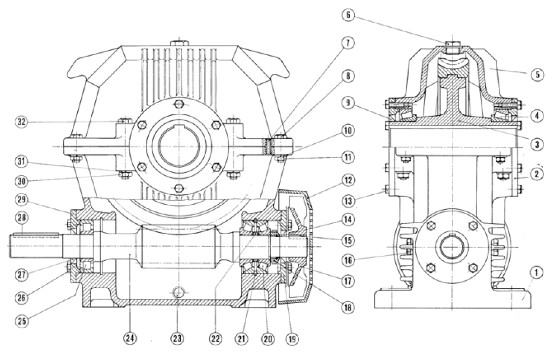
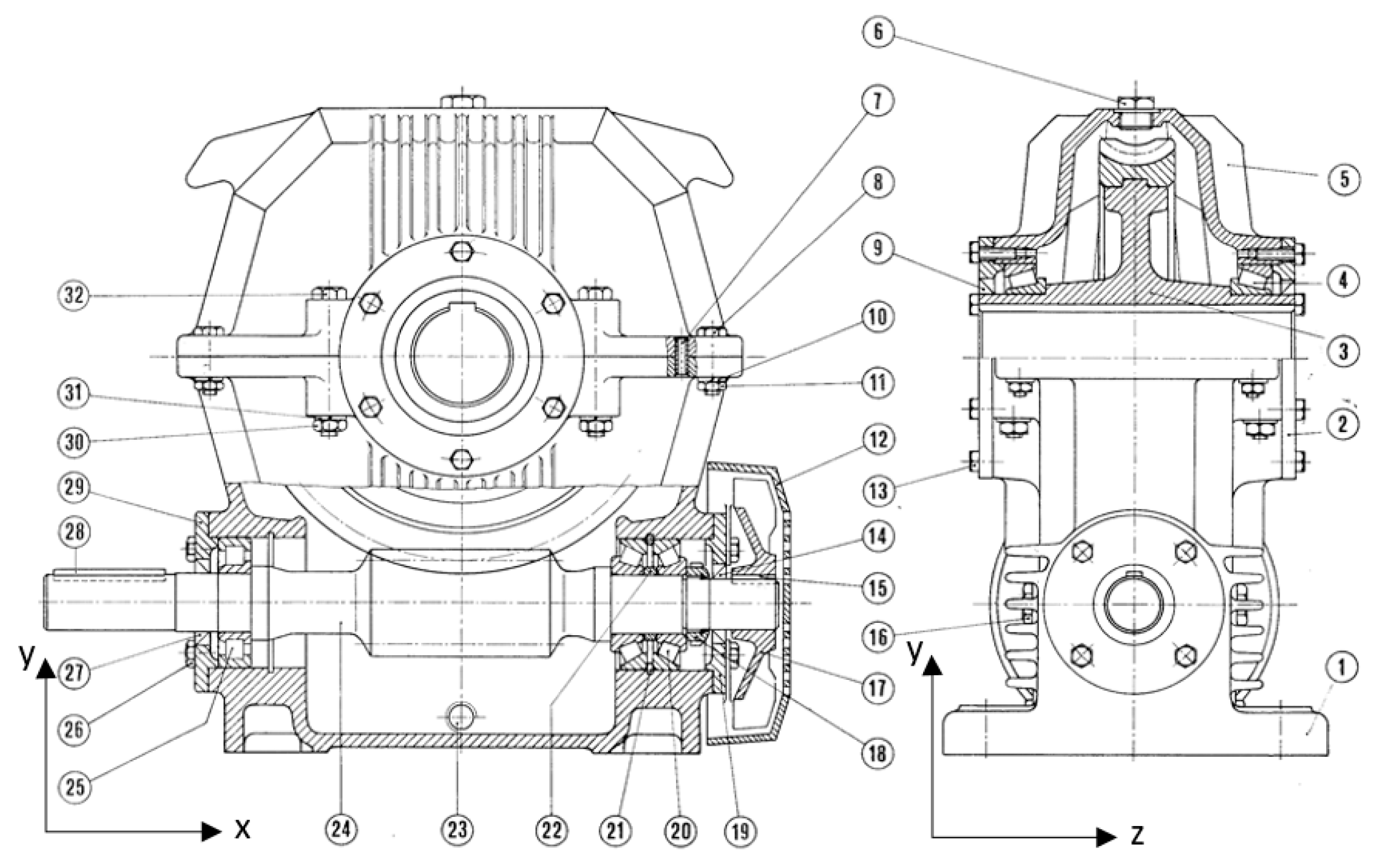
The gearbox represented is the RV 250 screw gearbox of the Rossi Motoriduttori Soc. of Modena (
Figure 6). Starting from the assembly (represented in 2D), we obtained the bill of materials (BOM), and then we made every single component in 3D, finally obtaining the gearbox in question by assembling the various components and inserting the properties and the relative constraints between them.
About the bearings, in the bill of materials, we have written in brackets the name of the models produced by SKF (a leader company in bearings production): Subsequently, we downloaded the relative models from the company’s website and used them for study’s purposes (
Table 1).
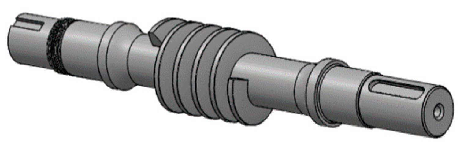
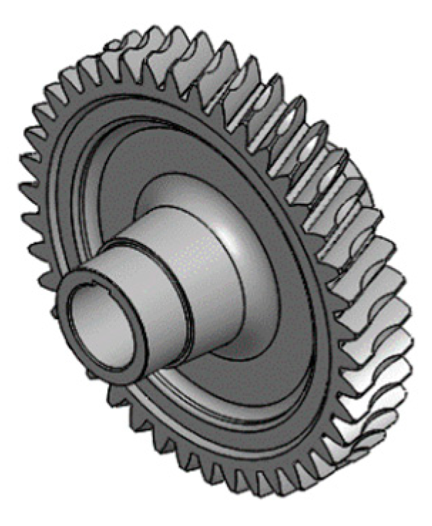
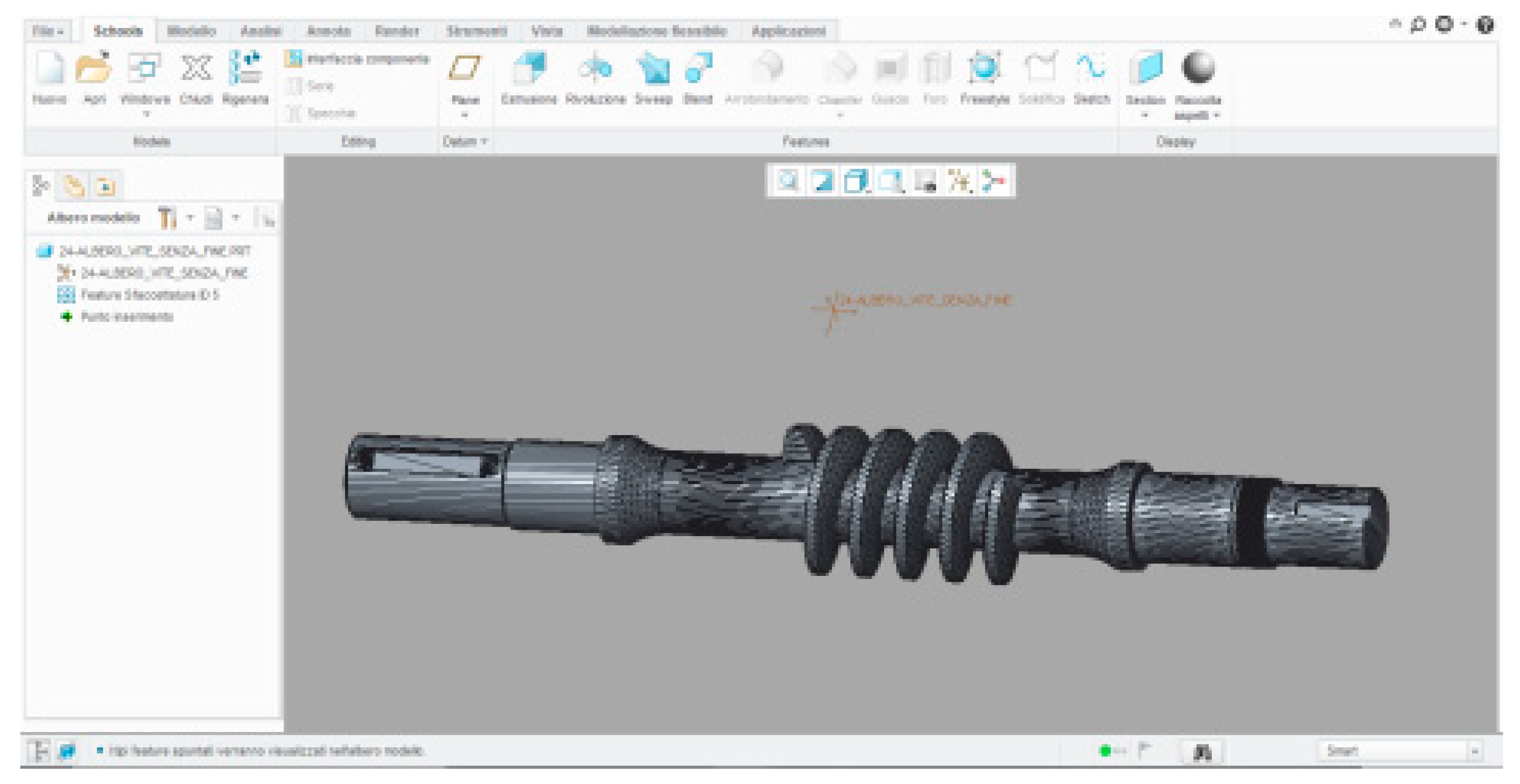
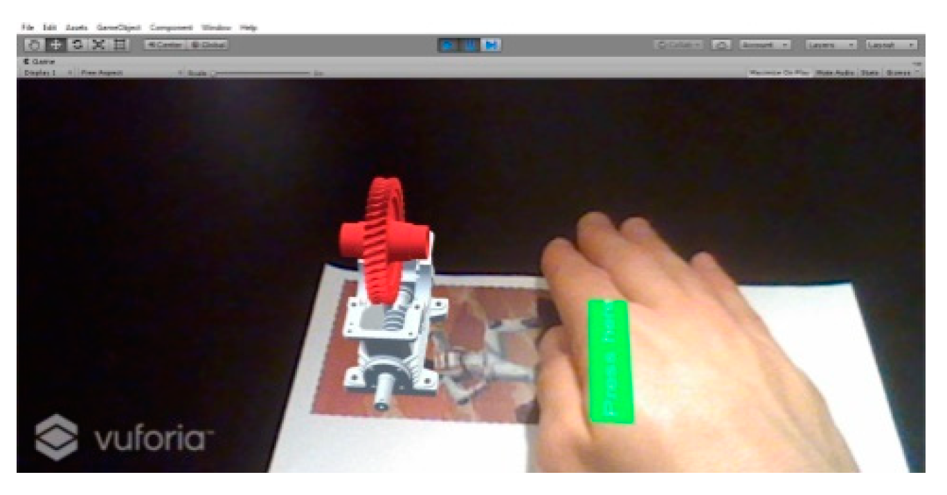
It is important to pay attention to the transmission shaft with endless gear and to the helical toothed wheel, as they are the two most important components because they are responsible for the motion. The screw gearboxes, in fact, are able to connect shafts with skewed axes (i.e., not belonging to the same plane and, therefore, not parallel to each other): Generally, the toothed wheel is the conducted element and engages on an endless screw, which acts as a driving force.
In order to realize the profile of the endless screw, the “extrusion with sweep” function was used, supplying the profile of an involute tooth as a profile and a helix path, while to make the teeth of the toothed wheel, the “cut with sweep” function was adopted, using as the profile that of an evolving tooth and as the path a segment of the required length and inclination (
Figure 7 and
Figure 8).
The constructive data of the screw and the wheel are shown below (
Table 2), as well as a representation of their assembly.
Using the data provided, we obtained other useful information to represent the components:
| Addendum | ha = mn |
| Dedendum | hf = 1,25 mn |
| Tooth height | h = ha + hf |
| Diameter of the foot | df = dm − 2 hf |
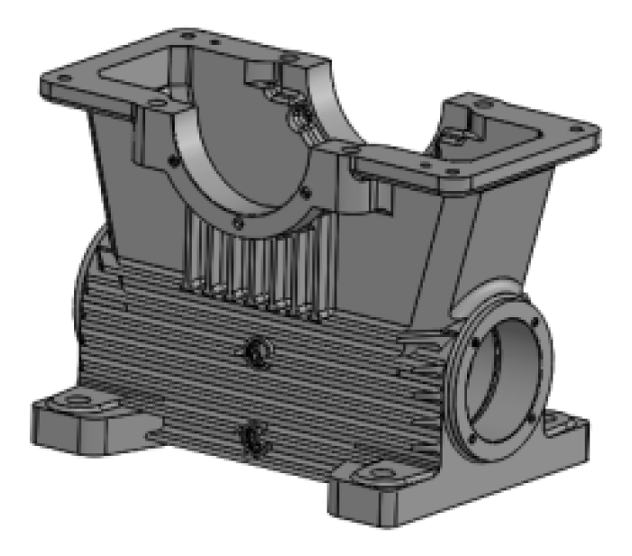
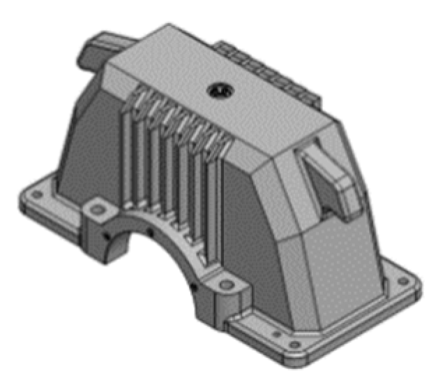
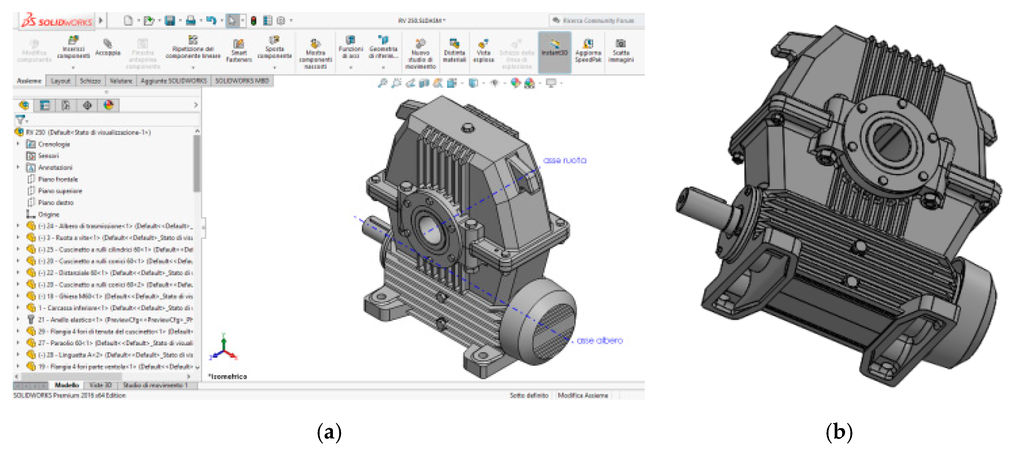
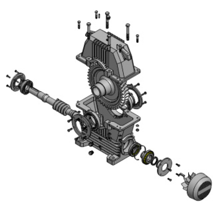
In the following figures (
Figure 9 and
Figure 10), some images of details of the assembly (in
Figure 11a, it is also possible to notice the software interface) and of the exploded view (
Figure 12) are shown instead.
2.1.6. Application of the First Method
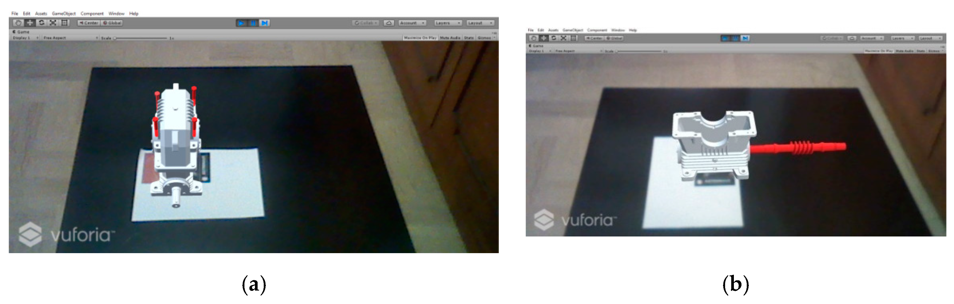
In this paragraph, the first method presented about the design for disassembly is applied to the case study. We wanted to perform a disassembly that allowed us to remove the drive shaft with an endless screw, which was considered our target component. The choice of the screw as a target component is reasonable because it is one of the components most subjected to stress and wear. For this reason, it is more likely that it will fail or in any case be replaced to perform preventive maintenance. In order to remove the shaft, the lower casing was not taken into consideration as it provides the support base to our gearbox, and the screw is contained inside.
Let us consider, as a first step, the oil drain at the lowest level, thus allowing us to disassemble safely. Then, remove the lower drain plugs, one on the left and one on the right. It is not necessary to remove the two upper drain plugs, which is why they were not considered and were not separated from the lower casing.
From
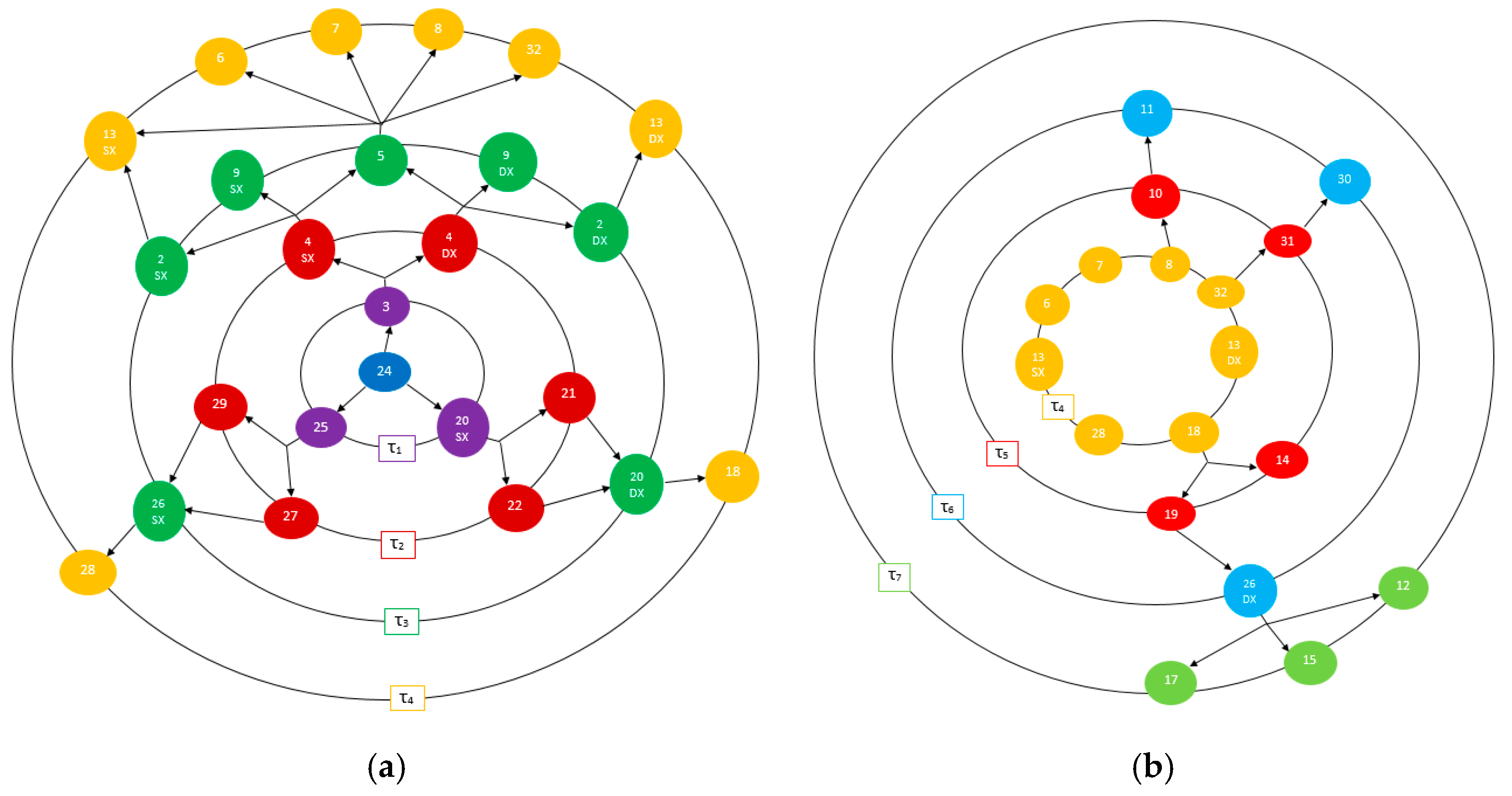
Figure 13a,b, it is possible to observe the expansion of the disassembly wave in the various instants τ.
The disassembling sequence obtained is as follows: 16 SX INF, 16 DX INF, 12, 17, 15, 26 DX, 11, 30, 31, 10, 19, 14, 18, 28, 8, 32, 6, 7, 13 SX, 13 DX, 2 DX, 2 SX, 9 SX, 9 DX, 5, 20 DX, 26 SX, 29, 27, 4 SX, 4 DX, 22, 21, 3, 20 SX, 25, 24.
In the disassembly sequence, the numbers are representative of the components and fasteners according to the numbering shown in the bill of materials (
Table 1). Moreover, for the sake of simplicity of reading, it was implied that when an element which is present several times is removed in the gearbox, in reality, that element is removed as many times as those it is present: For example, when an M20 nut (number 30) is unscrewed, in reality, we proceeded by unscrewing all four M20 nuts present. Finally, for those components or fasteners indicated together with the wording DX (right) or SX (left), the reference is given with respect to the overall starting drawing (
Figure 6).
Observing the result obtained, it can be noticed how this method leads to a complete disassembly of the gearbox.
2.1.7. Application of the Second Method
To apply the second method of design for disassembly to the case study, we started with the construction of the four submatrices, as well as the DPM. The general considerations made for the first method (target component, removal of the lower caps, numbers indicating the elements, etc.) also apply to this second method. First of all, however, a subdivision between components and fasteners is necessary, and the direction of removal of each element must be identified. In
Table 3, it is possible to observe how the components and fasteners have been grouped and renamed, in addition to the relative removal verses.
The removal directions are indicated numerically, represented with 1 if it is possible to remove an element along that determined direction, or with 0 if it is not possible. The order in which the directions are shown is as follows: −x, + x, −y, + y, −z, + z. If, for example, we want to represent the possibility of removing a component along the +x direction, we would write 010000 (
Table 4).
It was decided to orient the axes in the way shown in
Figure 14.
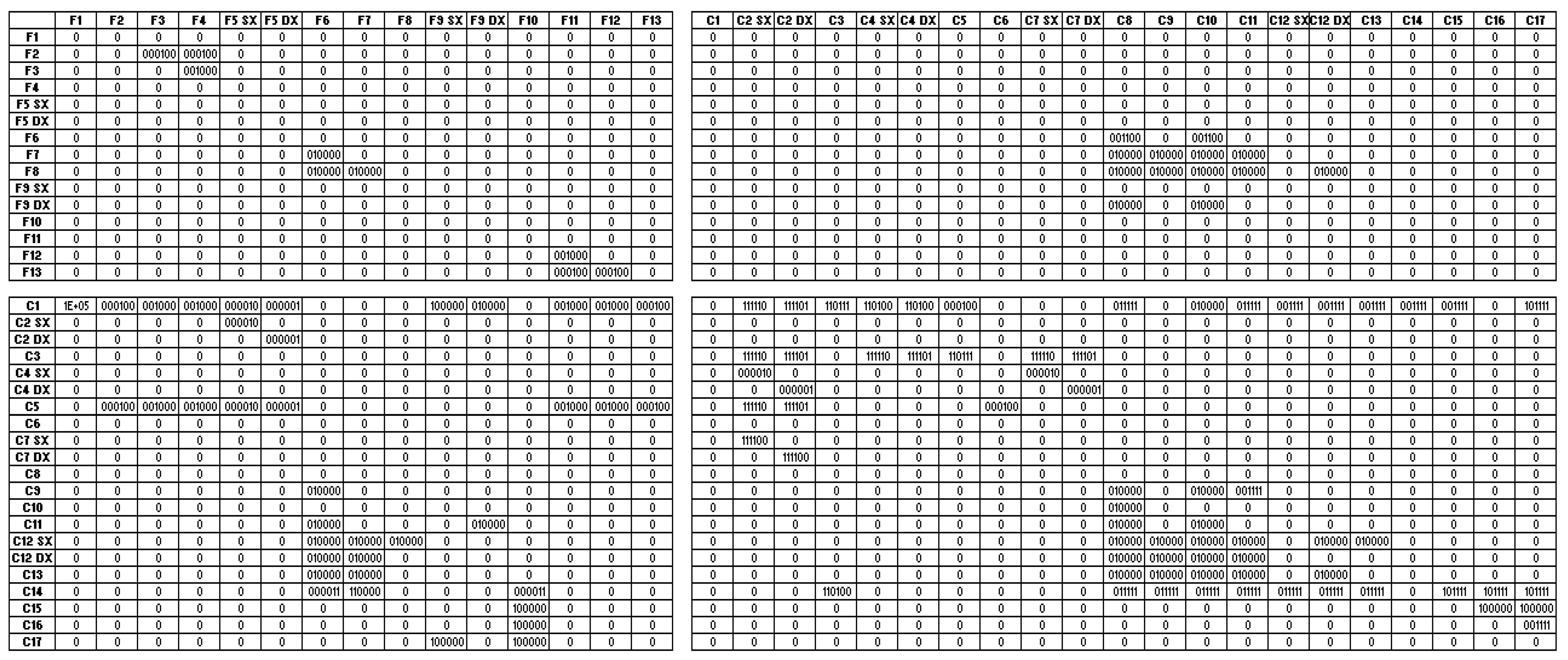
From the four submatrices, we can get the DPM (
Figure 19). A random sequence is chosen to try to disassemble the fasteners. In our case, this sequence is:
F1, F2, F3, F4, F5 SX, F5 DX, F6, F7, F8, F9 SX, F9 DX, F10, F11, F12, F13 (i.e., we try to remove the fasteners in the order in which they are presented in
Table 3b). Following this order, we note that F1 is the first DPM fastener with only 0 along the line, which is why it can be removed, together with the corresponding row and column. Subsequently, it is checked whether there is the possibility to remove one or more components (in this case C6) and then proceed following the rules of the algorithm previously illustrated. Towards the end of the procedure, it is interesting to note how the algorithm leads to the creation of two modules: M1 = (C1, C14) and M2 = (C3, C5).
Although the method provides for the parallel disassembly of M1 and M2, in our case, it is not necessary to disassemble M2, since the target component C14 belongs to M1. Furthermore, disassembling M2 in parallel would require the presence of a second operator, with a consequent increase in costs for carrying out an operation that is not necessary for our purpose.
The disassembling sequence obtained is the following (nomenclature with differentiation between components and fasteners):
16 SX INF, 16 DX INF, F1, C6, C8, C10, F4, F3, F2, F5 SX, C2 SX, C7 SX, C4 SX, F5 DX, C2 DX, C7 DX, C4 DX, F6, F9 SX, F9 DX, C11, C9, F7, C12 DX, C13, F8, C12 SX, F10, C17, C16, C15, F11, F12, F13, M2, C14.
Then, we obtain the equivalent sequence (nomenclature with numbering of the bill of materials): 16 SX INF, 16 DX INF, 7, 6, 12, 17, 11, 10, 8, 13 SX, 2 SX, 9 SX, 4 SX, 13 DX, 2 DX, 9 DX, 4 DX, 15, 26 SX, 26 DX, 19, 14, 18, 20 DX, 22, 21, 20 SX, 28, 29, 27, 25, 30, 31, 32, M2, 24.
Observing the sequence obtained in this case, differently from the result obtained with the first method, we note that we did not carry out a complete disassembly of the reduction unit thanks to the generation of the M2 module which was removed without being further decomposed.
2.1.8. Sequence Created by the Authors
The sequence hypothesized by the authors was realized on the knowledge of the gearbox that was acquired during the three-dimensional modeling phase. Authors relied mainly on intuition and common sense in addition to experience. The general considerations made for the other two methods also apply in this case.
First of all, authors proceeded to remove the two lower drain plugs to allow the oil to escape. Then, they removed all the connecting organs that hold the upper casing together with the lower one. They considered the formation of a subassembly S1 consisting of the filler cap and the upper body: S1 = (5, 6). The loading cap was removed with the upper casing as it was not necessary to remove it individually to reach our target component (the worm shaft) and no particular complications were involved in the operations to be performed. The subassembly was then removed. The goal was to remove the screw by pulling it out of the right side of the casing, without completely disassembling the lower part. Once the tab 28 had been removed, the various elements located on the right side of the lower casing were removed, until we had reached our objective.
The sequence of disassembly obtained is as follows: 16 SX INF, 16 DX INF, 30, 31, 32, 11, 10, 8, 13 DX, 13 SX, 2 SX, 9 SX, 2 DX, 9 DX, 7, S1, 4 SX, 4 DX, 3, 28, 12, 17, 15, 26 DX, 19, 14, 18, 20 DX, 22, 21, 20 SX, 24.
During the disassembly, the authors tried to perform in succession the removal of components and/or fasteners that required the same work tool or that, depending on the case, were located on the same side of the gearbox, thus reducing the running time and fatigue to be done.
2.1.9. Calculation of Disassembly Times and Comparison of the Results Obtained
Now we want to evaluate the three disassembly sequences using the temporal criterion. Through the help of some tables, the time needed to complete the individual operations was estimated and the sequence that requires the least time to disassemble was sought.
For the estimate of the disassembly times, the authors referred to two essays: The first is “Disassembly Analysis through Time Estimation and Other Metrics” by Ehud Kroll and Brad S. Carver, while the second is “Evaluation of Disassemblability to Enable Design for Disassembly in Mass Production” by Anoop Desai and Anil Mital. The method adopted consists of an indirect estimate of the times. The focus is in fact placed on some parameters such as the structural aspect of the parts (e.g., symmetry, size, weight, center of gravity), the organizational aspect of the parts (e.g., product structure, standardization, variability), the pre-process (e.g., work space, information on disassembly, degree of automation) and the in-process (e.g., direction of disassembly, hand mechanisms, interference).
After defining some influencing factors of disassembly, a quantitative assessment was provided by assigning scores in TMU (time measurement unit). For this phase, the tables in Anoop Desai and Anil Mital’s essay [
9] were taken as a reference.
First of all, for each element, you define which task you want to perform (unscrew, push, open, etc.) and with which tool this operation is performed (by hand, with a screwdriver, with a key, etc.). The function that the various parts play after being disassembled is then defined: In fact, at the end of their life (EOL), they can be recycled (recycling), regenerated (remanufacturing) or reused (reuse). In cases where they are recycled, only the material of the components is still used to perform other functions, and therefore, it is necessary to bear costs related to disassembling, cleaning, and recycling. If the components are regenerated instead, they are disassembled from the product structure and are subject to a technological redesign that allows increasing or simplifying the performance: In this case, the costs to be incurred are those related to disassembly, cleaning, redesign, and working to revitalize them and to assemble them again. Finally, a component subject to reuse is disassembled from the product structure and is reused as is, without undergoing technological improvements or redesign: The costs to be incurred are those related to disassembly, cleaning, and assembly.
Once the function that elements acquire after the disassembly is indicated, proceed with the assignment of the scores in TMU referring to [
9]. It can be seen that in the paper, several factors that influence disassembly can be taken into consideration, such as: The disassembling force (the lower the amount of force, the lower the amount of effort to be made), the movement of the material (a smoother grip of the component implies less time taken), the use of tools (ideally, you would like to disassemble without the use of tools, but in practice we try to minimize the number of necessary tools), accessibility (easy access to components and fasteners is essential for fast and efficient disassembly), and positioning of the working tool (the lower the precision required from the instrument, the less time will be used).
Concerning the case study of the gearbox, the authors decided to allocate all components and fasteners to reuse, except for the transmission shaft with the worm screw, which was destined for recycling. To obtain the time estimate of the disassembly sequences, it was sufficient to multiply the value in TMU by 0.036 (1 TMU = 0.036 s). It can be seen how the sequence obtained with the first method corresponds to a value of 9415 TMU (corresponding to 338.94 s) and how this value is the highest among the three sequences made: In fact, the sequence obtained with the second method had a score of 9324 TMU, which corresponds to 335.66 s, while the sequence devised by the authors had a score of 8255 TMU, corresponding to 297.18 s. The sequence obtained with the first method is the longest since it has led to a complete disassembly of the gearbox, unlike the other two which, by contrast, are faster because we reduced the number of elements to be disassembled. Finally, we can observe how the components and the fasteners did not have the same effect on the duration of the disassembly: The bearings, for example, were among the longest components to be removed due to their position, the use of tools, the force to be exerted, and the precision with which it was needed to operate, unlike nuts, rosettes or screws, which were disassembled in a short time because they were easily accessible and removable by applying a limited force.
2.1.10. Economic Analysis
To better understand the real advantages that design for disassembly offers, an economic analysis was carried out going to quantify the savings that you can have between the sequences identified in the case study. First of all, the authors had to quantify the cost that a company must support for one of its employees and, to this end, they referred to the data reported by the Italian Ministry of Labor and Social Policies (
https://www.lavoro.gov.it/temi-e-priorita/rapporti-di-lavoro-e-relazioni-industriali/focus-on/Analisi-economiche-costo-lavoro/Pagine/Settore-metalmeccanico-industria.aspx): The data in question are updated to October 2017 and refer to the workers belonging to companies in the private engineering industry and the installation of plants. Taking as a reference the values relating to a worker hired at the 4th level indefinitely, we can obtain the following data:
Average annual cost = €34,347.52; average hourly cost = €21.47; theoretical annual hours = 40 h * 52.2 weeks = 2088; hours worked average per year = 1600.
Considering one of the disassembly sequences, knowing the duration, we were able to calculate the number of pieces processed in a year and, subsequently, we obtained the unit cost. To compare the three sequences, the authors took the least productive one (that is the one made with the first method) and calculated the annual cost. Finally, the authors calculated the cost related to the production of an equal quantity of products made with the other two sequences and compared it with the cost related to the less productive case, thus obtaining the savings that we were able to obtain.
It can be seen how a good design of the disassembling sequence allows having no indifferent advantages on the economic side (in our case, we can save over €4000/year), also considering the fact that the sequence conceived by the authors (the most advantageous) is not said to be the best ever: If we continued to search for other possible disassembling sequences, we would probably have reached a sequence that was even more advantageous than this (
Table 5).


