Abstract
This paper addresses the identification and correction of amplitude and offset errors in the sinusoidal outputs from incremental position encoders. Precise angular position measurement is of high importance in many position control applications. Manufacturing tolerances and noise from thermal and electromagnetic interference sources introduce systematic and random errors in the orthogonal sine cosine output line signals. Evaluation of these signals reproduces deviations in the measured angular position. This paper proposes two methods to identify and compensate for the influence of the systematic errors online without the necessity of a reference measurement during identification. The key component of the methods is a nonlinear estimator that exploits the orthogonality property of harmonic functions. The first method explains the basic idea with a scalar error model and operates continuously but exhibits an angular shift in direction of rotation during transients of the parameters, whereas the second method assumes an error model with error parameters as a function over one full revolution of the encoder. The latter updates the error function iteratively in subsequent revolutions.
1. Introduction
Incremental position encoders are widely used for precise angle and speed determination in all kinds of motion control applications, where precise positioning is indispensable. The incremental encoder can be connected to the servo controller by either binary or analog sine cosine quadrature signals. Several controllers provide additional digital communication protocols, such as the proprietary protocols ENDAT [1], HIPERFACE® [2], or the open protocol BiSS [3]. Often, both a digital and analog interface is offered on the same device. In this paper, the evaluation of analog quadrature signals is discussed. Here, we assume that the quadrature signals stem from an optical device, but the methods described can also be applied to the evaluation of other quadrature sine cosine signals from magnetic devices such as resolvers or magnetic incremental sensors. This includes resolvers, but excludes other absolute encoders. In a motion control application, the feedback signals for the speed and position control loop are derived by interpolation from the quadrature signals. The evaluation can be grouped into three main groups [4]: (1) parallel paths for digitally counting encoder cycles after routing sine and cosine over comparators and acquisition of a high resolution angle information from the arctangent of sine and cosine analog values after discretization via high speed analog-to-digital converters; (2) using a phase locked loop to track the angle of the sine and cosine signals and counting overflows of as encoder line cycle advances; (3) analog-to-digital conversion by very fast converters, direct calculation of arctangent by fast signal processing (DSP or FPGA with a sampling time in the range of a one microsecond) and again counting overflows of as encoder line cycle advances. The second method is often, especially in conjunction with resolvers, implemented in analog-digital mixed signal processing and directly gives an analog speed signal. The first and third method usually apply time discrete digital differentiation to obtain the speed signal. Both methods rely on the correct sine and cosine curve shape of the quadrature signals. An optical incremental encoder has many entry points, where disturbances can be added to the signal output. Each channel employs at least two photo diodes to detect the positive and negative half wave of the sine. Mismatches of the diodes as well as incorrect calibration of the analog preamplifiers result in amplitude and offset errors. The optical scanner system is a very delicate mechanical construction. Imperfections in the optical design of the scanner unit and tolerances in the distance between grated disk and scanner unit or relative orientation errors also lead to offsets and amplitude errors, but can introduce harmonics in the sinusoidal curve shape and phase differences as well. The manufacturing tolerances of the grated disk influence the same error parameters. If the grating pattern on the disk is not centered with respect to its rotating point or mounting of the disk on the shaft is not perpendicular to the shaft, the design parameters of the optical system change with the mechanical revolution, and, subsequently, the same error pattern mainly results. Offset and amplitude errors generated by the lithographic production process for the disk can be global for the whole disk or also local, affecting only part of it. All errors mentioned so far are reproducible with the mechanical revolution and can be compensated, once the underlying parameters are identified and considered in the evaluation of the quadrature encoder output signals. Other influences, dependent on electromagnetic interference, electronic noise, mechanical strain or temperature can not so easily be compensated, unless the influence can be modeled and its cause detected.
Any deviation of the sensor output signals from the sine-respective cosine form distorts the angle measurement [5] and leads to position errors in the motion control, or increases, for example, an acoustic noise, because the speed controller tries to counteract this disturbance. The non ideal shape of the encoder output signals has to be considered in the angle evaluation electronics. An error model is set up to define the parameter structure of the error shape, and its parameters have to be identified for the individual measurement device. There are three groups of methods to identify the parameters of error models: In a first group a reference measurement encoder is used to obtain independent position information. Then, the deviations are recorded and processed to calibrate the error model. The second group relies on a constant speed test, where the device which is to be characterized runs at constant speed, i.e., with a high inertia on its shaft. Speed deviations are recorded and used to calibrate the error model. These first two groups are considered as offline methods because special measurement conditions apply for the identification process. A third group of online methods is independent of a separate adaption test under controlled conditions and are able to run under normal operating conditions online. Once the error parameters are known, a compensation can be applied by an inverted error model in the angle evaluation electronics.
Many approaches have been developed to cancel the adverse effects of the non-ideal line signals. Höschler presents in [6] an offline approach, which employs lookup tables. The true position is interpreted as a function of the uncorrected position that has to be recorded offline for every individual encoder using a precise reference encoder. Moreover long-term drifts and other effects could not be taken into account. Hwang [4] presents a method that uses the amplitude of the quadrature signals in the form of the square root from the sum of squared sine cosine signals, which is compared to its nominal value, and the difference is integrated by gated integrators, which are enabled in specific angular regions of the line cycle. The gating angular intervals are derived from the estimated angle. This method is from the online type. It compensates for the two offsets and the amplitude ratio between the line signals. Peterson [7] also uses the amplitude of the quadrature signals, but samples its value at angular points derived from the estimated angle. From these samples, the amplitude ratio and offset values for the two signals can be directly calculated and applied for the compensation. In [8], the erroneous line signals are corrected by using Radial Basis Functions in a two-stage neural network. Another approach based on oversampling was proposed by Kirchberger in [9]. His method filters the transformed line signals to perform the correction. Daaboul [10] describes an offline method based on a constant speed measurement with a two-stage compensation. In the first stage, the offset and amplitude values are identified and compensated. In a second stage, harmonics of the quadrature signals are identified but assumed to be identical in amplitude and phase for all cycles of the encoder. The compensation is performed also in two stages: after high speed analog-to-digital conversion, the further processing is carried out in an FPGA at a sampling rate of 10 MHz. In the first step, amplitude and offset of the two tracks are compensated with a table lookup over one full mechanical revolution. After atan2 calculation, an error lookup table, which spreads over only one line cycle, is used to compensate angle deviations caused by the harmonics of sine and cosine. In the paper [11], an approach based on the orthogonality of trigonometric functions is presented. It analyzes second harmonics on the squared magnitude of the line signals online and thereby derives the systematic error parameters for offsets, amplitudes and phase error. With the estimated errors, the line signals could be corrected. A second paper [12] proposes a structure of lookup tables, which are generated offline to interpolate the quadrature signals by calculating higher harmonics to form a quadrature system with a multiple number of cycles. The tables are generated in such a way that during the angle evaluation, offsets, a phase shift and amplitude errors are automatically compensated.
This paper defines an error model with just five parameters: DC-offset and total amplitude on tracks A and B of the encoder as well as phase shift deviation between tracks. We use a Harmonic Activated Neural Network (HANN) [13] to adapt the error parameter values online without a reference angular measurement. The general approach of the HANN is slightly modified and tailored to the application. The classical HANN relies on a reference measurement to obtain the ideal output signals, which it compares to the distorted signals from the encoder, whose parameters are to be identified. In this paper, we propose omitting the reference measurement and take the already precorrected estimate of the angle instead to calculate the ideal line signals in a kind of feedback loop or nonlinear observer. Throughout the paper, the nominal amplitude of the quadrature signals is assumed to be 1.
2. Systematic Errors on the Encoder Signals
An ideal encoder provides two line signals: line A follows a sine and line B a cosine with the same amplitude, which is supposed here to be 1. The position is calculated by counting the signal periods, which determines the coarse angle , and computing the atan2 function of the line signals within one cycle, which determines the fine angle ε. The coarse and the fine position, scaled by the number of lines N, added together yields the absolute position :
Due to manufacturing tolerances in the production of encoders, the line signals are erroneous, and this results in a faulty angle determination. In order to achieve a high quality angle acquisition, the parameters of an error model describing the systematic errors of the sinusoidal signals are estimated, and the inverse model is applied to compensate for the effect. The error model contains the parameters’ phase shift deviation between line signals and offset and total amplitude of both lines as written in (2) and (3). The offset errors are and , the erroneous total amplitude and , respectively, and the phase error , which describes the deviation from 90 degree phase-shift between both signals as described in [10]. The specified error parameters are assumed to be a function of the mechanical angle .
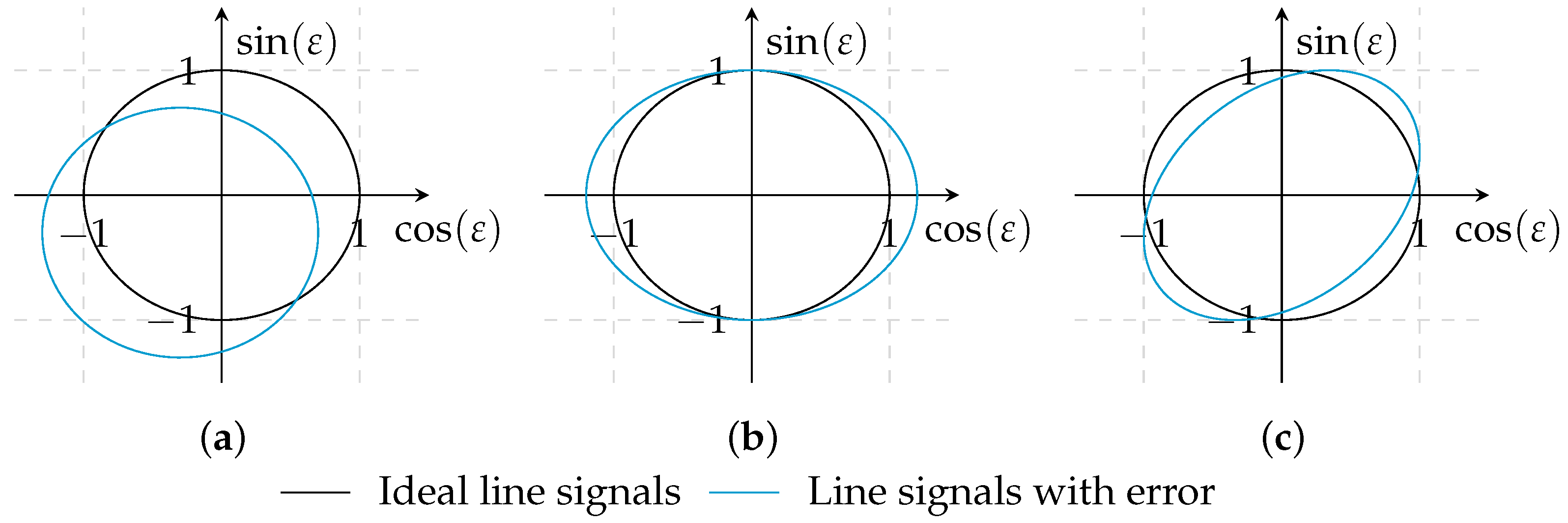
Figure 1 shows the impact of the different error types on the angle determination separately. The black line (  ) illustrates the ideal line signals without any errors, and it corresponds to a circle with radius 1 and a center in the origin. The resulting courses for individual error parameters are depicted in blue (
  ). Offset errors shift the origin as shown in Figure 1a. A deviation in amplitude deforms the circle into an ellipse parallel to one of the axes as shown in Figure 1b. The distortion in Figure 1c is caused by phase-shifted line signals.
) illustrates the ideal line signals without any errors, and it corresponds to a circle with radius 1 and a center in the origin. The resulting courses for individual error parameters are depicted in blue ( ). Offset errors shift the origin as shown in Figure 1a. A deviation in amplitude deforms the circle into an ellipse parallel to one of the axes as shown in Figure 1b. The distortion in Figure 1c is caused by phase-shifted line signals.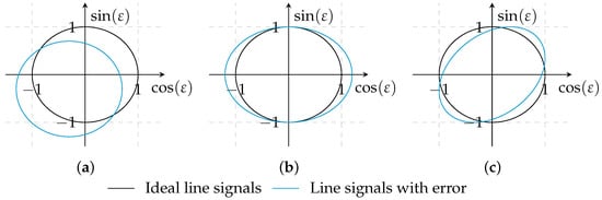
Figure 1.
Impact of (a) offset; (b) amplitude and (c) phase-shift errors on the angle determination.
3. The Harmonic Error Correction
The proposed method, known as Harmonic Error Correction (HEC), is able to estimate the parameters’ offset and total amplitude of the sinusoidal encoder signals, which affect the fine position of the encoder, as described in Section 2. Offset and amplitude are assumed to be constant over the whole mechanical revolution in the beginning. The phase shift deviation is neglected and set to zero further on in this paper. Therefore, the assumption (2) and (3) can be simplified to (4) and (5) and combined to (6). The offset and amplitude parameters can be concentrated to the vector (7):
3.1. Theoretical Structure
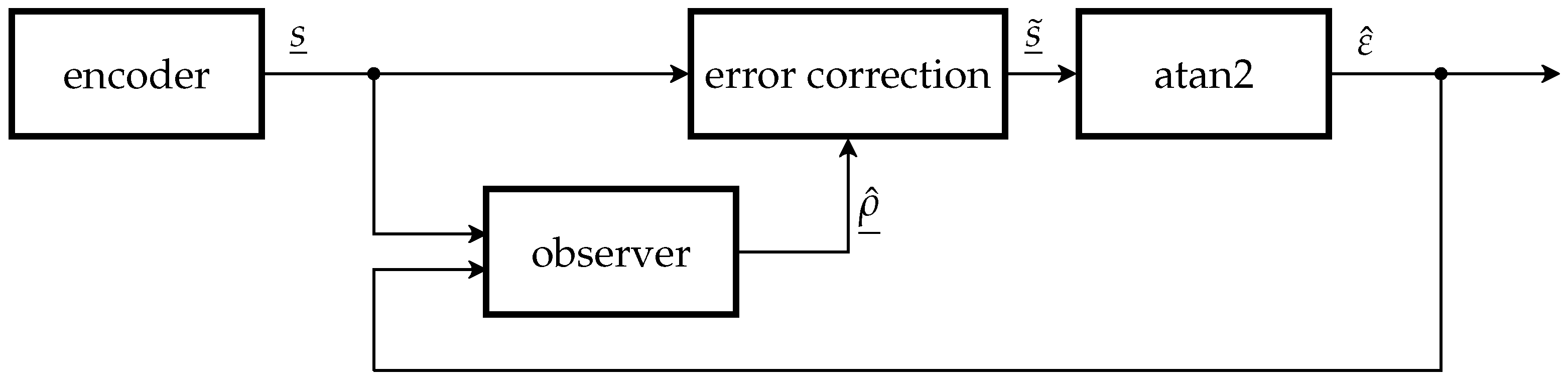
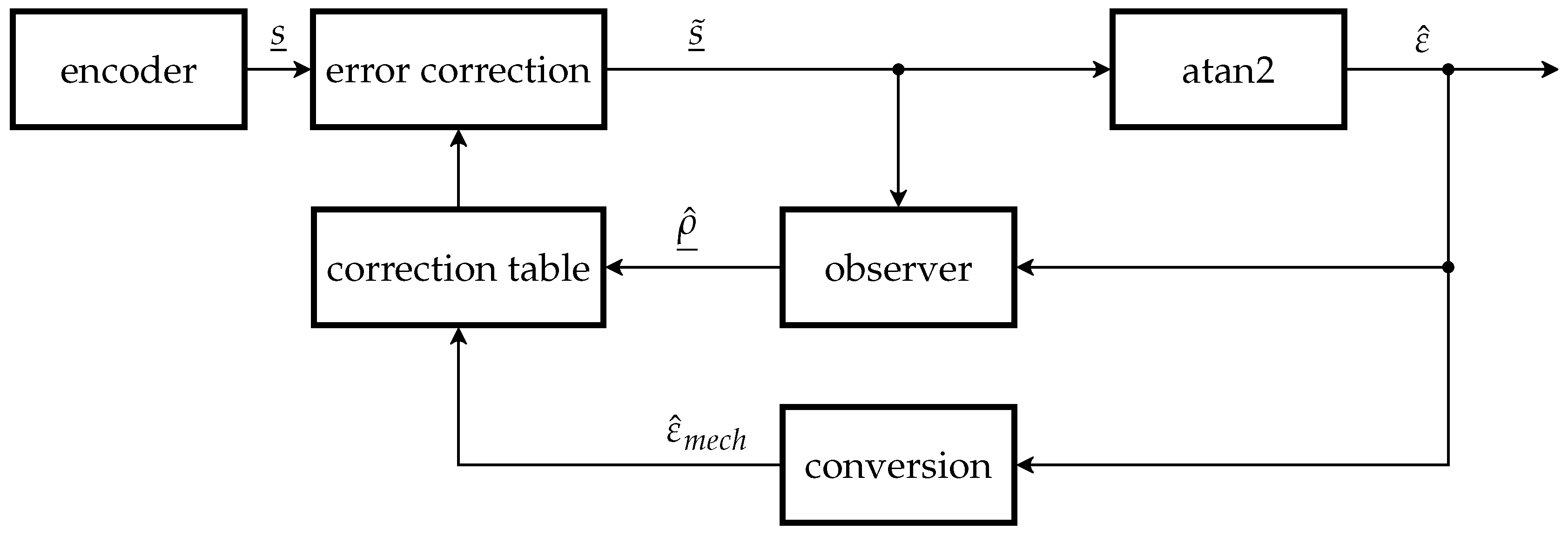
Figure 2 shows the scheme of the proposed error correction method. Throughout the paper, we use the variables without decoration (i.e., (6) and (7) ) for true values present in the encoder, variables with hat for quantities estimated by the observer (i.e., ) and variables with tilde (i.e., ) for measured signals corrected by an inverted error model with the estimated parameters. The nonlinear observer adapts the error parameters using the estimated angle and the line signals . The error correction block contains the inverted error model. The line signals are adjusted with the error parameters to obtain the corrected line signals . The atan2 function calculates the estimated angle from these corrected line signals.
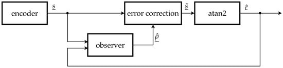
Figure 2.
Scheme of the proposed Harmonic Error Correction.
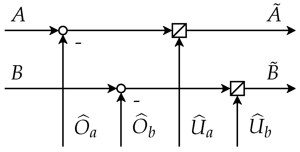
The error correction of the line signals is implemented by a subtraction and a division of the estimated error parameters , as pointed out by (8) and (9). The signal flow of the error correction is shown in Figure 3:
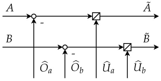
Figure 3.
Scheme of the error correction.
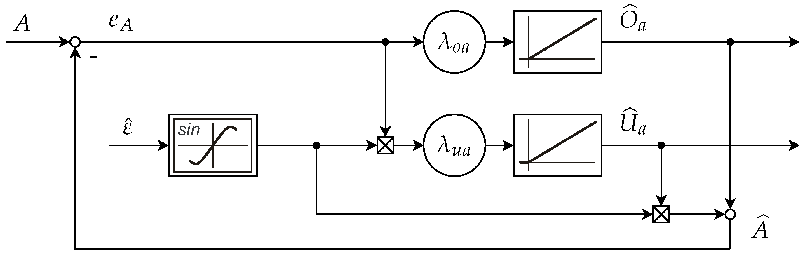
The structure of the observer is identical for both line signals with the only difference in the trigonometric function sine, respectively, cosine used. In the following, the approach is exemplarily explained for the line signal A, as shown in Figure 4. As can be seen from Figure 2, there is a feedback path for the estimated angle . The observer takes this signal and calculates the estimated erroneous signal by applying the offset and amplitude that was previously adapted. In a negative feedback loop internal to the observer, is then subtracted from the input A to obtain the error , which can be seen as the innovation to be used in the adaptation process:
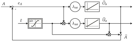
Figure 4.
Scheme of the observer for the line signal A.
The speed of the adaptation is defined by the learning rates and for total amplitude and offset. The offset parameter is determined by the integration of the error signal specified in (10).
This signal flow is in the upper part of Figure 4.
The amplitude parameter is gained by first multiplying the error with the ideal shape of the line signal and then scaled by the learning factor and integrating. In this way, the speed and sign of the parameter adaptation is directed towards the parameter that has the biggest effect to diminish the error signal at the current angular position. Assuming a constant offset and amplitude for both line signals, the four error parameters will converge towards the correct true values, if the adaptation runs over an extended period of time and over a range of angular positions that cover more than one cycle period of the encoder. If the integration runs over some time during which there is standstill of the encoder, the parameters of the error model will also converge to constant values, but not necessarily the correct ones. However, due to an internal negative feedback loop of the observer, there will be no instability and runaway of the parameters. If the standstill occurs after an already correct adaptation of the parameters, there will be no change of their values because then the error signal stays zero. Even if the parameters converged to false values in a standstill, the adaptation will continue in the right direction once the motion restarts. The parameter adaptation in the nonlinear observer can also be interpreted as a correlation of the error signal ( respective ) with the base function associated with the error parameter, 1 for offsets and sine or cosine for amplitude.
3.2. Stability
Stability can be investigated by the Ljapunov method [14]. The problem can be simplified by substituting the true mechanical angle ε for the estimated angle , which is used in the method. This assumption seems to be justified, if the offset and amplitude errors are in the range of only a few percent of the nominal value of the line signal amplitude. The proof of stability in this case can be referred to only one line signal because there is no cross coupling between the two line signals, if the true angle ε is used to reconstruct the distorted line signals. Thus, line A was chosen in this case. The reasoning can be translated for line B. The parameter difference between the true and estimated parameters is defined in (11) as vector . It is the state vector of the observer, represented by the two integrators in Figure 4. The according base functions (1 for offset, sine for amplitude) are written in (12) as vector .
The Ljapunov function is defined in Label (13). The desired point of convergence at the true parameter values is the equilibrium point , where the derivative of the parameters vanishes and the Ljapunov function becomes 0. For this purpose, the derivation of V to time t has to be less than or equal to 0. To prove this requirement in Label (14), the time derivative of the parameter difference and the gradient of V has to be determined. The derivative of can be taken from the inputs of the integrators in Figure 4, assuming both learning rates to be the same λ giving . The gradient evaluates to . If is set equal to ε, the product of the two vectors evaluates to Label (15). This means that is less than or equal to zero, as long as the learning rates are chosen to be positive. The other preconditions for Ljapunov stability, that the Ljapunov function is equal to zero at the equilibrium point itself and the Ljapunov function is greater than zero elsewhere, are also fulfilled. In summary, the Ljapunov stability is proved if the estimated angle is equal to the real angle. However, this does not include asymptotic convergence to the equilibrium point.
In a similar manner, the Ljapunov stability of the line signal B is verifiable:
The above equations show that the observer for the parameter offset and amplitude is stable, if the true angle is used in the adaptation. Because is negative semi definite, asymptotic stability is not proven. In simulation, we saw that the parameters indeed do not converge to the true values in standstill of the encoder. Only during motion can quick convergence within a few cycles of the line signals be achieved, if the learning rates are chosen appropriately in relation to the speed of rotation, and the true error parameters are constant. These convergence properties also hold, if the estimated angle is used in the observer to reconstruct the shape and offset of the line signals, as was shown in simulation. Obviously, the speed of the parameter convergence can be influenced by the learning rates , , and for each parameter. For small learning rates, the parameters converge slowly. In contrast, high learning rates lead to instability of the estimation and thereby an incorrect determination of the mechanical angle if the estimated angle is used in the observer. Figure 5 shows some oscillations with the frequency of the line cycle during transients of the offset error parameter. Higher learning rates would also result in increased oscillations. Additional selectable parameters are the initial values of the integrators. Large differences between the real parameter and the initial value can also cause instability of the estimation in this case. A good practical choice is to start with nominal values for all parameters, i.e., an initial value of 0 for the offset error estimation and an initial value of 1 for the total amplitude parameter because the true values should be close to these.
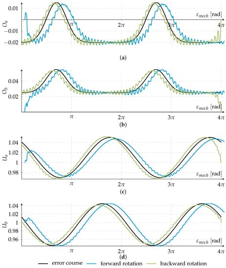
Figure 5.
Simulation results for parameter variation over one revolution of (a) the offset of line A; (b) offset of line B; (c) amplitude of line A and (d) amplitude of line B (32 line cycles per revolution).
With the limitations of well selected learning rates and initial values of the integrators, as well as relatively small errors on the line signals, the proposed method estimates the erroneous parameters of the line signals and correctly determines the true angle ε after the error correction of the line signals, if the error model matches the conditions in the encoder. Therefore, the proposed method does not need the true angle ε in the observer to estimate the offset and amplitude errors.
3.3. Simulation
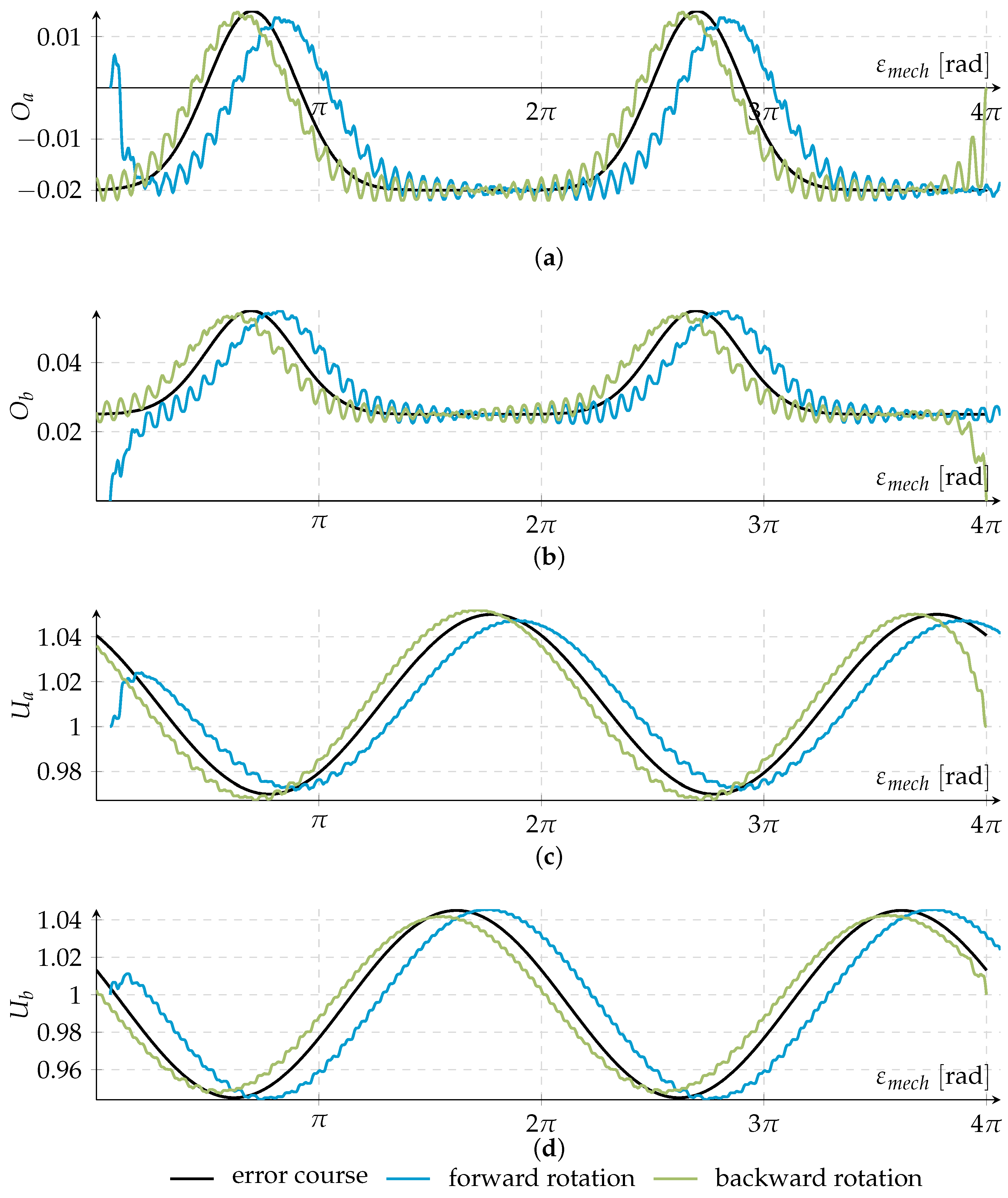
Up to this point, the true parameters of the error model () were assumed to be constant over time and independent of the mechanical rotation. Running a simulation with constant parameters shows that quick convergence within a few cycles of the encoder can be accomplished. At high learning rates, a convergence to values very close to the true error parameters were possible even within one cycle. However, measurements on different real encoders showed that the assumption of constant parameters for offset and amplitude does not hold. Instead, there is a variation over the mechanical revolution due to eccentricity of the optical disk, lithographic errors or other mechanical imperfections, such as variations of the distance between disk and optical system. Thus, the proposed method was tested in simulation for offset and amplitude errors that vary over one mechanical revolution but not between revolutions. For simulation, a scenario was set up to mimic this behavior. The disk was chosen with a low number of only 32 cycles. The courses of parameters of the error model consist of a constant part and a smooth variation dependent on the mechanical angle. The amplitude of the line signals varies sinusoidally over one mechanical revolution with an additional offset. The offset parameters are implemented as a Gaussian curve with an additional offset. The peak to peak variation of all four model parameters was chosen in a range of 5% of the nominal amplitude of the line signals because this seemed reasonable.
Figure 5 shows the simulation results of all error parameters over two revolutions for a forward and backward rotation at a speed of . The mechanical angle starts at 0 and increases to for the forward rotation and decreases from to 0 for the backward rotation. The black line ( ) represents the chosen error curve for each parameter. The blue ( ) and the green curve (  ) depict the estimated parameter course if the encoder turns forward or backward.
) represents the chosen error curve for each parameter. The blue ( ) and the green curve ( ) depict the estimated parameter course if the encoder turns forward or backward.Due to the method of estimation, the parameter curves are afflicted by high frequency oscillations depending on the line cycle frequency and ratio between learning rate and rotational speed. Another characteristic of this method is that the estimation is always delayed with respect to the direction of motion against the true error curve. This also results from the estimation procedure in the proposed design. The integrators need time to adjust to the correct value. Thus, there is a transient at the beginning of the estimation. This is shown at small angles for the forward rotation and in the range of for the backward rotation. Nevertheless, the overall shapes of the error parameter curves reproduced quite nicely. It must be noted that the proposed error model was originally set up to identify constant parameter values, but, in this case, the factors for the learning rate were driven up so high that the error parameters could even track time varying parameters.
3.4. Experimental Results
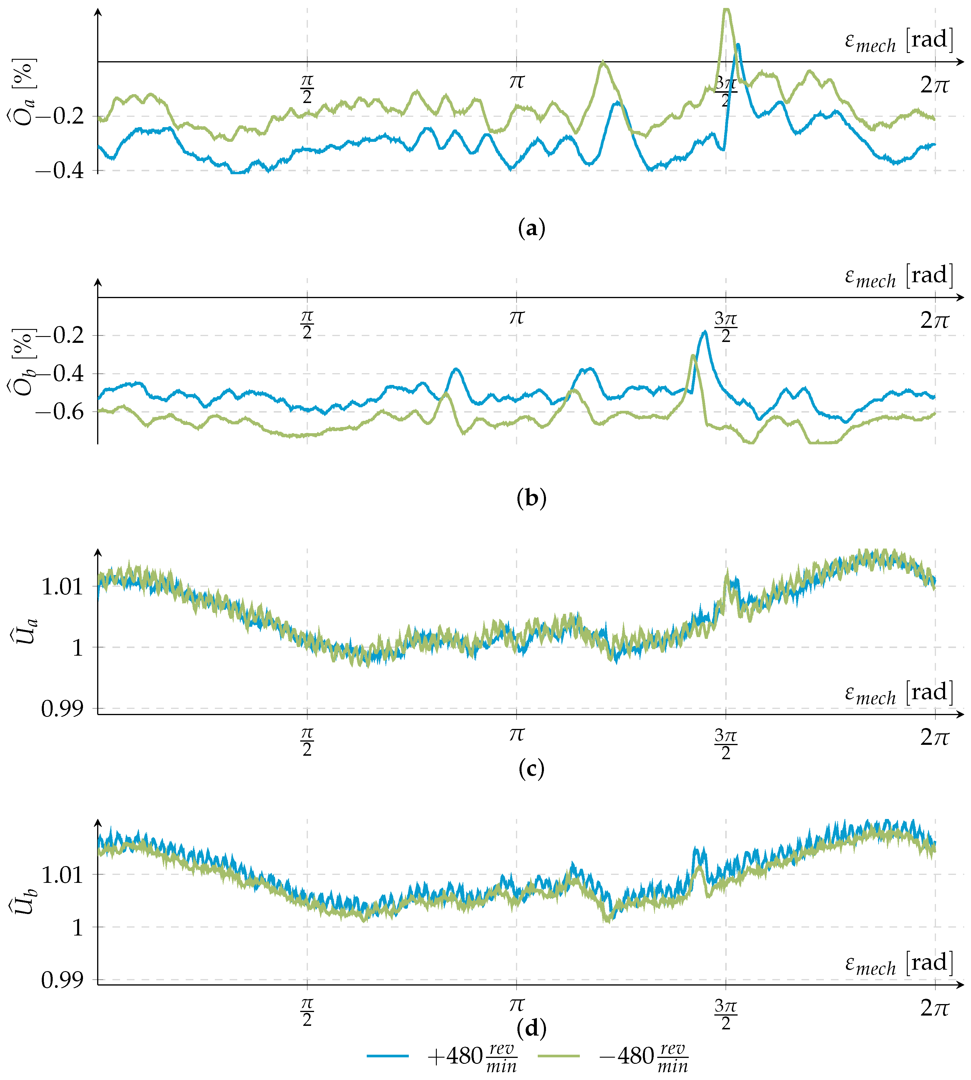
First, experimental results were able to confirm the behavior of the HEC method. The experimental setup is part of a general motor test bench with a PMSM motor and attached encoder with 2048 lines per revolution. The encoder line signals are prepared for digitalization with a two-stage amplifier circuit to match the ADC input voltage range. The amplified signals are simultaneously sampled by 14-bit ADCs at a sampling rate of 10 MHz. Sampled data is processed by an FPGA, performing the atan2(y,x) calculation and signal correction. The signal correction algorithm takes 5 s to evaluate, which equals an update rate of correction factors of 200 kHz. For this measurement, the motor was driven at a constant speed of 480 rpm. Therefore, the frequency of the line signals was 16,384 kHz.
Figure 6 shows the estimated parameter courses for one mechanical revolution as a function of the mechanical angle . The first and the second panel (a) and (b) show the offset course, and panels (c) and (d) the amplitude course of the two lines A and B. There are two curves in each panel, which represent forward and backward rotation at the same speed. The amplitude is estimated in analog-to-digital converter increments and is then normalized to the mean of several measurements at different speeds. The calculated offset is also estimated in analog-to-digital converter increments and then normalized to the mean of the amplitude courses, and is shown in percent.
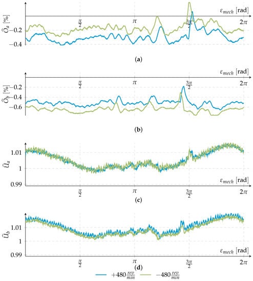
Figure 6.
Experimental results of the Harmonic Error Correction of (a) the offset of line A; (b) offset of line B; (c) amplitude of line A and (d) amplitude of line B (2048 line cycles per revolution).
The amplitude oscillates sinusoidally around the mean plus an offset as shown in Figure 6c,d. This could result from an eccentrically fixed encoder disk. The offset courses in Figure 6a,b are almost constant over one mechanical revolution with some characteristic peaks at certain points. It is striking that these peaks in curves A and B seem to be shifted by the same value. This could indicate that the sensors of lines A and B are displaced by this value and the optical disc has some lithographic manufacturing errors.
Striking is not only the shift between the A and B lines but also the shift within the same track depending on the direction of rotation. This is observable in each panel of Figure 6. This corresponds to the simulation results described in Section 3.3 and is a result of the estimation algorithm.
4. The Iterative Harmonic Error Correction
The proposed Iterative Harmonic Error Correction, IHEC, is an advancement of the Harmonic Error Correction described in Section 3. The disadvantages of the HEC method, a high-frequency oscillation on the estimated parameters during parameter transients and a lagging identification in direction of rotation, are eliminated.
The model of the HEC assumes that the error parameters are constant over time and mechanical revolution. Only a high learning rate allows fast tracking of the parameter course and direct use of this information to correct the line signals immediately at the following sampling step. If the model assumption of constant error parameters is substituted by an error parameter course as a function of the angular position, the integrated error can be stored in a table at the correct angular position, and the table entry be used as a precompensation for the next pass through the same angular position to accumulate residual parameter errors. This procedure is iterated over some revolutions until the absolute residual error drops below a predefined threshold.
4.1. Theoretical Structure
An overview of the scheme of the proposed IHEC is given in Figure 7 showing the basic signal flow. The measured line signals of the encoder are adjusted by the error correction depending on the estimated mechanical angle . The correction table contains the parameter course over one mechanical revolution depending on the mechanical angle . The table has been updated in previous revolutions or initialized to nominal values. Because the estimated value of the angular position is used to address the function values of the error parameters, this involves an algebraic loop, which has to be resolved by either an iteration or a delay by one sampling period. For simplicity, the latter was chosen with the assumption—that the angle difference between sampling steps is negligible. During every full revolution, the error parameters in the correction table will be updated by the observer output for use during the following revolution.

Figure 7.
Scheme of the proposed Iterative Harmonic Error Correction (IHEC).
The corrected line signals are used to compute the estimated angle of the line signals . It is important to distinguish between the angle of the line signals inside one optical cycle and the mechanical angle of the rotation , which covers a full mechanical rotation. The mechanical angle can be calculated from with the conversion block essentially counting overflows and underflows of at the transition between optical cycles of the encoder.
The main difference between IHEC and HEC lies in the fact that IHEC uses a filter window over equidistant samples of the mechanical angle with the exact length of one optical cycle. It operates as a finite impulse response (FIR) filter. Its filter coefficients are constant in the case of the two offset parameters (19) and (20) or contain the sine and cosine functions corresponding to their angular positions (21) and (22) within the optical cycle.
To determine the output of the observer and thus the estimated parameter course for one revolution, four calculation steps are required. These steps are repeated every revolution iteratively until the error signal is smaller than a defined limit. In the first step, the error signals between the corrected line signals , and the ideal line signals without offset and with the ideal amplitude of 1, are calculated based on the estimated angle (16):
In the second step, the error signals are sampled at equidistant angular positions and fed into an FIR filter whose length (angular samples) covers one line cycle of the encoder with a number of samples . Each error parameter in has its own FIR filter. These filters have different coefficients depending on the parameter to be estimated. In the third step, the FIR filter output is divided by the filter length , and this quotient is spread over the last table entries. In summary, operations two and three, to determine the modification of a parameter at one sampling point as represented by (17), are exemplarily shown for at sampling point n. By utilizing this operation, the high-frequency oscillations on the estimated parameters and a lagging identification, which are the disadvantages of the HEC method, are eliminated:
The new parameter course is determined in step four by adding the modification of a parameter to the old value of the last revolution r, shown in (18):
The filter coefficients for the FIR filters are chosen in the same way as in the HEC method at the respective angular positions. For the estimation of the offset error and , the filter coefficient is defined as the learning rate divided by the filter length , Equations (19) and (20). This corresponds to a simple moving average calculation. The filter coefficients for the amplitude parameters and also incorporate the learning rate divided by the filter length but additionally multiplied by a scaling factor and by the sine, respectively the cosine of the estimated angle at the considered point, Equations (21) and (22), to achieve the same behavior as in the HEC method:
The simulation of the IHEC method was run repetitively over three mechanical revolutions, which are completely shown in Figure 8. For a closed solution, the values of the error signals e outside the observation period have to be defined. In this case, they are set to zero. This results in a ramp-shaped slope at the left and right end of the estimated parameter courses for the IHEC method. The middle revolution from to does not show this effect.
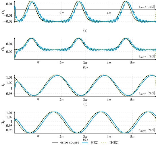
Figure 8.
Simulation results for parameter variation over one revolution of (a) the offset of line A; (b) offset of line B; (c) amplitude of line A and (d) amplitude of line B of both estimation methods.
As already described in Section 3.1, for the HEC method, it is necessary to have well defined initial values and learning rates. For the IHEC, the parameter courses for the initial revolution have to be defined. A good choice is an initial value of 0 for the offset error estimation and an initial value of 1 for the amplitude parameter estimation for a whole mechanical revolution. In addition, the number of iterations or a lower bound for the change of the parameter curves has to be chosen. With a skillful choice of the learning rates, the number of iterations can be kept low. The smaller the learning rates, the more iterations are necessary to estimate the real parameter curve. However, higher learning rates could cause an overshoot or even instability of the estimation.
4.2. Comparison
To compare the Harmonic Error Correction and the Iterative Harmonic Error Correction proposed in Section 3 and Section 4, both methods are simulated with the same erroneous line signals as inputs. The chosen line signals have the same course as before in Section 3.3. Figure 8 depicts the parameter courses for a simulation of three mechanical revolutions. The black line ( ) shows the erroneous parameter course, the blue line ( ) the estimated course obtained by the HEC and the dotted green line (  ) the same by IHEC, which is depicted after six iterations. As described in Section 4.1, the courses of the IHEC increase ramp-shaped at the right and left end of the estimation, but in the center part of the graphic, the curves track the chosen parameter course. Moreover, it must be noted that this performance is achieved after just a few iterations.
) shows the erroneous parameter course, the blue line ( ) the estimated course obtained by the HEC and the dotted green line ( ) the same by IHEC, which is depicted after six iterations. As described in Section 4.1, the courses of the IHEC increase ramp-shaped at the right and left end of the estimation, but in the center part of the graphic, the curves track the chosen parameter course. Moreover, it must be noted that this performance is achieved after just a few iterations.A clear difference between the IHEC and HEC is that the IHEC does not show high-frequency oscillations on the parameter courses mainly on the offsets, where frequency of the line cycle couples into the parameter adaption due to high learning rates. It shows very dominantly on the offset signals. Secondly, the simulation of both methods shows that the HEC compared to IHEC has an angle-shifted parameter identification delayed in the direction of rotation. Except for the IHEC, a few iterations are necessary for the error parameters to converge, always under the assumption that the course of the error parameters does not change between revolutions. This condition can be dropped with the HEC method.
Figure 9 depicts the difference between the true angle ε and the estimated angle in the simulation for both methods and without any error correction. The black line ( ) shows the angle difference, if the angle is determined without correcting the erroneous line signals. The blue ( ) and the green line ( ) show the difference if the HEC and the IHEC is applied. The improvement by the two correction methods is obvious. The IHEC provides the best compensation at the price, and several revolutions are needed to adapt to the error course.
) shows the angle difference, if the angle is determined without correcting the erroneous line signals. The blue ( ) and the green line ( ) show the difference if the HEC and the IHEC is applied. The improvement by the two correction methods is obvious. The IHEC provides the best compensation at the price, and several revolutions are needed to adapt to the error course.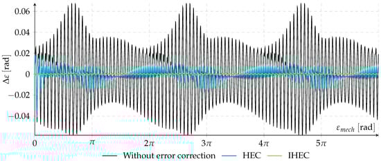
Figure 9.
Simulation results of the difference between the real and the estimated angle.
As both methods are based on different error models, the application depends on what types of errors are to be compensated. If we are to deal only with unsymmetrical photo diodes for positive and negative signs or between the lines, the parameter offset and amplitude will not be dependent on the mechanical rotation of the disk, and, therefore, an error model with constant parameters is adequate. Thus, the best choice is HEC. If errors from the etching process of the disk also play a mayor role, a table compensation with IHEC dependent on the mechanical angle is necessary. Of course, the implementation and calculation burden is much more complex for the IHEC. This was also the reason why this method was only investigated in simulation up to now. In summary, both methods are useful to estimate the errors on the sinusoidal line signals.
5. Conclusions
Encoders are widely used in motor drives to determine the mechanical angle of the motor shaft. Systematic errors of the resulting line signals are finally not preventable and affect the accuracy of the measured angle. Methods presented in this paper are able to identify amplitude and offset errors on the line signals and correct these to receive a more precise measured angle even without knowledge of a reference value for the mechanical angle during estimation. The error parameters may be constant or may depend on the mechanical angle. Both methods have been tested in simulation and have shown good to excellent convergence to the true error parameters. The HEC was also evaluated experimentally, confirming the results from simulation. To validate the Iterative Harmonic Error Correction, experimental studies are planned for this method.
The proposed methods are applicable to different requirements and have the presented advantages and disadvantages. The IHEC is practicable for angle-dependent errors, which are repetitive every revolution. In these application cases, an accurate estimation of the error courses is possible after a few iterations. The HEC estimates the error parameter continuously so there are no requirements on the type of the error. However, using the HEC leads to a lag of the estimation.
It is important to note that both methods use only the estimated angle to determine the error parameters, correct the line signals with these parameters in a feedback loop and compute the adjusted angle. In future research, a theoretical analysis of the stability limit of the estimation will be done. In addition, it could be useful to define criteria for the optimal values of the learning rates. As an extension of both models, the phase-shift between both line signals will also be taken into account in further studies. The IHEC method needs additional work for the practical implementation at arbitrary rotation speeds of the encoder because, during the first simulation tests reported here, an integer multiple of the line signal frequency was assumed for the sampling frequency of the angle discrete signal processing. In this way, re-sampling the time equidistant samples to obtain an integer number of samples in a line cycle, and, therefore, also in a mechanical revolution, was avoided.
Acknowledgments
The research was carried out by regular staff of Technische Universität Braunschweig.
Author Contributions
Jan Klöck conceived and designed the Harmonic Error Correction; Onno Martens performed the experiments; Walter Schumacher conceived and designed the Iterative Harmonic Error Correction; Carla Albrecht analyzed and simulated the Iterative Harmonic Error Correction; and Carla Albrecht wrote the paper.
Conflicts of Interest
The authors declare no conflict of interest.
Abbreviations
The following abbreviations are used in this manuscript:
| HEC | Harmonic Error Correction |
| IHEC | Iterative Harmonic Error Correction |
| ENDAT | Digital encoder communications protocol, proprietary Dr. Johannes Heidenhain GmbH |
| HIPERFACE® | Digital encoder communications protocol, proprietary SICK STEGMANN GmbH |
| BiSS | Open digital encoder communications protocol, iC-Haus GmbH |
| FPGA | Field Programmable Gate Array |
| HANN | Harmonic Activated Neural Network |
References
- EnDat 2.2—Bidirektionales Interface für Positionsmessgeräte. Technische Information company brochure from Dr. Johannes Heidenhain GmbH. Available online: http://www.endat.de (accessed on 19 December 2016).
- Specification Hiperface®: Motor Feedback Protocol. Company brochure from Sick Stegmann GmbH. Available online: https://www.sick.com (accessed on 19 December 2016).
- BiSS Interface. Protocol Description (C-Mode). Available online: http://biss-interface.com (accessed on 8 December 2016).
- Hwang, S.; Kim, D.; Kim, J.; Jang, D. Signal Compensation for Analog Rotor Position Errors due to Nonideal Sinusoidal Encoder Signals. J. Power Electron. 2014, 14, 82–91. [Google Scholar] [CrossRef]
- Gröling, C. Systematische Abweichungen auf dem Winkelistwert. Optimierungspotential bei Servoumrichtern für Permanenterregte Synchronmaschinen. Ph.D. Thesis, TU Braunschweig, Braunschweig, Germany, 2009; pp. 82–85. [Google Scholar]
- Höschler, B.; Számel, L. Innovative technique for easy high-resolution position acquisition with sinusoidal incremental encoders. In Proceedings of the PCIM Power Conversion & Intelligent Motion Conference, Nürnberg, Germany, 10–12 June 1997; pp. 407–415.
- Peterson, R. Quadrature Error Correction. U.S. Patent 5,134,404, 28 July 1992. [Google Scholar]
- Tan, K.; Tang, K. Adaptive Online Correction and Interpolation of Quadrature Encoder Signals Using Radial Basis Function. IEEE Trans. Control Syst. Technol. 2005, 13, 370–377. [Google Scholar]
- Kirchberger, R.; Hiller, B. Oversamplingverfahren zur Verbesserung der Erfassung von Lage und Drehzahl an elektrischen Antrieben mit inkrementellen Gebersystemen. In Proceedings of the SPS/IPC/Drives, Nürnberg, Germany, 23–25 November 1999; pp. 598–606.
- Daaboul, Y.; Schumacher, W. High-performance position evaluation for high speed drives via systematic error correction methods of optical encoders. In Proceedings of the 15th European Conference on Power Electronics and Applications (EPE), Lille, France, 2–6 September 2013.
- Bünte, A.; Beineke, S. High-Performance Speed Measurement by Suppression of Systematic Resolver and Encoder Errors. IEEE Trans. Ind. Electron. 2004, 51, 49–53. [Google Scholar] [CrossRef]
- Tan, K.; Zhou, H.; Lee, T. New Interpolation Method for Quadrature Encoder Signals. IEEE Trans. Instrum. Meas. 2002, 51, 1073–1079. [Google Scholar] [CrossRef]
- Schröder, D. Harmonisch Aktiviertes Neuronales Netz (HANN). In Intelligente Verfahren; Springer: Berlin, Germany, 2010; pp. 58–60. [Google Scholar]
- Adamy, J. Die Stabilitätstheorie von Ljapunov. In Nichtlineare Regelungstechnik; Springer: Berlin, Germany, 2009; pp. 95–99. [Google Scholar]


© 2017 by the authors. Licensee MDPI, Basel, Switzerland. This article is an open access article distributed under the terms and conditions of the Creative Commons Attribution (CC BY) license ( http://creativecommons.org/licenses/by/4.0/).