Initial Work on the Characterization of Additive Manufacturing (3D Printing) Using Software Image Analysis

Abstract

A current challenge in additive manufacturing (commonly known as 3D printing) is the detection of defects. Detection of defects (or the lack thereof) in bespoke industrial manufacturing may be safety critical and reduce or eliminate the need for testing of printed objects. In consumer and prototype printing, early defect detection may facilitate the printer taking corrective measures (or pausing printing and alerting a user), preventing the need to re-print objects after the compounding of a small error occurs. This paper considers one approach to defect detection. It characterizes the efficacy of using a multi-camera system and image processing software to assess printing progress (thus detecting completion failure defects) and quality. The potential applications and extrapolations of this type of a system are also discussed.

1. Introduction

Many additive manufacturing systems lack the capability to assess the quality of the products that they produce. Desktop 3D printers, for example, may continue printing until they have completed all steps in an object, even though their filament ran out or jammed part way through. These and other printers may fail to notice minor defects that could potentially be automatically corrected (if detected before another layer is deployed). They also cannot identify defects, which require manual intervention or may render the object unsuitable for use (necessitating the restarting of printing and rendering any additional time or supplies consumed on the current print wasteful).

When quality is critical, thus, it is necessary to test 3D printed objects post-production. However, this limits the type of objects that can be produced, as some tests may be destructive and, given the potential for irregularities in any item, testing a unit would not, for some applications, be suitable to certify a batch. Moreover, techniques like lean and just-in-time (JIT) manufacturing and total quality management (TQM) propose the use of process controls to eliminate acceptance and other testing costs. Given the forgoing, a mechanism for assessing quality of 3D printed items during production would seem to have the potential to offer significant benefit.

This paper considers one approach to performing quality assessment for 3D printed objects during the printing process. It utilizes digital imagery to assess the progress and quality of 3D printed objects. The efficacy of this assessment approach is considered and the potential uses for it are discussed.

2. Background

Several areas of prior work, which are relevant to the proposed characterization technique, are now reviewed. First, additive manufacturing is discussed. Next, 3D scanning technologies are reviewed. Finally, quality management is discussed.

2.1. Additive Manufacturing (3D Printing)

Three-dimensional printing, according to Berman [1], represents a “new industrial revolution”. It has the potential disrupt manufacturing in the way that online music and electronic books impacted their industries. The technology can be utilized for prototyping. It can also be utilized for short production runs and bespoke items. Examples include custom equipment parts, artificial limbs, dental fixtures and bridge components [1].

The 3D printing concept dates back to the 1970s [2]. The fused deposition modeling (FDM) technique [1] fuses layer of extruded material upon layer of extruded material to create an object. Laser sintering and power-based approaches have also been utilized [1] as has larger-scale printing using a rapidly setting masonry substance [3]. Biodegradable materials [4], imaging apertures [5], pharmaceuticals [6,7], nanocomposites [8], and microfluids [9] have all been 3D printed. The technology has been used for preserving and increasing access to historical objects (via replication) [10] and creating educational excitement [11].

Possible drawbacks for the technology also exist. Some have raised concern about the emissions from the printers [12]. Others have considered their prospective impact on society [13]. However, most relevant to this paper, is the concern that 3D printers cannot detect product defects, making them unsuitable for the production of safety-critical parts (or requiring a validation plan to be created for the item) [14].

2.2. Three-Dimensional Scanning

Three-dimensional scanning represents one approach to prospectively identifying defects in objects. The technology has been used to create custom running shoes [15], evaluate the impact of cosmetic products [16], size uniforms [17], and create custom swimwear [18]. It has also been used to detect a variety of changes and defects including changes in skeletal structure [19], validate the quality of automotive products [20] and to assess concrete [21] and turbine blades [22]. Approaches based on lasers have been demonstrated as have so-called “white light” techniques. Low-cost solutions using the Xbox Kinect [23] and Raspberry Pi cameras [24] have been created. Some scanners require scanner movement around an object [25,26]; others allow the object to remain stationary. The combination of projected light and camera sensing has also been proposed [27].

2.3. Quality Management

A complete discussion of quality management is far beyond the scope of this section. However, one point bears significant consideration in the context of the current work. This is the fact that some quality management systems, such as total quality management (TQM) [28], are highly reliant on suppliers being able to characterize and guarantee the quality of their parts. While this can be performed via inspection (either by the supplier, prior to shipping, or the buyer, upon receipt), process certification is preferred, as it can have reduced cost levels (via removing or reducing inspection time costs). Additionally, catching errors early in the production process reduces additional waste from more time and supplies being spent on a defective part. For 3D printed parts to be used under such a system they either need a more robust process control, such as Aron [14] discusses the lack of or extensive (and prospectively expensive) inspection.

2.4. Use of Imaging in Quality Assessment

Imaging and image processing has been used extensively for quality assessment. Fang, et al. [29], for example, discuss the use of imaging and a so-called “process signature” to identify defects in the process of the creation of a ceramic object using a fused deposition technique. Cheng and Jafari [30] also use imaging and image processing to detect defects in layered manufacturing. Their approach uses a control-feedback approach and follows the so-called “road path” (the path taken when depositing material) to identify over- and under-fill conditions. This approach appears to be comparatively computationally intensive (based on applying a fuzzy model) and is limited to the identification and characterization of a single type of defect. Szkilnyk, Hughes, and Surgenor [31] also used image processing for quality assessment, in this case in a manufacturing assembly environment. They found that the imaging/image processing system could detect defects (such as jams), but only those that were known a priori.

Nandi, Tudu, and Koley [32], and Lee, Archibald, and Xiong [33] look at the efficacy of using a vision system for assessing the maturity level and other quality aspects of fruits via the assessment of their color. A sub-field of image processing, known as structured light techniques, has also been utilized in quality assessment. Structured light approaches can be used to obtain 3D measurements [34] (and the approach has been used to make 3D scanning systems [35]), to determine range-to-object [36] and to characterize surfaces (by comparing a projected and sensed pattern) [37,38]. Structure light techniques have, for example, been used to monitor the fermentation of bread dough [39], which has been shown to correlate with the bread’s internal structure [40] and bread quality.

3. Research Methods and Experimental Design

The goal of the experiment described in this article was to test the hypothesis that image processing could be utilized to characterize differences in 3D printed objects. To this end, a system for imaging objects during the printing process was required. An experimental setup was created using a MakerBot Replicator 2 3D printer and five camera units. The camera units were comprised of a Raspberry Pi and Raspberry Pi camera and were networked using Ethernet cable and a switch to a central server which triggered imaging. These cameras were configured and controlled in the same manner as used for the larger-size 3D scanner described in [24].

The cameras were positioned around the 3D printer, as shown in Figure 1 and placed on stands comprised of a 3D printed base and a polyvinyl chloride (PVC) pipe. These stands were affixed to the table utilizing double-sided tape. Three different views of a CAD model depicting the stands, printer and their relative placement are presented in Figure 1a–c.

Figure 1. CAD renderings of system from (a) top; (b) side-angle and (c) front.

Figure 1. CAD renderings of system from (a) top; (b) side-angle and (c) front.

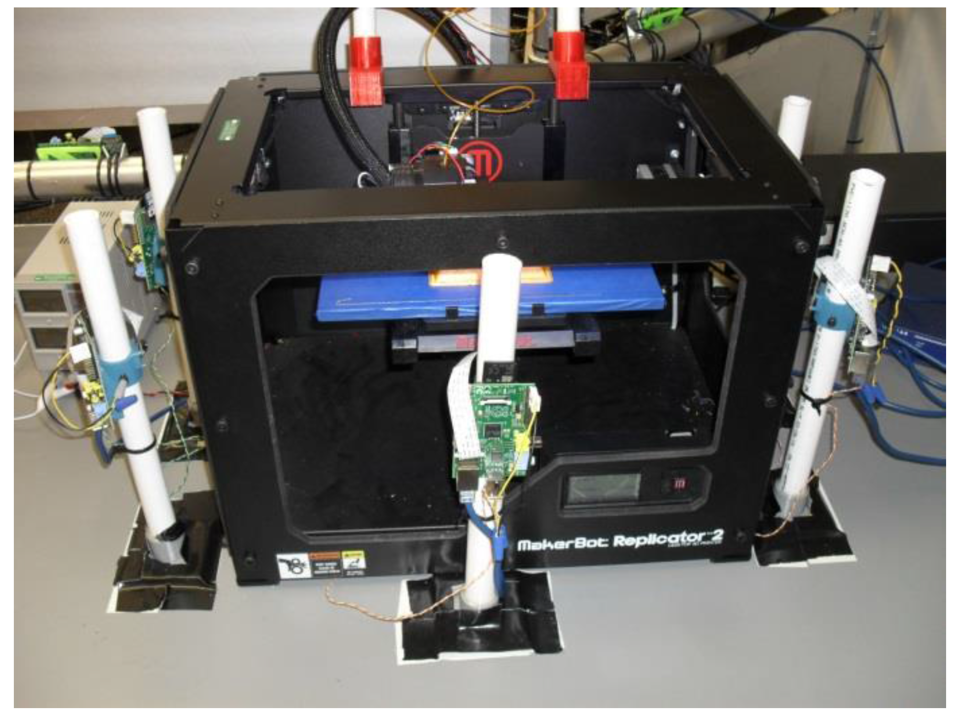
An Ethernet cable and power cable were run to each camera. The power cables were connected to a variable DC power supply (shown in the far left of Figure 2). The Ethernet cables were connected to a server via a switch. Imaging is triggered from the server’s console, avoiding the inadvertent imaging of researchers.

Figure 2. Image of experimental setup.

Figure 2. Image of experimental setup.

To facilitate comparison, it was desirable to have the images taken at a single 3D printer configuration. This would reduce the level of irrelevant data in the image from non-printed-object changes (in a system taking images continuously and not at a rest position, position changes as well as operating vibration would introduce discrepancies that would need to be corrected for). Data was collected by stopping the printing process at numerous points and placing the printer in sleep mode, which moved the printing plate to a common position. It was believed that this was the same position as the printer returns to when a job is complete; unfortunately, this was found to be inaccurate (as this final position is a slightly lower level. For this reason, the image that was supposed to serve as the final in-process image (in which the structure is very nearly done) has been used as the target object for comparison purposes. Image data from eight positions from each of five angles (for a total of 40 images) was thus collected and analyzed using custom-developed software created using C# and the Dot Net Framework for comparing images and generating the results presented in the subsequent section.

It is important to note that no action was taken to exclude factors, which could introduce noise into the data. For example, panels could have been installed around the scanner or another method for blocking changes outside of the scanner could have been implemented. Modifications could also have been made to aspects of the scanner itself (such as covering logos) to make it more consistent (and less likely to cause confusion with the orange colored filament); however, in both cases, this would have impaired the assessment of the operation of this approach in real world conditions.

4. Data Collected

Data analysis involved a comparison of the in-process object to the final object. Note that, in addition to the obvious application of characterizing build progress, this comparison could prospectively detect two types of potential error: when a build has been stopped mid-progress resulting in an incomplete object and when an issue with the printer results in a failure to dispense or deposit filament. 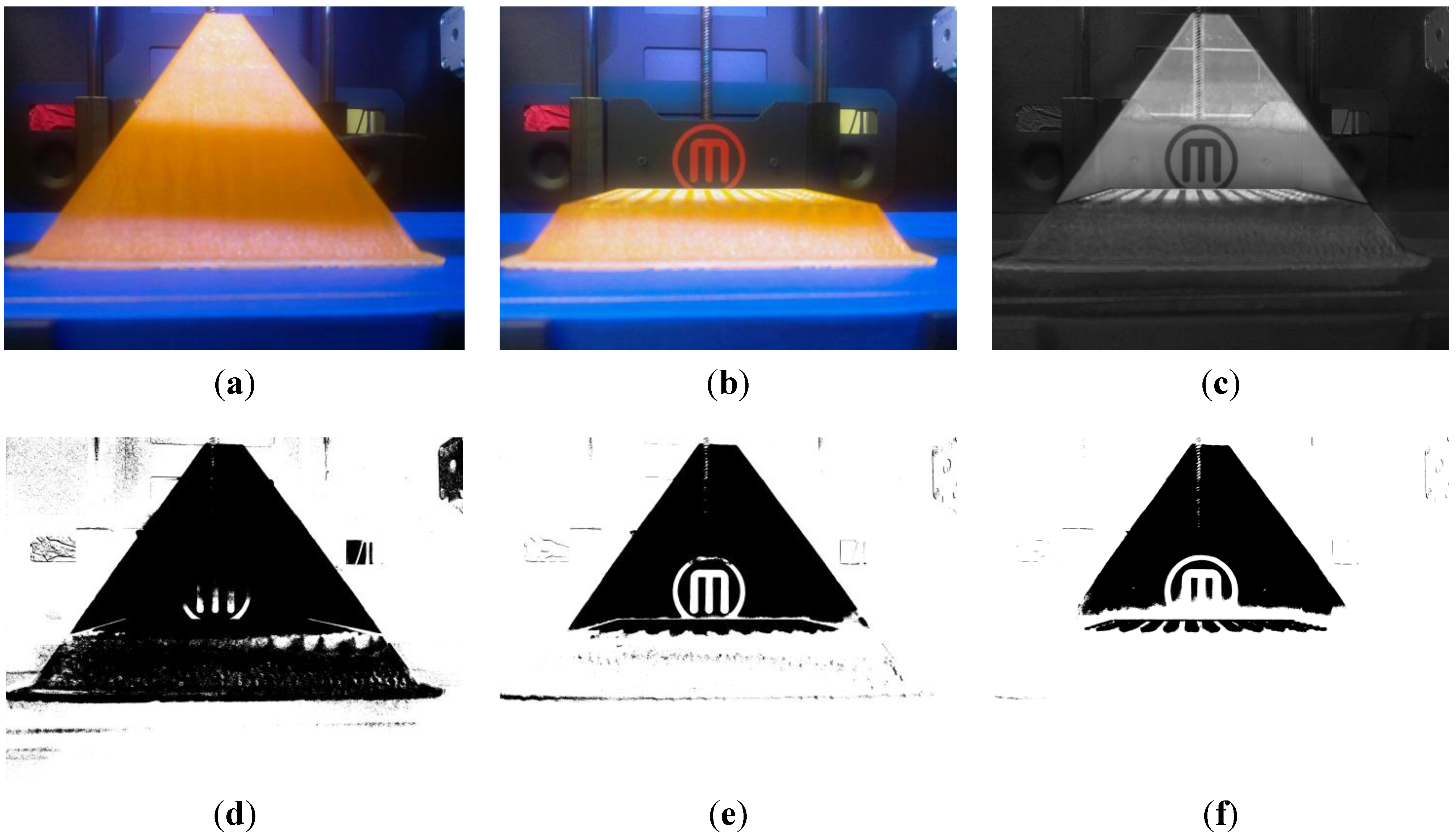Figure 3a shows the image (for the front camera position) that was used as the complete object and Figure 3b shows partial object from the first progress step.

The final and in-progress images are next compared on a pixel-by-pixel basis. The result of this comparison is the identification of differences between the two images. Figure 4c characterizes the level of difference in the image: brighter areas represent the greatest levels of difference. This image is created by placing, for each pixel, a brightness value (the same red, green and blue values), which correspond to a scaled level of difference. The scale factor is calculated via:

$$ScaleFactor=\frac{255}{MaxDifference}$$

(1)

MaxDifference is the maximum level of the summed difference of the red, green and blue values for any single pixel anywhere in the image. This is determined, for the pixel at position x = i, y = j, by calculating this summed difference:

$$Differenc{e}_{i,j}=Difference{R}_{i,j}+Difference{G}_{i,j}+Difference{B}_{i,j}$$

(2)

where MaxDifference is the largest value of Difference_i,j recorded for any position. Using this, the brightness value for the pixel at position x = i, y = j is computed using:

$$Brightnes{s}_{i,j}=Differenc{e}_{i,j}\times ScaleFactor$$

(3)

As is clear from Figure 3c, not all difference levels are salient. Areas outside of the pyramid area are not completely black (as they would be if there was absolutely no difference), but should not be considered. Thus, a threshold is utilized to determine salient levels of difference from presumably immaterial ones. Pixels exceeding this difference threshold are evaluated; those failing to exceed this value are ignored. Given the importance of this value, several prospective values were evaluated for this application. Figure 3d–f show the pixels included at threshold levels of 50, 75 and 100. In these images, the black areas are the significant ones and white areas are ignored.

Figure 3. Examination of various threshold levels: (a) complete object; (b) partially printed object; (c) showing difference between partial and complete object; (d) threshold of 50; (e) threshold of 75; (f) threshold of 100.

Figure 3. Examination of various threshold levels: (a) complete object; (b) partially printed object; (c) showing difference between partial and complete object; (d) threshold of 50; (e) threshold of 75; (f) threshold of 100.

In this particular example, a threshold level of 50 incorrectly selects the base of the object (which is the same as the final object) as different. The 75 threshold level correctly characterizes this base as the same, while (perhaps) detecting a slight pulling away of the object from the build plate (the indicated-significant area on the bottom left). It also (incorrectly) identifies a small area in the middle of the in-progress object and (correctly) the visible lattice from construction. A clear demarcation between the remainder of the object that hasn’t yet printed and the already printed area is also clear. The 100 threshold (incorrectly) ignores a small bottom area of this region. The MakerBot logo is not identified as a different, given the closeness of its red color to the orange filament.

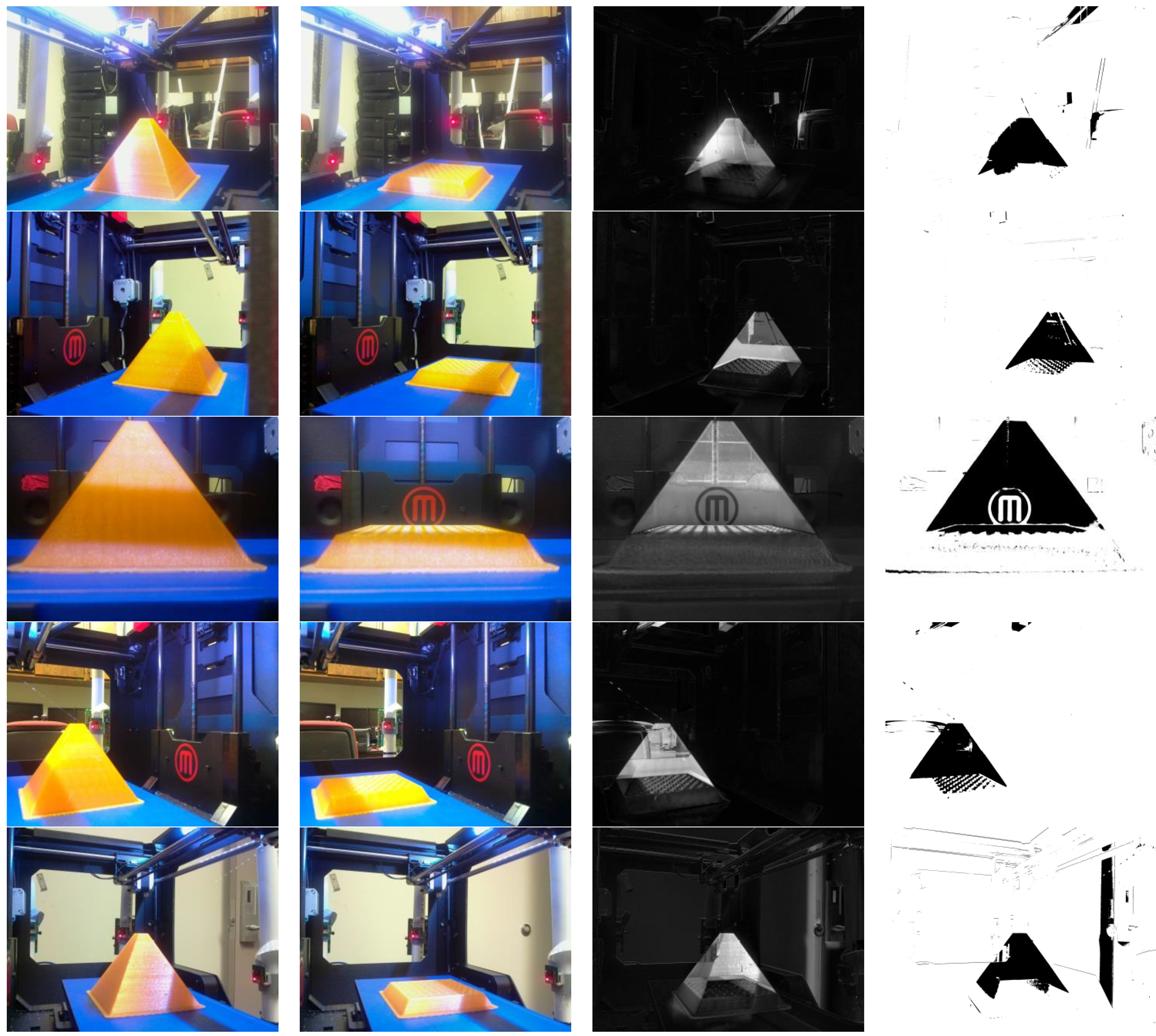
Given the results of this experiment, the 75 difference threshold level was selected for use going forward. This was applied to all of the images from all five cameras and eight progress levels. In Figure 5, the processing of the progress level 1 image for all five camera positions is shown. The leftmost column shows the finished object. The second column shows the current progress of printing of this object. The third and fourth columns characterize the areas of greatest difference (brightest white) from areas of less significant (darker) difference and the identification of pixels exceeding the difference threshold, respectively.

Figure 4. Images from all angles (at a 75 threshold level). The first column is the finished object image, the second column is the partial (stage 1) object. The third and fourth columns depict the partial-complete difference comparison and threshold-exceeding pixels identification.

Figure 4. Images from all angles (at a 75 threshold level). The first column is the finished object image, the second column is the partial (stage 1) object. The third and fourth columns depict the partial-complete difference comparison and threshold-exceeding pixels identification.

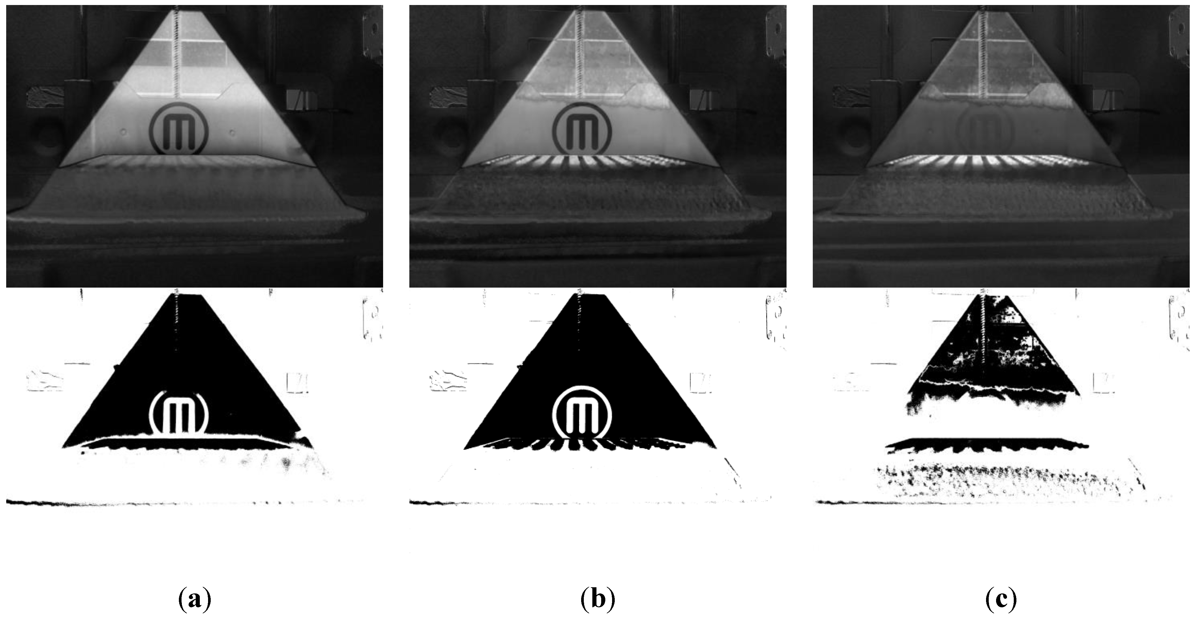
The impact of excluding the consideration of certain colors was, next considered. Figure 6 shows the impact of excluding the blue, green and red channels. Figure 5a shows the exclusion of blue and Figure 5b shows the exclusion of green. Neither exclusion corrects the MakerBot logo issue (though the blue exclusion creates greater difference levels around two indentations to either side of it). Excluding red has a significant impact on MakerBot logo; however, it places many different pixels below the significant pixel detection threshold.

Given that the total difference is a summed and not an averaged value, it makes sense to adjust the threshold when part of the difference level is excluded. Figure 7 shows the impact of manipulating the threshold value. Figure 6a shows a threshold value of 75, while Figure 6b,c show the impact of threshold values of 62 and 50, respectively.

Figure 5. Depicting the impact of excluding (a) blue; (b) green; and (c) red from the difference assessment. The top row depicts the partial-complete object difference and the bottom depicts the threshold-exceeding areas (using a 75 threshold level).

Figure 5. Depicting the impact of excluding (a) blue; (b) green; and (c) red from the difference assessment. The top row depicts the partial-complete object difference and the bottom depicts the threshold-exceeding areas (using a 75 threshold level).

Figure 6. Impact of excluding red at threshold levels of (a) 75; (b) 62; and (c) 50.

Figure 6. Impact of excluding red at threshold levels of (a) 75; (b) 62; and (c) 50.

As the MakerBot logo issue could be easily corrected via applying tape or paint over the logo (or through explicit pre-processing of the images), this was not considered further (and color exclusion is not used in subsequent experimentation, herein). However, it has been included in the discussion to demonstrate the efficacy of the technique for dealing with erroneously classified pixels. Additional manipulation of the threshold level (as well as a more specific color exclusion/inclusion approach) could potentially be useful in many applications.

Work now turned to detecting the level of completeness of the object (also relevant to assessing build progress). To this end, data from all eight progress levels was compared to the final image. The difference was depicted visually as well as assessed quantitatively.

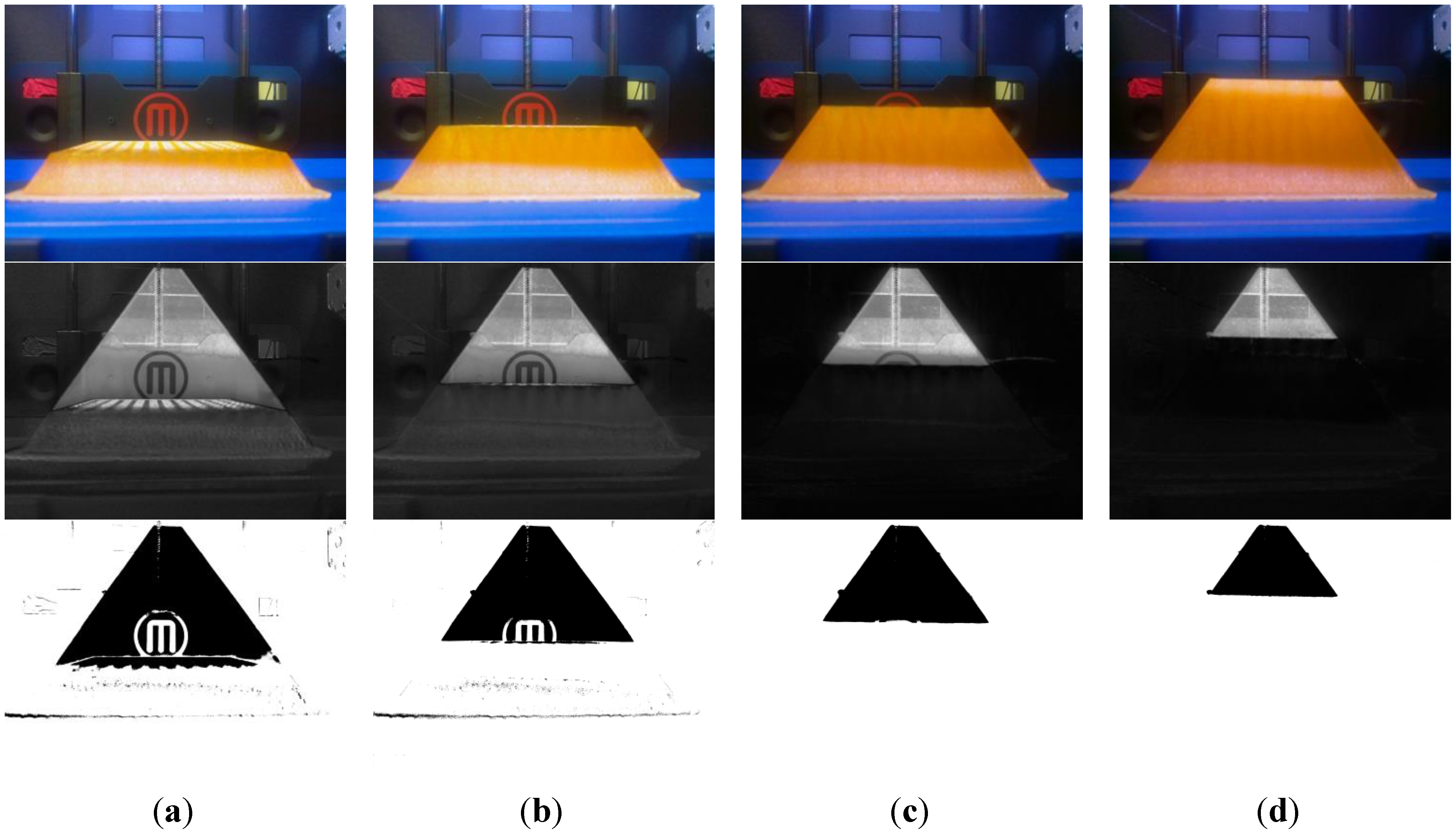
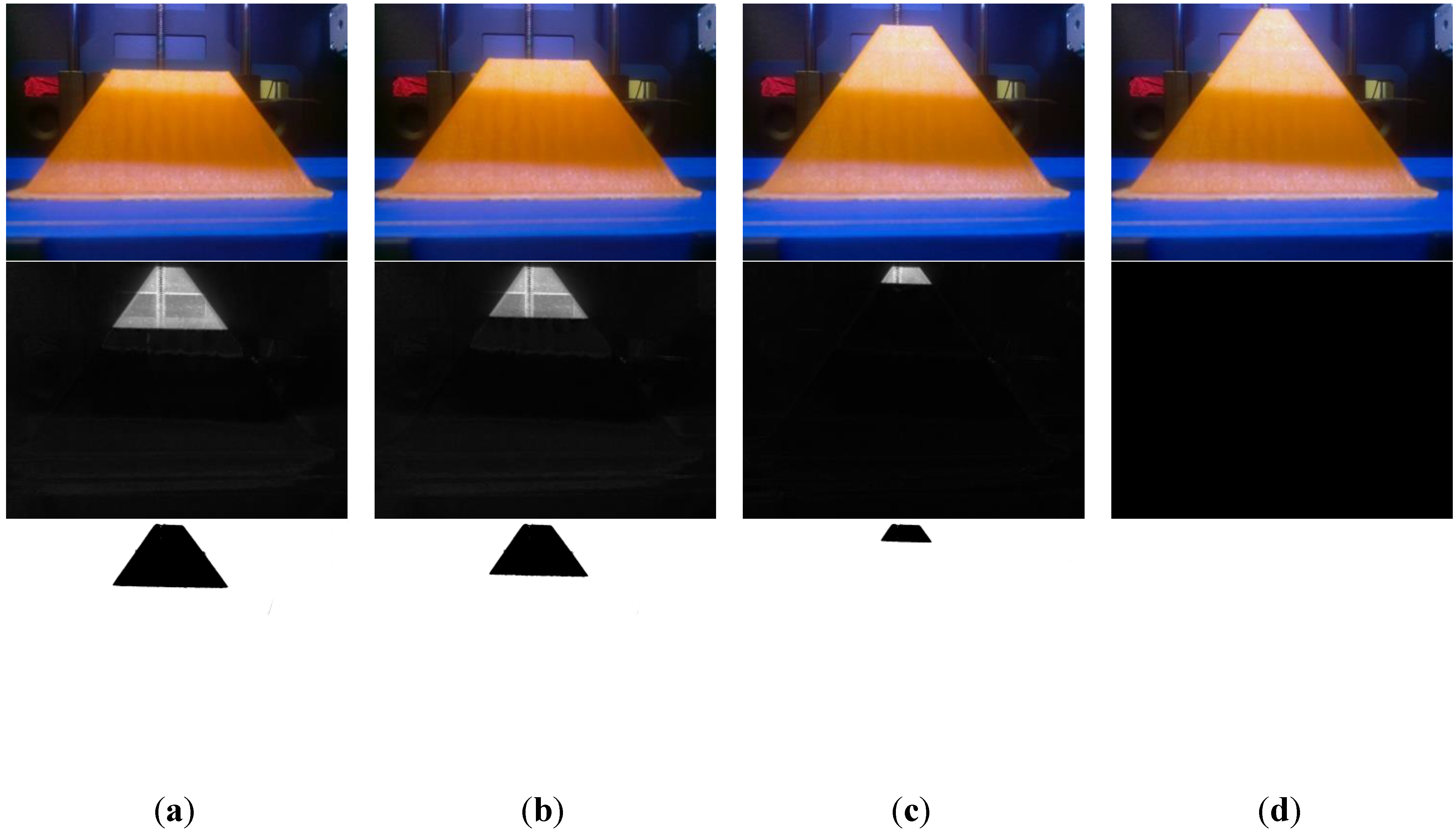
Figure 7 and Figure 8 present all eight progress levels for angle 3 (the front view). The top row shows the captured image. The second row displays the characterization of the difference level and the bottom row shows the pixels that are judged, via the use of the threshold, to be significantly different.

Figure 7. Progression of object through the printing process: (a) progress point 1; (b) progress point 2; (c) progress point 3; (d) progress point 4.

Figure 7. Progression of object through the printing process: (a) progress point 1; (b) progress point 2; (c) progress point 3; (d) progress point 4.

Figure 8. Progression of object through the printing process: (a) progress point 5; (b) progress point 6; (c) progress point 7; (d) progress point 8 (this is also used as the complete object).

Figure 8. Progression of object through the printing process: (a) progress point 5; (b) progress point 6; (c) progress point 7; (d) progress point 8 (this is also used as the complete object).

The build progress/object completeness is, thus, quite clear with a visible progression from Figure 7a to Figure 8d. It is also notable that some very minor background movement/movement relative to the background may have occurred between progress points two and three, resulting in the elimination of the limited points detected in the background in the third rows of Figure 7a,b.

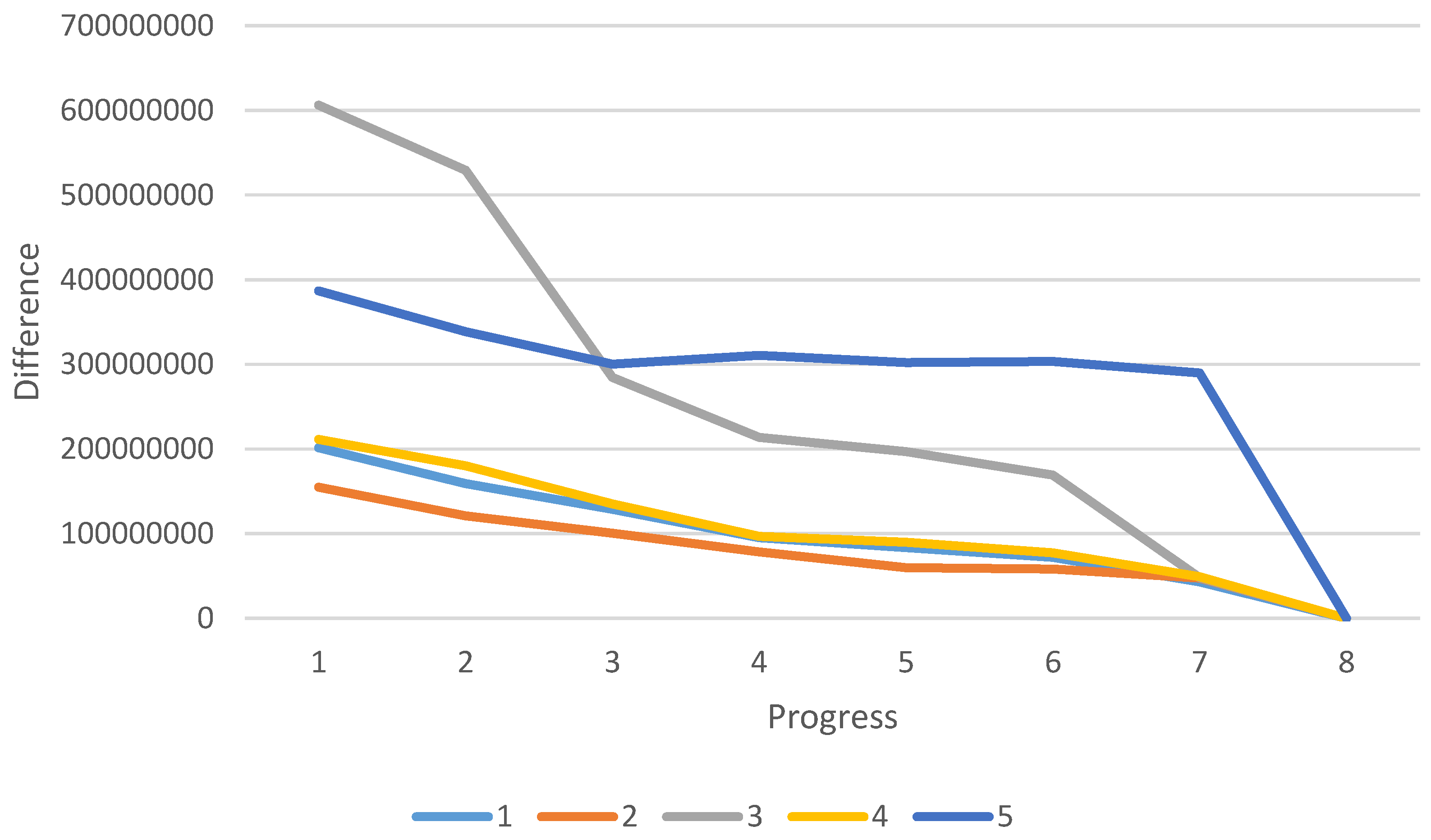
The quantitative data from this collection process is presented in Table 1 (and depicted visually in Figure 9), which shows the aggregate level of difference (calculated via summation of the difference levels of each pixel, using Equation (4)) by progress level and camera position.

$$AggregateDifference={\displaystyle \sum }_{i=\mathrm{0..}m,j=\mathrm{0..}n}Differenc{e}_{i,j}$$

(4)

where difference_i,j is the difference between values at pixel i, j and m and n are the maximum values for x and y. A clear progression of declining difference can also be seen in this numeric data.

Table 1. Aggregate difference by level of progress and angle.

		Angle
		1	2	3	4	5
Progress	1	201575263	154742364	606260772	211214209	386909779
	2	159074877	120966265	529193273	180098380	338718052
	3	128796927	100588139	284574631	135275350	300301392
	4	95224509	78451958	213765197	96921027	310651833
	5	83581787	59900209	196817866	89931596	302212892
	6	72126962	58127383	169154720	77356784	303391576
	7	43090774	47638489	48088649	49056229	289977798

Table 1. Aggregate difference by level of progress and angle.

		Angle
		1	2	3	4	5
Progress	1	201575263	154742364	606260772	211214209	386909779
	2	159074877	120966265	529193273	180098380	338718052
	3	128796927	100588139	284574631	135275350	300301392
	4	95224509	78451958	213765197	96921027	310651833
	5	83581787	59900209	196817866	89931596	302212892
	6	72126962	58127383	169154720	77356784	303391576
	7	43090774	47638489	48088649	49056229	289977798

Figure 9. Visual depiction of data from Table 1.

Figure 9. Visual depiction of data from Table 1.

Table 2 presents the maximum difference, which is calculated:

$$MaxDifference=Ma{x}_{i=\mathrm{0..}m,j=\mathrm{0..}n}\left(Differenc{e}_{i,j}\right)$$

(5)

where Max() is a function that selects the maximum value within the set of values from the proscribed range. While there is decline in maximum difference as the progress levels advance, the correlation is not absolute, as there are instances where the difference increases from a progress level to the next subsequent one.

Table 2. Maximum difference level by level of progress and angle.

		Angle
		1	2	3	4	5
Progress	1	633	568	542	604	669
	2	631	477	539	665	663
	3	613	489	584	661	648
	4	583	476	568	656	624
	5	562	485	559	658	625
	6	555	473	561	667	606
	7	502	435	446	609	564

Table 2. Maximum difference level by level of progress and angle.

		Angle
		1	2	3	4	5
Progress	1	633	568	542	604	669
	2	631	477	539	665	663
	3	613	489	584	661	648
	4	583	476	568	656	624
	5	562	485	559	658	625
	6	555	473	561	667	606
	7	502	435	446	609	564

Additional analysis of this data is presented in Table 3 and Table 4 which present the average level of difference for each progress level and angle and the percentage of difference relative to total difference, respectively. The aggregate difference (Table 1) and average difference (Table 3) for angle 3 are higher for most levels due to the fact that the object fills significantly more of the image area from this angle. Looking at the difference from a percentage perspective (in Table 4) demonstrates that the object completion values (ignoring the amount of image space covered) are much closer to the other angles. This is calculated via:

$$AvgDiff=Av{g}_{i=\mathrm{0..}m,j=\mathrm{0..}n}\left(Differenc{e}_{i,j}\right)$$

(6)

where Avg() is a function that returns the average for the set of values from the range provided. The average Table 4 percentage of distance values are calculated using:

$$PercentDiff=\frac{AvgDiff}{TotalDifference}$$

(7)

where TotalDifference is the summation of the difference at all of the progress levels.

Table 3. Average level of difference per-pixel by level of progress and angle.

		Angle
		1	2	3	4	5
Progress	1	40.00	30.71	120.32	41.92	76.79
	2	31.57	24.01	105.02	35.74	67.22
	3	25.56	19.96	56.48	26.85	59.60
	4	18.90	15.57	42.42	19.23	61.65
	5	16.59	11.89	39.06	17.85	59.98
	6	14.31	11.54	33.57	15.35	60.21
	7	8.55	9.45	9.54	9.74	57.55

Table 3. Average level of difference per-pixel by level of progress and angle.

		Angle
		1	2	3	4	5
Progress	1	40.00	30.71	120.32	41.92	76.79
	2	31.57	24.01	105.02	35.74	67.22
	3	25.56	19.96	56.48	26.85	59.60
	4	18.90	15.57	42.42	19.23	61.65
	5	16.59	11.89	39.06	17.85	59.98
	6	14.31	11.54	33.57	15.35	60.21
	7	8.55	9.45	9.54	9.74	57.55

Table 4. Percentage of difference by level of progress and angle.

		Angle
		1	2	3	4	5
Progress	1	25.7%	24.9%	29.6%	25.1%	17.3%
	2	20.3%	19.5%	25.8%	21.4%	15.2%
	3	16.4%	16.2%	13.9%	16.1%	13.5%
	4	12.2%	12.6%	10.4%	11.5%	13.9%
	5	10.7%	9.7%	9.6%	10.7%	13.5%
	6	9.2%	9.4%	8.3%	9.2%	13.6%
	7	5.5%	7.7%	2.3%	5.8%	13.0%

Table 4. Percentage of difference by level of progress and angle.

		Angle
		1	2	3	4	5
Progress	1	25.7%	24.9%	29.6%	25.1%	17.3%
	2	20.3%	19.5%	25.8%	21.4%	15.2%
	3	16.4%	16.2%	13.9%	16.1%	13.5%
	4	12.2%	12.6%	10.4%	11.5%	13.9%
	5	10.7%	9.7%	9.6%	10.7%	13.5%
	6	9.2%	9.4%	8.3%	9.2%	13.6%
	7	5.5%	7.7%	2.3%	5.8%	13.0%

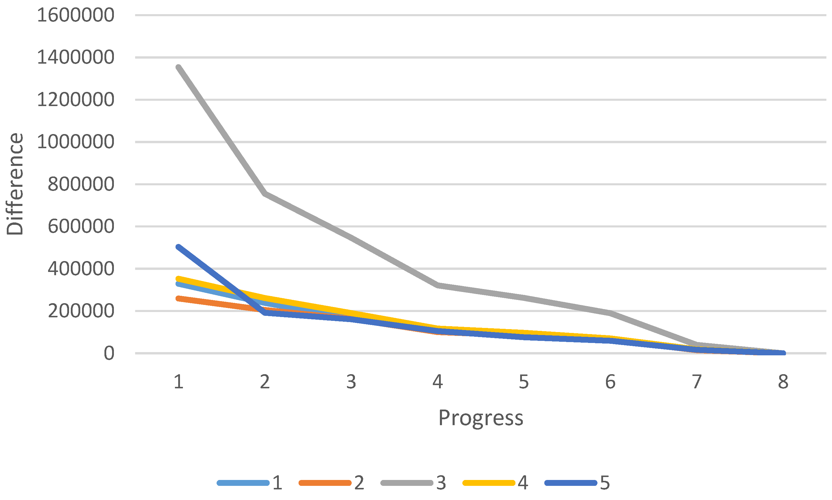
The aggregate difference level (and derivative metrics) provide one way to assess the completion; however, this is impacted by lots of small ambient differences as well as the level of difference between the final object and the background (which could be inconsistent across various areas of the object). An alternate approach is to simply count the number of pixels, which have been judged via the use of the threshold value, to be significantly different. This, particularly for cases where lighting changes occur or foreground-background differences are inconsistent, reduces the impact of non-object differences. Data for the number of pixels that are different is presented in Table 5. and visually depicted in Figure 10. This is calculated using:

$$NumDiffPix=Coun{t}_{i=\mathrm{0..}m,j=\mathrm{0..}n}\left(Differenc{e}_{i,j}>Thres\right)$$

(8)

where Count() is a function that determines the number of instances within the range provided where a condition is true. Thres is the specified threshold value used for comparison purposes.

One notable issue exists in this data. A slight movement of a door that falls within the viewing area of angle five occurred between progress points one and two, creating a significantly higher number of difference points in angle five, progress point one. This is a far more pronounced impact than this had on the aggregate difference approach (in Table 1). This type of movement could be excluded through greater color filtering and/or enclosing the printer in an opaque box or wrap.

Table 5. Number of pixels with above-threshold difference, by progress level and angle.

		Angle
		1	2	3	4	5
Progress	1	328775	258901	1353743	352334	503292
	2	238267	204661	755034	261407	191781
	3	166407	163139	545944	190409	161034
	4	108800	100143	321195	117178	105233
	5	94427	83715	261903	96687	75725
	6	68056	63622	189724	70255	59148
	7	15088	14094	39813	18292	16624

Table 5. Number of pixels with above-threshold difference, by progress level and angle.

		Angle
		1	2	3	4	5
Progress	1	328775	258901	1353743	352334	503292
	2	238267	204661	755034	261407	191781
	3	166407	163139	545944	190409	161034
	4	108800	100143	321195	117178	105233
	5	94427	83715	261903	96687	75725
	6	68056	63622	189724	70255	59148
	7	15088	14094	39813	18292	16624

The Table 6 percent of pixels value is determined using the equation:

$$PercentPix=\frac{NumDiffPix}{TotalPixelCount}$$

(9)

where the TotalPixelCount is determined by multiplying the m and n (maximum x and y) values.

Figure 10. Visual Depiction of Data from Table 5.

Figure 10. Visual Depiction of Data from Table 5.

Table 6. Percent of pixels with above-threshold difference, by progress level and angle.

		Angle
		1	2	3	4	5
Progress	1	6.52%	5.14%	26.87%	6.99%	9.99%
	2	4.73%	4.06%	14.98%	5.19%	3.81%
	3	3.30%	3.24%	10.83%	3.78%	3.20%
	4	2.16%	1.99%	6.37%	2.33%	2.09%
	5	1.87%	1.66%	5.20%	1.92%	1.50%
	6	1.35%	1.26%	3.77%	1.39%	1.17%
	7	0.30%	0.28%	0.79%	0.36%	0.33%

Table 6. Percent of pixels with above-threshold difference, by progress level and angle.

		Angle
		1	2	3	4	5
Progress	1	6.52%	5.14%	26.87%	6.99%	9.99%
	2	4.73%	4.06%	14.98%	5.19%	3.81%
	3	3.30%	3.24%	10.83%	3.78%	3.20%
	4	2.16%	1.99%	6.37%	2.33%	2.09%
	5	1.87%	1.66%	5.20%	1.92%	1.50%
	6	1.35%	1.26%	3.77%	1.39%	1.17%
	7	0.30%	0.28%	0.79%	0.36%	0.33%

Table 7 presents the percentage of difference, based on only considering difference values above the identified threshold. The Table 7 percentage of difference values are calculated via:

$$AggThresDiff=SumI{f}_{i=\mathrm{0..}m,j=\mathrm{0..}n}\left(Differenc{e}_{i,j},Differenc{e}_{i,j}>Thres\right)$$

(10)

where SumIf() is a function that sums the value provided in the first parameter, if the logical statement that is the second parameter evaluates to true.

Table 7. Percentage of difference at each level of progress and angle.

		Angle
		1	2	3	4	5
Progress	1	32.2%	29.1%	39.0%	31.8%	45.2%
	2	23.4%	23.0%	21.8%	23.6%	17.2%
	3	16.3%	18.4%	15.7%	17.2%	14.5%
	4	10.7%	11.3%	9.3%	10.6%	9.5%
	5	9.3%	9.4%	7.6%	8.7%	6.8%
	6	6.7%	7.2%	5.5%	6.3%	5.3%
	7	1.5%	1.6%	1.1%	1.7%	1.5%

Table 7. Percentage of difference at each level of progress and angle.

		Angle
		1	2	3	4	5
Progress	1	32.2%	29.1%	39.0%	31.8%	45.2%
	2	23.4%	23.0%	21.8%	23.6%	17.2%
	3	16.3%	18.4%	15.7%	17.2%	14.5%
	4	10.7%	11.3%	9.3%	10.6%	9.5%
	5	9.3%	9.4%	7.6%	8.7%	6.8%
	6	6.7%	7.2%	5.5%	6.3%	5.3%
	7	1.5%	1.6%	1.1%	1.7%	1.5%

In addition to looking at the raw number of pixels exhibiting difference, this can also be assessed as a percentage of pixels exhibiting a difference in the image (Table 6) or, more usefully, as the percentage of total difference level (Table 7). These values, again, show a consistent decline in difference from progress level to subsequent progress level.

5. Analysis of Data Collected

The data collected demonstrates a correlation between object completeness and difference level. This is present in both the aggregate difference and number-of-different pixels (based on threshold application) data. The former is influenced by potentially irrelevant difference-magnitude information. For this application, this data was not important; however, for other applications, the color difference could be indicative of the magnitude of defect. For example, for an object with different interior coloration (or subsurface layer coloration), a surface scratch might generate a low magnitude difference, while more significant (that breaks through the outer layer) would have greater difference magnitude.

The later metric corresponds (as depicted aptly in the figures) to the surface area of the object. For defect detection or completeness/incompleteness assessment, this may be sufficient; however, for applications characterizing the amount of time taken versus progress (or projecting remaining time, etc.) a metric tied to volume may be more relevant. Notably, however, the fact that many 3D printing system use a very limited lattice fill, may make surface area (which may represent the bulk of a layer’s printing) a more relevant metric (that could be augmented with a fill level projection based on a percentage of the surface area).

The data collected has also shown that the proposed system is very sensitive to environmental and/or camera position changes. The very small movement present in some of the early angle three images as well as the impact of the door position on the first angle 5 image demonstrate the importance of either avoiding the sensing of the surrounding environment or excluding it from consideration.

6. Conclusions and Future Work

The work presented herein has demonstrated the efficacy of utilizing imaging and image processing to detect two types of defects (“dry printing” where filament is not applied and premature job termination) in 3D printed objects, which result in incomplete objects. These defects are detected through the assessment of printing progress (which can also be characterized in its own right) and the comparison of actual progress to expected progress. This initial work has demonstrated that basic assessment (which could be incorporated into printer control systems) can be performed with limited computational resources in a non-recursive manner that has a linear time-cost relationship to the number of pixels to be assessed.

Other techniques, however, may be required for more robust assessment. For example, commercial systems, which construct CAD models from a collection of imagery (such as used in [24]), create point clouds, which allow them to exclude points outside of an area-of-interest. This type of technique would potentially allow characterization of additional types of defects, as well as solving environmental change issues.

Future work will focus on the development and characterization of techniques to identify and characterize other types of defects (particularly including those where material is present but may have a structural fault). It will also characterize different approaches that do not require imagery of a final object as a baseline for comparison purposes.