A Hybrid Large-Kernel CNN and Markov Feature Framework for Remaining Useful Life Prediction

Abstract

Remaining Useful Life (RUL) prediction has become a crucial component in predictive maintenance and condition-based operation with the rapid advancement of industrial automation and the increasing complexity of mechanical systems. Although existing deep learning models, such as Long Short-Term Memory (LSTM) networks and conventional Convolutional Neural Networks (CNNs), have demonstrated effectiveness in modeling equipment degradation from multivariate sensor data, they still face several limitations. Recurrent architectures often suffer from vanishing gradients and struggle to capture long-term dependencies, while CNN-based methods typically rely on small convolutional kernels and deterministic feature extractors, limiting their ability to model long-range dependencies and stochastic degradation transitions. To address these challenges, this study proposes a novel hybrid deep learning framework that integrates large-kernel convolutional feature extraction with Markov transition modeling for RUL prediction. Specifically, the large-kernel CNN captures both local and global degradation patterns, while the Markov feature module encodes probabilistic state transitions to characterize the stochastic evolution of equipment health. Furthermore, a lightweight channel attention mechanism is incorporated to adaptively emphasize degradation-sensitive sensor information, thereby enhancing feature discriminability. Extensive experiments conducted on the NASA C-MAPSS turbofan engine dataset demonstrate that the proposed model consistently outperforms conventional CNN, LSTM, and hybrid baselines in terms of Root Mean Square Error (RMSE) and the NASA scoring metric. The results verify that combining deep convolutional representations with probabilistic transition information significantly enhances prediction accuracy and robustness in industrial RUL estimation tasks.

1. Introduction

With the rapid advancement of industrial automation and the growing complexity of mechanical systems, ensuring equipment reliability and operational safety has become increasingly crucial [1,2,3,4]. Predictive maintenance, as a core component of intelligent manufacturing, aims to anticipate failures and schedule maintenance actions before catastrophic breakdowns occur. Within this framework, Remaining Useful Life (RUL) prediction has emerged as a key task [5], as it provides quantitative insights into the degradation state of machinery and supports condition-based maintenance strategies. Accurate RUL prediction can effectively reduce unexpected downtime, optimize maintenance costs, and improve overall system reliability [6,7,8], thereby promoting the transformation toward intelligent and autonomous maintenance systems. In recent years, the development of deep learning has significantly advanced remaining-useful-life (RUL) prediction [9]. Various neural network architectures have been introduced to learn degradation features directly from multivariate sensor signals. Recurrent modalities such as Long Short-Term Memory (LSTM) networks have been widely employed to capture temporal dependencies in equipment degradation sequences [10]. Zhang et al. [11] used an LSTM-based model to predict the RUL of lithium-ion batteries, demonstrating that recurrent structures can model nonlinear degradation processes more effectively than simpler approaches. However, these models often face issues related to vanishing gradients, difficulty modeling long-term dependencies, and limited capability to capture complex temporal patterns over long degradation sequences.

To overcome these limitations, convolutional neural networks (CNNs) have also been applied in RUL tasks. Hou et al. [12] adopted a deep CNN framework for RUL estimation of turbofan engines, leveraging strong local feature extraction and robustness to noise. Another recent investigation, Yang et al. [13], proposed a CNN-VAE-MBiLSTM hybrid for rolling-bearing RUL prediction, demonstrating the benefit of convolutional feature extraction in complex industrial degradation scenarios. Nevertheless, most existing CNN-based solutions still rely on relatively small convolutional kernels and fixed receptive fields, limiting their ability to model long-range dependencies. Furthermore, these deterministic feature extractors often neglect the stochastic nature of degradation transitions and probabilistic state evolution in industrial systems. Attention mechanisms have also been introduced to enhance feature representation and improve prediction accuracy [14]. Channel or spatial attention allows neural networks to emphasize more informative feature channels while suppressing irrelevant ones. This approach has been proven effective in various RUL-related studies [15]. Nevertheless, attention-based CNNs remain essentially deterministic models and are limited in describing the probabilistic and state-transition nature of degradation dynamics [16].

To address the above challenges, this study proposes a large-kernel convolutional neural network fused with Markov features for RUL prediction. Compared with prior CNN–probabilistic or attention-based RUL approaches that typically either focus on local feature extraction or rely on predefined degradation indicators, the proposed framework introduces a unified architecture that jointly models deterministic degradation patterns and stochastic state transitions at the feature level. The proposed model integrates stochastic and deterministic representations by combining deep convolutional features with Markov transition features that characterize degradation state evolution. The large-kernel CNN expands the receptive field to capture both local and global degradation dependencies, offering an efficient alternative to recurrent or transformer-based sequence models while maintaining long-range temporal awareness. This design differs from conventional CNN-based RUL models that mainly rely on small or moderate kernels, limiting their ability to represent slow and progressive degradation trends. Meanwhile, a lightweight channel attention mechanism adaptively re-weights feature channels to enhance degradation-sensitive information, avoiding the heavy structure and computation overhead of commonly used attention modules in existing prognostics research. The extracted deep features are then fused with the automatically generated Markov transition features, forming a hybrid representation that simultaneously models local degradation patterns and global probabilistic transitions. Unlike prior methods that incorporate probabilistic information only at the decision level or depend on handcrafted state transitions, the proposed method constructs Markov transition matrices directly from raw sensor sequences in a data-driven manner, enabling adaptive modeling of degradation evolution.

Extensive experiments conducted on the C-MAPSS dataset demonstrate that the proposed method outperforms conventional CNN, LSTM, and hybrid deep models in terms of both Root Mean Square Error (RMSE) and Score. The results confirm that integrating Markov transition representations with deep convolutional features provides a more comprehensive understanding of complex degradation processes, enabling more accurate and stable RUL predictions for industrial equipment.

This paper begins in Section 2 with a detailed description of the proposed method and model architecture. Section 3 outlines the experimental setup, including dataset preparation and implementation details. Section 4 presents and discusses the experimental results to evaluate the performance of the proposed approach. Finally, Section 5 concludes the paper and highlights future research directions.

2. Theoretical Background

2.1. Convolutional Neural Network

The convolutional neural network (CNN) is a feed-forward neural architecture that combines convolution and pooling operations to form a deep hierarchical representation of input data [17,18]. The key characteristics of CNNs are local receptive fields and parameter sharing, which enable the network to efficiently extract spatial correlations from raw input data and construct high-dimensional feature representations [19]. Each convolutional layer applies multiple convolution kernels to local regions of the input, generating corresponding feature maps. This parameter-sharing mechanism significantly reduces the number of trainable parameters, thereby lowering memory consumption and mitigating the risk of overfitting [20,21]. While conventional CNNs often employ small kernels (e.g., 3 × 3 or 5 × 5) to balance representational capacity and computational efficiency, this study adopts large convolutional kernels to expand the receptive field and better capture long-range degradation dependencies. However, using large kernels inevitably increases computational cost, including higher floating-point operations (FLOPs), greater memory access during feature map generation, and potentially longer training time. To mitigate these issues, the proposed architecture employs a lightweight design, replacing deep stacks of small kernels with a single large-kernel layer and integrating channel attention for selective feature enhancement. This design preserves the ability to model global degradation patterns while keeping the computational overhead manageable and suitable for practical RUL prediction tasks.

The convolution operation of the i-th kernel can be expressed as:

$$y_i=\mathit{\varphi }(W_i\ast X_{i-1}+b_i)$$

(1)

where ${\mathit{X}}_{\mathit{i}-\mathbf{1}}$ denotes the input of the (i−1)-th layer, ${\mathit{W}}_{\mathit{i}}$ and ${\mathit{b}}_{\mathit{i}}$ represent the convolutional kernel and bias, respectively, and $\mathit{\varphi }$ denotes the nonlinear activation function.

The outputs of n convolution kernels are concatenated as:

$$Z=[y_1,y_2,\dots ,y_n]$$

(2)

A max-pooling layer is further employed to downsample the feature maps, reduce the number of parameters, and enhance computational efficiency. In this study, 2D convolutions are used to extract spatial features from the time-series representations of the input data, where the multivariate signals are reshaped into a two-dimensional window–sensor matrix. This enables the convolutional kernels to jointly learn temporal patterns along the time axis and cross-sensor correlations along the feature axis, providing a richer spatial–temporal representation than conventional 1D CNNs.

For structured inputs such as temporal–spatial sequences or image-like matrices, a two-dimensional convolution (Conv2D) is used. The Conv2D operation extends the convolution along both spatial dimensions:

$$Y(x,y)=\sum _{i=0}^{K_h-1}\sum _{j=0}^{K_w-1}W(i,j)\cdot X(x+i,y+j)$$

(3)

where ${\mathit{K}}_{\mathit{h}}$ and ${\mathit{K}}_{\mathit{w}}$ denote the kernel height and width, respectively. Compared with 1D convolution, which captures correlations along a single axis, Conv2D simultaneously models horizontal and vertical dependencies, effectively extracting joint spatial–temporal features.

In this study, large-kernel convolution is employed to enhance the receptive field without deepening the network.

Given a kernel size $\mathit{K}\times \mathit{K}$, the receptive field $\mathit{R}$ grows approximately linearly with $\mathit{K}$:

$$R\approx K+(L-1)(K-1)$$

(4)

where $\mathit{L}$ is the number of convolutional layers.

Larger kernels can directly capture global contextual information and long-range dependencies, which are often essential in degradation trend modeling or time–frequency feature extraction.

Compared with stacking multiple small kernels along the temporal dimension (e.g., 3 × 1), large kernels (e.g., 15 × 1) can capture longer temporal dependencies with fewer layers. This design simplifies the network architecture and improves computational efficiency while preserving the ability to model temporal degradation patterns across sensor channels.

2.2. Piece-Wise Linear Remaining Useful Life (RUL) Target Function

Remaining Useful Life (RUL) estimation can be formulated as a time-series regression problem, which aims to predict the number of remaining operation cycles before a system failure occurs [22]. In remaining useful life (RUL) prediction, it is generally undesirable to assume that the system deteriorates linearly throughout its entire operational life, as this implies a uniform degradation rate from the start of operation. A more realistic approach is the piece-wise linear RUL function proposed by Heimes [23], which divides the life cycle of a system into two distinct phases: a healthy and constant phase, followed by a linearly degrading phase.

Let ${\mathrm{RUL}}_i$ denote the initial RUL at the start-of-life, representing the maximum possible RUL. During the healthy phase, the system operates with no significant degradation for a certain number of cycles, referred to as the number of healthy cycles, ${\mathrm{cycles}}_{\mathrm{healthy}}$. After this period, the system enters the linearly degrading phase, gradually approaching the end-of-life. The transition point between the healthy phase and the degrading phase is defined as the knee-point, ${\mathrm{Point}}_{\mathrm{knee}}$. Both ${\mathrm{RUL}}_i$ and ${\mathrm{Point}}_{\mathrm{knee}}$ may vary among different units due to differences in total operating cycles, ${\mathrm{cycles}}_{\mathrm{total}}$.

The RUL at any cycle $t$ can thus be expressed as a piece-wise function:

$${\mathrm{RUL}}_t=\{\begin{array}{ccc}{\mathrm{RUL}}_i,& t\le {\mathrm{Point}}_{\mathrm{knee}}& \\ {\mathrm{RUL}}_i\cdot {\displaystyle \frac{{\mathrm{cycles}}_{\mathrm{total}}-t}{{\mathrm{cycles}}_{\mathrm{total}}-{\mathrm{Point}}_{\mathrm{knee}}}},& t>{\mathrm{Point}}_{\mathrm{knee}}& \end{array}$$

(5)

where $t$ represents the current operational cycle. In training datasets, the final RUL ${\mathrm{RUL}}_f$ is set to 0 for all units. In test datasets, since sensor data collection may stop before functional failure, ${\mathrm{RUL}}_f$ and ${\mathrm{Point}}_{\mathrm{knee}}$ may differ among units. For each engine $e$ in a sub-dataset $d$, the number of healthy cycles ${\mathrm{cycles}}_{\mathrm{healthy}}^{(e,d)}$ is determined as

$${\mathrm{cycles}}_{\mathrm{healthy}}^{(e,d)}={\mathrm{Point}}_{\mathrm{knee}}^{(e,d)}$$

(6)

and the remaining cycles in the degrading phase are given by

$${\mathrm{cycles}}_{\mathrm{degrading}}^{(e,d)}={\mathrm{cycles}}_{\mathrm{total}}^{(e,d)}-{\mathrm{Point}}_{\mathrm{knee}}^{(e,d)}$$

(7)

This piece-wise RUL function ensures that RUL labels used in model training reflect realistic operating conditions, with a constant health period followed by linear degradation, providing a better approximation of actual machinery behavior.

2.3. Markov-Based Temporal Feature Extraction

To effectively capture the temporal dynamics and stochastic patterns inherent in multivariate sensor signals, a Markov-based feature extraction strategy is introduced. This approach discretizes continuous time-series data into finite symbolic states via amplitude quantization, and then analyzes the sequential transitions among these states to construct a Markov transition matrix. By deriving features from the row-wise and column-wise statistics of this matrix, the method encodes both the global state distribution and the temporal transition probabilities. These features are subsequently fused with spatial representations extracted by a convolutional neural network (CNN), enabling the model to jointly leverage spatial correlations and temporal stochastic information for improved regression performance.

2.3.1. Time-Series Quantization

Given a time-series signal ${\mathit{X}}_{\mathit{t}}=[{\mathit{x}}_{1\mathit{t}},{\mathit{x}}_{2\mathit{t}},\dots ,{\mathit{x}}_{\mathit{n}\mathit{t}}]$, its amplitude range $[{\mathit{x}}_{\mathbf{m}\mathbf{i}\mathbf{n}},{\mathit{x}}_{\mathbf{m}\mathbf{a}\mathbf{x}}]$ is uniformly divided into $\mathit{B}$ quantization bins to discretize the continuous state space. Each observation ${\mathit{x}}_{\mathit{i}\mathit{t}}$ is mapped to its corresponding quantized value ${\mathit{Q}}_{\mathit{i}}$ based on its normalized amplitude level:

$$\left\{\begin{array}{c}{Q}_i={\displaystyle \frac{j}{B}},\mathrm{if}{\displaystyle \frac{j-1}{B}}<{\displaystyle \frac{x_{it}-x_{t\min }}{x_{t\max }-x_{t\min }}}\le {\displaystyle \frac{j}{B}}\\ Q_i={\displaystyle \frac{1}{B}},\mathrm{if}{x}_{it}=x_{\min }.\end{array}\right.$$

(8)

This quantization process maps the original continuous trajectory into a finite symbolic sequence representing discrete system states.

2.3.2. Quantile Bin Statistics

For each quantized level ${\mathit{Q}}_{\mathit{b}}$, the total number of time points ${\mathit{N}}_{\mathit{b}}$ that fall within the $\mathit{b}$-th bin is counted, and its occurrence probability is defined as:

$$P_b={\displaystyle \frac{N_b}{n}}.$$

(9)

The set of probabilities $\{{\mathit{P}}_{\mathbf{1}},{\mathit{P}}_{\mathbf{2}},\dots ,{\mathit{P}}_{\mathit{B}}\}$ summarizes the global statistical distribution of the time-series states.

2.3.3. Markov Transition Matrix Construction

By analyzing the sequential transitions between quantized states, the number of transitions from bin ${\mathit{Q}}_{\mathit{i}}$ to bin ${\mathit{Q}}_{\mathit{j}}$ is denoted as ${\mathit{N}}_{\mathit{i}\mathit{j}}$. The normalized transition probability is defined as:

$$w_{ij}={\displaystyle \frac{N_{ij}}{N_i}}$$

(10)

where ${\mathit{N}}_{\mathit{i}}={\sum }_{\mathit{j}=1}^{\mathit{B}}{\mathit{N}}_{\mathit{i}\mathit{j}}$ is the total number of occurrences in state ${\mathit{Q}}_{\mathit{i}}$. Then, the Markov transition matrix $\mathit{W}\in {\mathbb{R}}^{\mathit{B}\times \mathit{B}}$ can be represented as:

$$\left.W=\left[\begin{array}{ccc}{w}_{11|p(x_t\in Q_1|x_{t-1}\in Q_1}& \dots & w_{1B|p(x_t\in Q_1|x_{t-1}\in Q_B}\\ w_{21|p(x_t\in Q_2|x_{t-1}\in Q_1}& \dots & w_{2B|p(x_t\in Q_2|x_{t-1}\in Q_B}\\ ⋮& \ddots & ⋮\\ w_{B1|p(x_t\in Q_B|x_{t-1}\in Q_1}& \dots & w_{BB|p(x_t\in Q_B|x_{t-1}\in Q_B}\end{array}\right.\right].$$

(11)

Each element ${\mathit{w}}_{\mathit{i}\mathit{j}}$ characterizes the probability of transitioning from state ${\mathit{Q}}_{\mathit{j}}$ to ${\mathit{Q}}_{\mathit{i}}$, reflecting the intrinsic dynamic relationship among temporal states.

2.3.4. Markov Transition Feature Extraction

To incorporate the temporal dynamics of the sensor signals, a Markov transition feature is constructed from each time-series segment. Specifically, the continuous sequence ${\mathit{X}}_{\mathit{t}}=[{\mathit{x}}_{\mathbf{1}\mathit{t}},{\mathit{x}}_{\mathbf{2}\mathit{t}},\dots ,{\mathit{x}}_{\mathit{n}\mathit{t}}]$ is first quantized into $\mathit{B}$ discrete bins. For each sensor channel, a Markov transition matrix $\mathit{A}\in {\mathbb{R}}^{\mathit{B}\times \mathit{B}}$ is computed, where each element ${\mathit{A}}_{\mathit{i}\mathit{j}}$ represents the normalized probability of transitioning from state $\mathit{i}$ to state $\mathit{j}$ within the time window.

Instead of explicitly forming a graph structure, the row-wise and column-wise averages of $\mathit{A}$ are calculated and concatenated to produce a fixed-length feature vector, which encodes both the state occurrence probabilities and the dynamic transitions. These Markov features from all sensor channels are then concatenated and fused with the flattened CNN representations, providing the network with temporal stochastic information alongside spatial convolutional features.

This approach effectively captures the intrinsic temporal dependencies of the multivariate sensor signals while maintaining computational efficiency, allowing seamless integration into the CNN-based regression model.

The number of quantization bins $B$ determines the granularity with which the continuous sensor signal is discretized into Markov states. A small $B$ may oversimplify the degradation dynamics by merging distinct operational patterns into the same state, whereas an excessively large $B$ may introduce state fragmentation and sparsity in the transition matrix. To balance representation detail and transition stability, this study adopts $B=10$, which provides sufficient resolution to capture sensor degradation evolution while maintaining stable and meaningful state-transition counts.

2.4. Proposed Network Structure

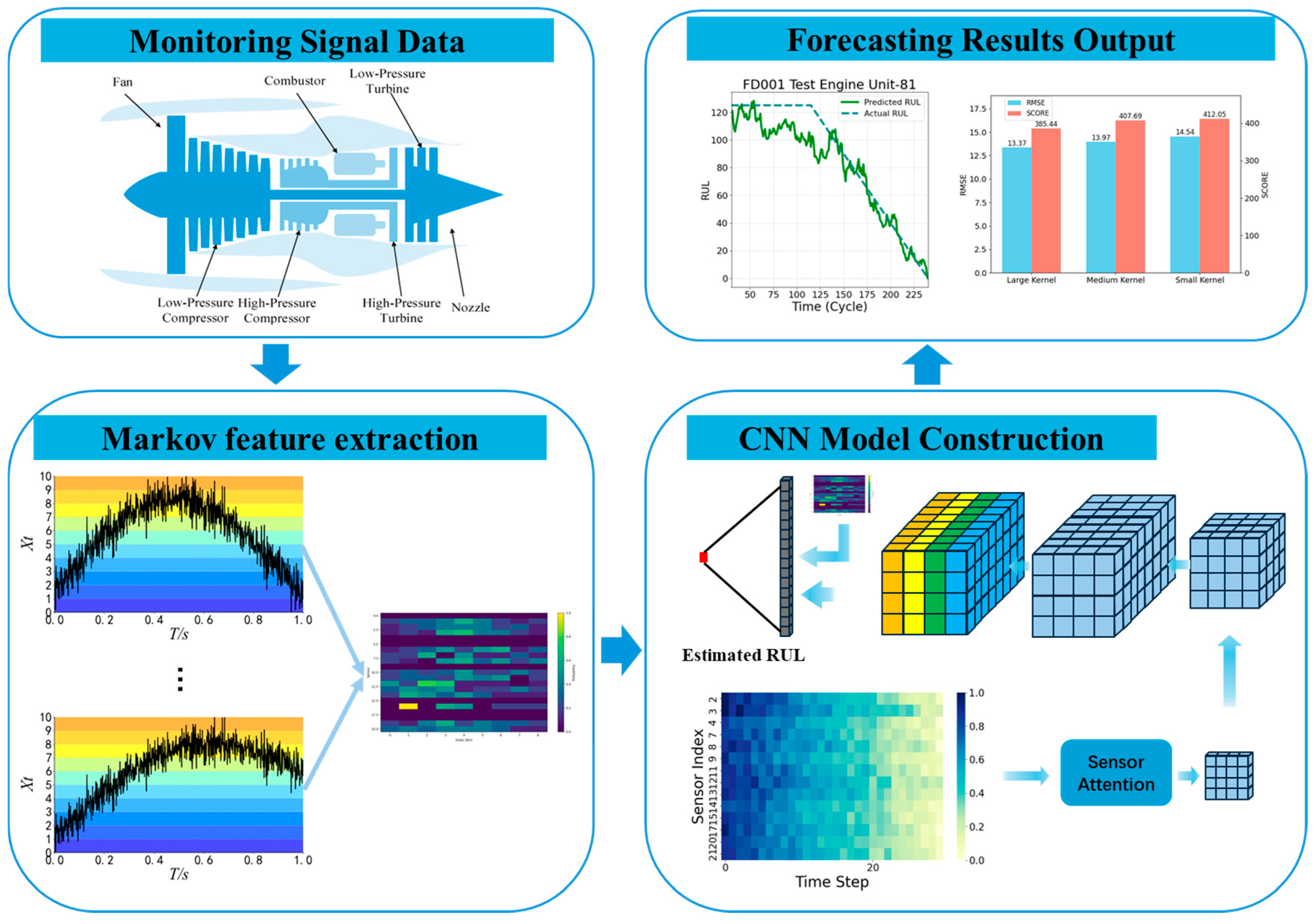
The proposed framework for remaining useful life (RUL) prediction integrates convolutional feature extraction, channel attention, and Markov feature fusion into an end-to-end model for multi-sensor degradation data. The input monitoring signals, represented as a tensor $x\in {\mathbb{R}}^{B\times 1\times W\times S}$, are first processed by convolutional layers with large kernels to extract deterministic temporal–spatial features, capturing both local and mid-range dependencies in degradation trends.

A channel attention mechanism is then applied to enhance the most informative sensor channels. Global average pooling generates compact channel descriptors, which are passed through fully connected layers with non-linear activation and sigmoid normalization to produce adaptive attention weights. These weights refine the convolutional features by emphasizing key channels and suppressing redundant information.

In parallel, a Markov feature extraction module models the stochastic transition characteristics of the degradation process. Specifically, the continuous sensor measurements are first discretized into $N$ states using uniform binning. The transition matrix is then constructed by counting the observed transitions between consecutive states and normalizing each row so that the probabilities sum to one. The resulting transition probabilities are concatenated with the deterministic CNN features to form a hybrid representation, which is processed by fully connected layers with dropout regularization to output the final RUL estimation. This integrated framework jointly captures deterministic degradation dynamics and probabilistic transitions, thereby improving both prediction accuracy and generalization performance. Figure 1 presents the overall workflow of the proposed method.

3. Experimental Setup

3.1. Dataset Description

In this study, the proposed approach is validated using the C-MAPSS [24] (Commercial Modular Aero-Propulsion System Simulation) dataset provided by NASA, which is a well-established benchmark for turbofan engine degradation prediction. The dataset was generated through a high-fidelity simulation model that emulates realistic engine wear and fault progression under various operating conditions.

The complete dataset consists of four subsets (FD001–FD004), each containing multivariate time-series data collected from 21 sensors. Every subset includes a training set and a testing set, corresponding to different combinations of operational settings and fault modes. During the simulation, each engine unit begins from a healthy state but with varying levels of initial wear caused by manufacturing differences. As operation cycles increase, sensor readings gradually reflect degradation until a failure occurs—the final recorded cycle is regarded as the end of the engine’s useful life.

In the training set, the engines are run to failure, and each time step is labeled with its corresponding Remaining Useful Life (RUL) value, which is computed using a piecewise linear degradation model. In the testing set, sensor data for each engine are truncated before failure, and the task is to estimate the RUL for these partially degraded engines. The true RUL values of test units are also provided for model evaluation.

A summary of the dataset configuration is presented in

Table 1. Information of C-MAPSS dataset.

Dataset	Training Units	Testing Units	Operating Conditions	Fault Modes	Training Samples	Testing Samples
FD001	100	100	1	1	17,731	100
FD002	260	259	6	1	48,819	259
FD003	100	100	1	2	21,820	100
FD004	249	248	6	2	57,522	248

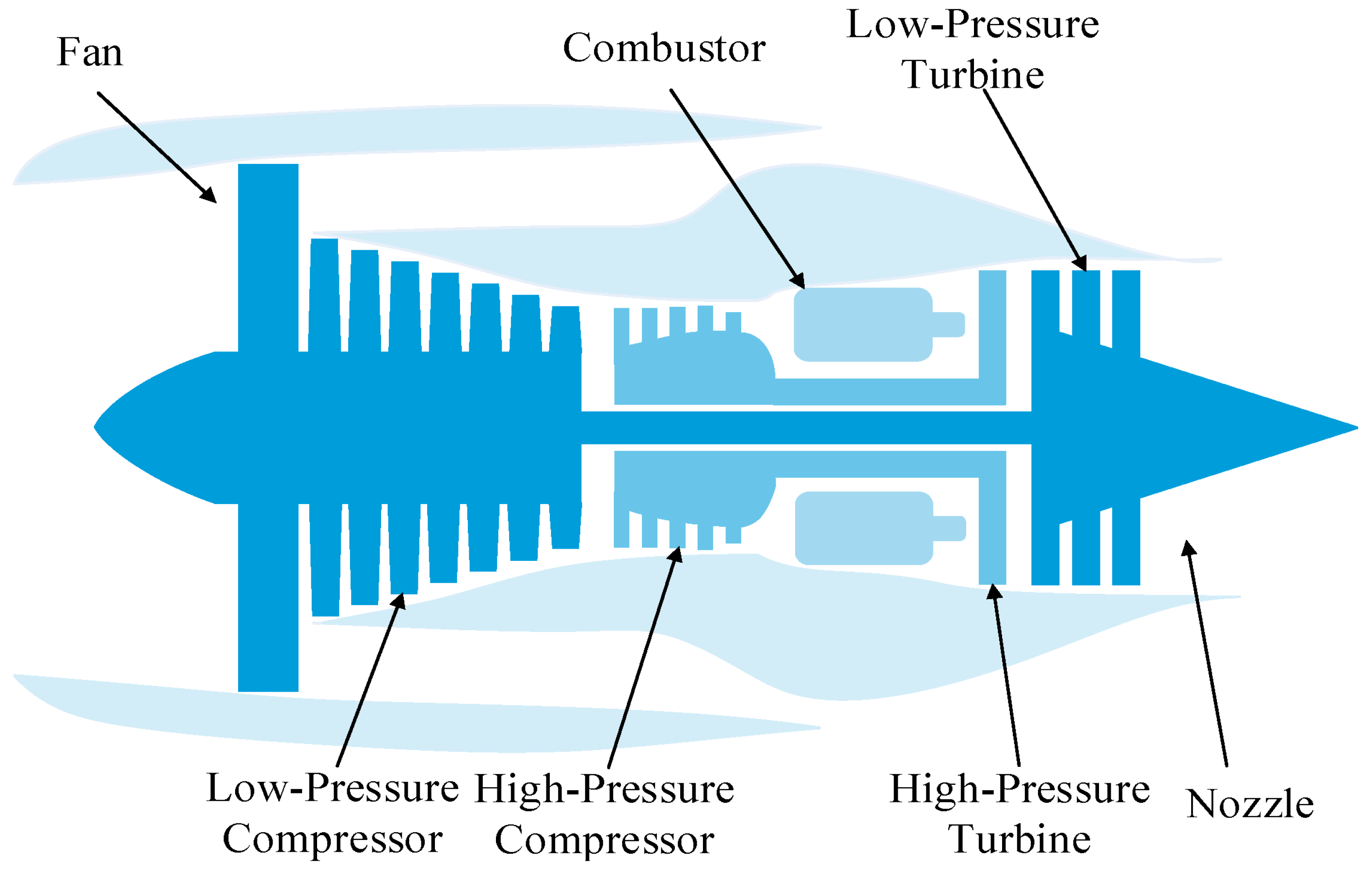
, where FD001 and FD003 involve single operational conditions, while FD002 and FD004 contain multiple operating conditions and higher complexity. All engine measurements are utilized as training samples in this study, and the last recorded cycle of each test engine is adopted for testing. Figure 2 illustrates the simplified schematic of the aircraft engine model used in this study.

3.2. Data Preprocessing

In practical application, degradation of a system tends to be negligible in the initial stage and increases as it approaches run-to-failure. Hence, we utilize a piece-wise linear degradation model to obtain RUL labels with respect to each sample, whose maximum RUL is set as 130 according to the research of Zheng et al. [26]. This fixed maximum RUL represents the initial, nearly undegraded state of the engines, reflecting the upper bound of their remaining useful life before significant degradation occurs, and ensures consistency with established benchmarks for model training and evaluation.

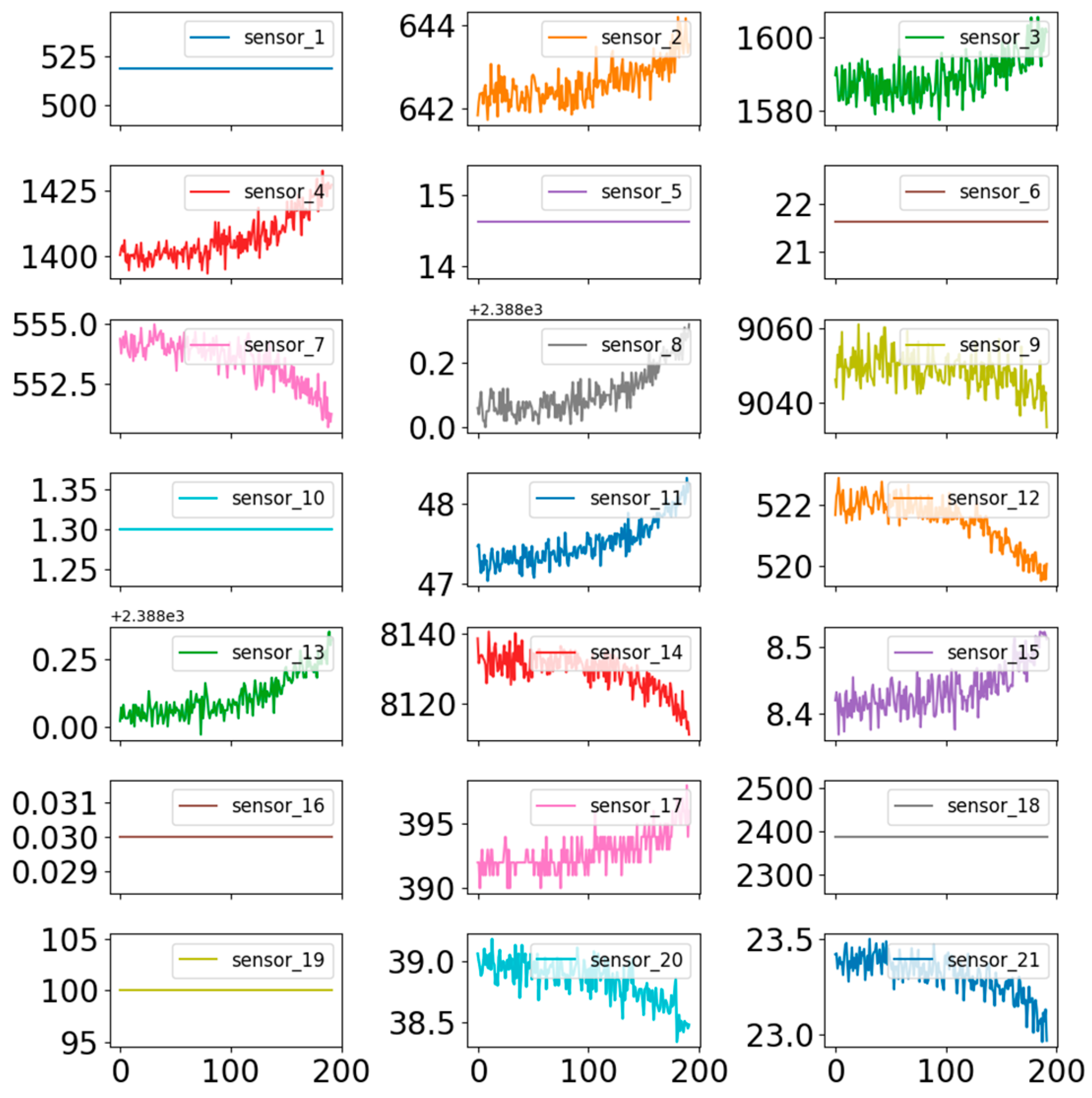
The C-MAPSS dataset provides multivariate temporal measurements from 21 onboard sensors for each turbofan engine. Figure 3 shows the original time-series sensor data of turbofan engine #1 in FD001.Following prior studies, 14 informative sensors were selected as input variables, corresponding to indices [2, 3, 4, 7, 8, 9, 11, 12, 13, 14, 15, 17, 20, and 21]. These sensors effectively capture the degradation trends of the engines and are widely used in performance prediction research [27,28].

To ensure comparability among sensor readings with different scales, all selected measurements are normalized using the min–max normalization technique, transforming each feature to the range [−1, 1]. The normalization process is formulated as:

$$x_{i,j}^{norm}=2\times {\displaystyle \frac{x_{i,j}-x_j^{min}}{x_j^{max}-x_j^{min}}}-1,\forall i\in [1,N], j\in [1,M]$$

(12)

where ${\mathit{x}}_{\mathit{i},\mathit{j}}$ represents the original reading of the $\mathit{j}$-th sensor at the $\mathit{i}$-th time step, and ${\mathit{x}}_{\mathit{i},\mathit{j}}^{\mathit{n}\mathit{o}\mathit{r}\mathit{m}}$ denotes the normalized value. ${\mathit{x}}_{\mathit{j}}^{\mathit{m}\mathit{a}\mathit{x}}$ and ${\mathit{x}}_{\mathit{j}}^{\mathit{m}\mathit{i}\mathit{n}}$ are the maximum and minimum readings of the $\mathit{j}$-th sensor across the entire dataset.

This normalization ensures that all sensor signals contribute equally during model training and prevents features with large numerical ranges from dominating the learning process.

In Remaining Useful Life (RUL) estimation tasks based on multivariate time series, temporal dependencies often contain richer degradation information than isolated data points captured at a single time step. To effectively exploit this temporal correlation, a sliding time window mechanism is employed for data preparation. Specifically, for each engine, sensor readings from consecutive time steps are collected using a fixed-length window of size $N_{tw}$, which advances one time step at a time (i.e., stride = 1), resulting in maximal overlap between consecutive windows. This overlapping design ensures that both short-term and long-term degradation patterns are effectively captured. Segmentation is performed separately for each engine, maintaining a balanced representation of degradation trends across the dataset. The aggregated data within each window are then concatenated to form a high-dimensional feature vector, which serves as input to the proposed network model, enabling consistent and comparable learning across all engines.

3.3. Evaluation Metrics

To quantitatively evaluate the performance of the proposed model in predicting the Remaining Useful Life (RUL) of engine units, two commonly used metrics are adopted: Root Mean Square Error (RMSE) and the prognostic Score $S$ [29]. RMSE measures the average magnitude of prediction errors, reflecting how closely the predicted RUL values (${\mathrm{RUL}}_i^{\mathrm{pred}}$) align with the true RUL (${\mathrm{RUL}}_i$) across all $n$ testing samples, and is defined as

$$RMSE=\sqrt{{\displaystyle \frac{1}{n}}\sum _{i=1}^n{({\mathrm{RUL}}_i^{pred}-{\mathrm{RUL}}_i)}^2}.$$

(13)

A lower RMSE indicates that the predicted values are, on average, closer to the ground truth, which indicates higher prediction accuracy. In practical prognostics, overestimating and underestimating the remaining life have asymmetric consequences: overestimation may lead to unexpected failures, while underestimation could result in unnecessary maintenance. To reflect this asymmetry, the scoring function $S$ is used. The prediction error for the $i$-th sample is defined as

$$d_i={\mathrm{RUL}}_i^{pred}-{\mathrm{RUL}}_i,$$

(14)

and the corresponding individual score is calculated as

$$s_i=\left\{\begin{array}{c}{e}^{{\displaystyle \frac{d_i}{13}}}-1,\mathrm{if}{d}_i<0,\\ e^{{\displaystyle \frac{d_i}{10}}}-1,\mathrm{if}{d}_i\ge 0.\end{array}\right.$$

(15)

The total score is obtained by summing the individual scores of all test samples:

$$S=\sum _{i=1}^n{s}_i.$$

(16)

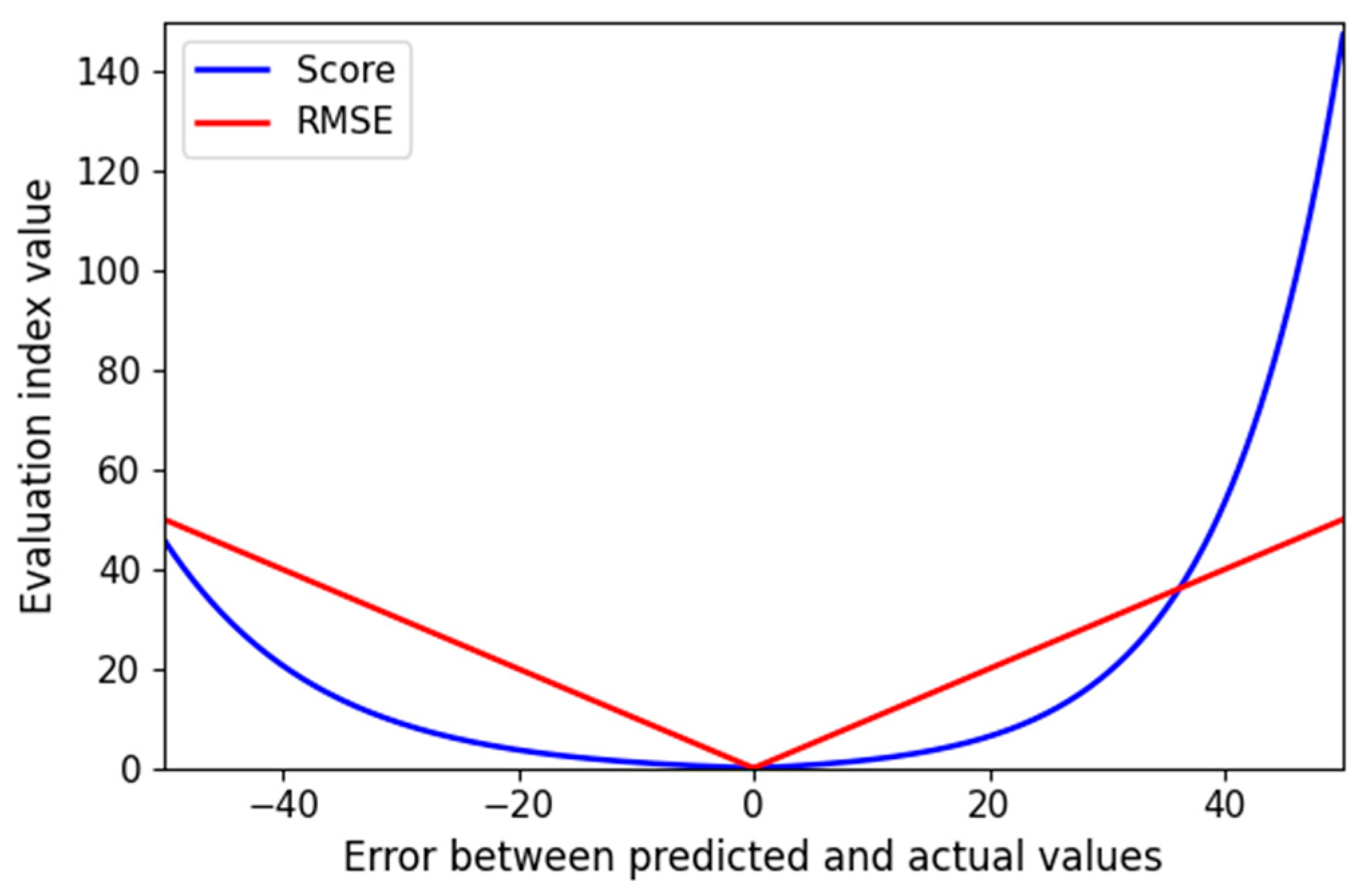
Figure 4 compares two evaluation indicators of the RUL prediction model: the root mean square error (RMSE) and the scoring function. When $d=0$, the predicted RUL equals the actual RUL, and both indicators yield zero. As the error magnitude increases, their values rise correspondingly. The RMSE provides a symmetric measure of the overall prediction deviation, assigning equal penalties to early and late predictions. In contrast, the scoring function adopts an asymmetric design: early predictions ($d<0$) incur relatively mild penalties, whereas late predictions ($d>0$) are penalized more heavily. This design reflects the practical consideration that early maintenance is generally preferable to delayed maintenance in industrial applications.

3.4. Hyperparameter and Training Details

Each input to the model is a 2D tensor of shape (N_tw, N_channels), where N_tw = 30 is the sliding window length (time steps) and N_channels = 14 corresponds to the selected sensor channels [2, 3, 4, 7, 8, 9, 11, 12, 13, 14, 15, 17, 20, 21]. For training, multiple sliding windows are extracted from all engines, forming a dataset of size N_samples. The sensor readings in each window are normalized per channel using z-score normalization to ensure that temporal patterns of all sensors are on a comparable scale for effective learning by the convolutional layers.

Key hyperparameters and training settings for the proposed RUL prediction model are summarized in

Table 2. Summary of Hyperparameters for the Proposed RUL Prediction Model.

Hyperparameter/Setting	Value/Description
Convolution kernel sizes.	[15 × 1, 11 × 1, 7 × 1, 3 × 1]
Sliding window size (N_tw)	30
Stride/Overlap	1
Learning rate	1 × 10−4
Batch size	128
Epochs	200
Dropout probability	0.3
Optimizer	Adam
Markov feature bin count	10

. During training, a sliding window of length 30 with stride 1 was used to capture temporal dependencies in the multivariate sensor sequences. The model was optimized using Adam with a learning rate of 1 × 10⁻⁴, trained for 200 epochs with a batch size of 128. Dropout with a probability of 0.3, together with weight decay, was applied to reduce overfitting. A fixed train–validation split was adopted, where a fixed engine-level split was used for validation; no cross-validation or early stopping was used to maintain consistent benchmarking across experiments. The Markov feature representation was quantized into 10 bins to model probabilistic degradation transitions, which enables capturing discrete degradation states for RUL prediction.

The window length of 30 time steps was selected to provide sufficient temporal span for capturing medium-term degradation dynamics while avoiding excessive smoothing of short-term variations. This ensures that the model receives enough historical context to learn meaningful degradation patterns without introducing unnecessary computational overhead or diluting recent sensor information.

4. Results and Discussion

This section assesses the performance of the proposed remaining useful life (RUL) prediction model. The evaluation considers the influence of key parameters, including convolutional kernel size and time window length, and benchmarks the model against mainstream neural network architectures to validate its effectiveness. Comparative experiments on the C-MAPSS dataset further highlight the superiority of the proposed approach. To reduce the impact of randomness, all reported results represent the average of 10 independent trials. All experiments were conducted on a system equipped with an Intel Core i5-12400 CPU and an NVIDIA GeForce RTX 4060 Ti GPU.

4.1. Quantitative Results on C-MAPSS

Table 3. Performance comparison of different methods on C-MAPSS dataset.

Method	FD001		FD002		FD003		FD004
	RMSE	Score	RMSE	Score	RMSE	Score	RMSE	Score
NN [27]	14.8	496.3	25.64	18,255	15.22	522.3	25.8	20,422
DNN [27]	13.56	348.3	24.61	15,622	13.93	364.3	24.31	16,223
RNN [27]	13.44	339.2	24.03	14,245	13.36	315.7	24.02	13,931
LSTM [27]	13.52	431.7	24.42	14,459	13.54	347.3	24.21	14,322
MODBNE [30]	15.04	334.23	25.05	5585.34	12.51	421.91	28.66	6557.62
DBN [30]	15.21	417.59	27.12	9031.64	14.71	442.43	29.88	7954.51
CNN-LSTM-Attention [31]	15.97	-	14.45	-	13.9	-	16.63	-
Our method	12.62	366.98	13.33	6607.44	11.35	391.85	13	3805.35

presents a comprehensive performance comparison of various methods on the four C-MAPSS subsets in terms of RMSE and the corresponding Score metric. Among the baseline methods, traditional neural networks (NN), deep neural networks (DNN), recurrent neural networks (RNN), and LSTM achieve moderate predictive accuracy. For instance, NN achieves RMSE values of 14.80, 25.64, 15.22, and 25.80 on FD001–FD004, respectively, while LSTM achieves slightly better results of 13.52, 24.42, 13.54, and 24.21. Overall, RMSE values for these models range from 13.36 to 25.80 across the datasets, reflecting that standard neural network architectures can capture degradation trends to a certain extent but still suffer from reduced performance under complex scenarios such as FD002 and FD004.

Probabilistic models, including MODBNE and DBN, exhibit more variable results. MODBNE achieves the lowest RMSE of 12.51 on FD003 but performs poorly on FD004, with an RMSE of 28.66. Similarly, DBN demonstrates higher RMSE values of 27.12 and 29.88 on FD002 and FD004, respectively, indicating inconsistent predictive capability across datasets. This suggests that while probabilistic methods can model uncertainty, they may not generalize well under diverse operating conditions.

Deep hybrid models combining convolutional and recurrent architectures, such as CNN-LSTM-Attention [31], show improved RMSE compared with standard neural networks, achieving 15.97, 14.45, 13.90, and 16.63 on FD001–FD004. Although these models integrate sequence modeling and attention mechanisms, their performance is still outperformed by the proposed method, particularly on complex subsets like FD002 and FD004.

In contrast, our proposed method consistently achieves the lowest RMSE values of 12.62, 13.33, 11.35, and 13.00 on FD001–FD004, representing significant improvements over all baseline methods. For example, compared with the next best-performing model, RNN, our method reduces RMSE by 0.82, 10.69, 2.01, and 11.02 for FD001–FD004. Corresponding Score metrics further confirm the reliability of our predictions. Our method attains scores of 366.98, 6607.44, 391.85, and 3805.35 on FD001–FD004, showing more balanced performance compared with baseline models that often exhibit extreme fluctuations, such as DBN, which reaches 9031.64 and 7954.51 on FD002 and FD004.

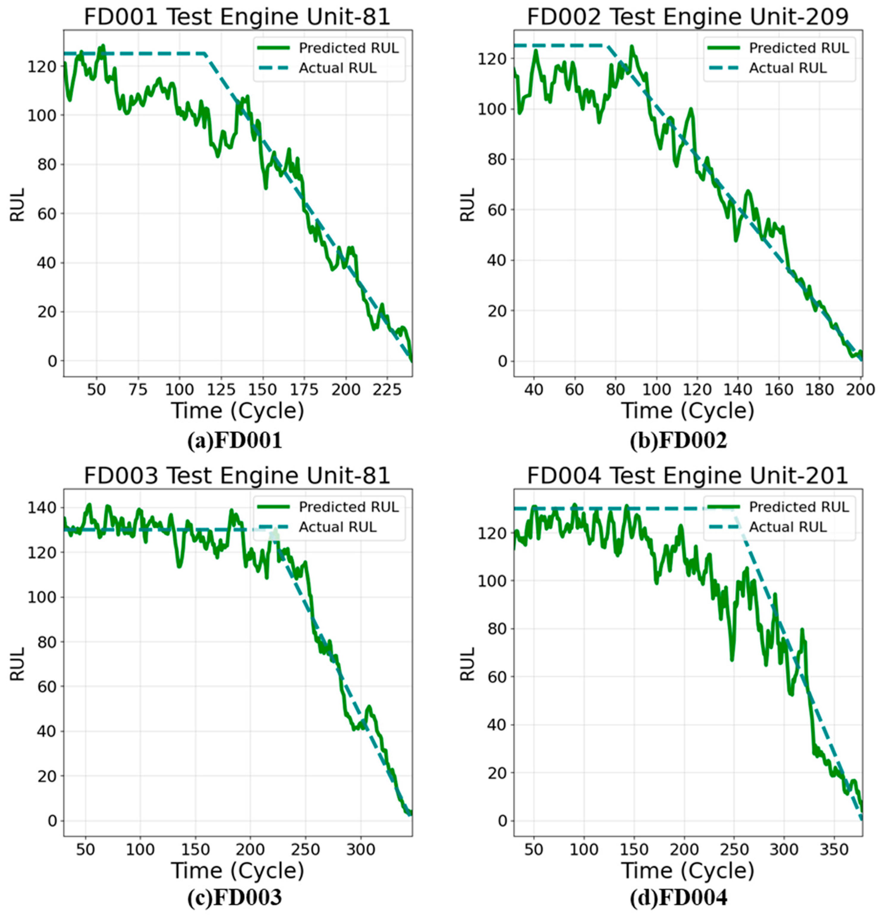
These results demonstrate that the proposed approach not only improves predictive accuracy but also maintains stable performance across both simple and complex datasets. Figure 5 illustrates representative RUL prediction samples for the four subsets, highlighting the method’s robustness in capturing diverse degradation patterns.

4.2. Ablation Study

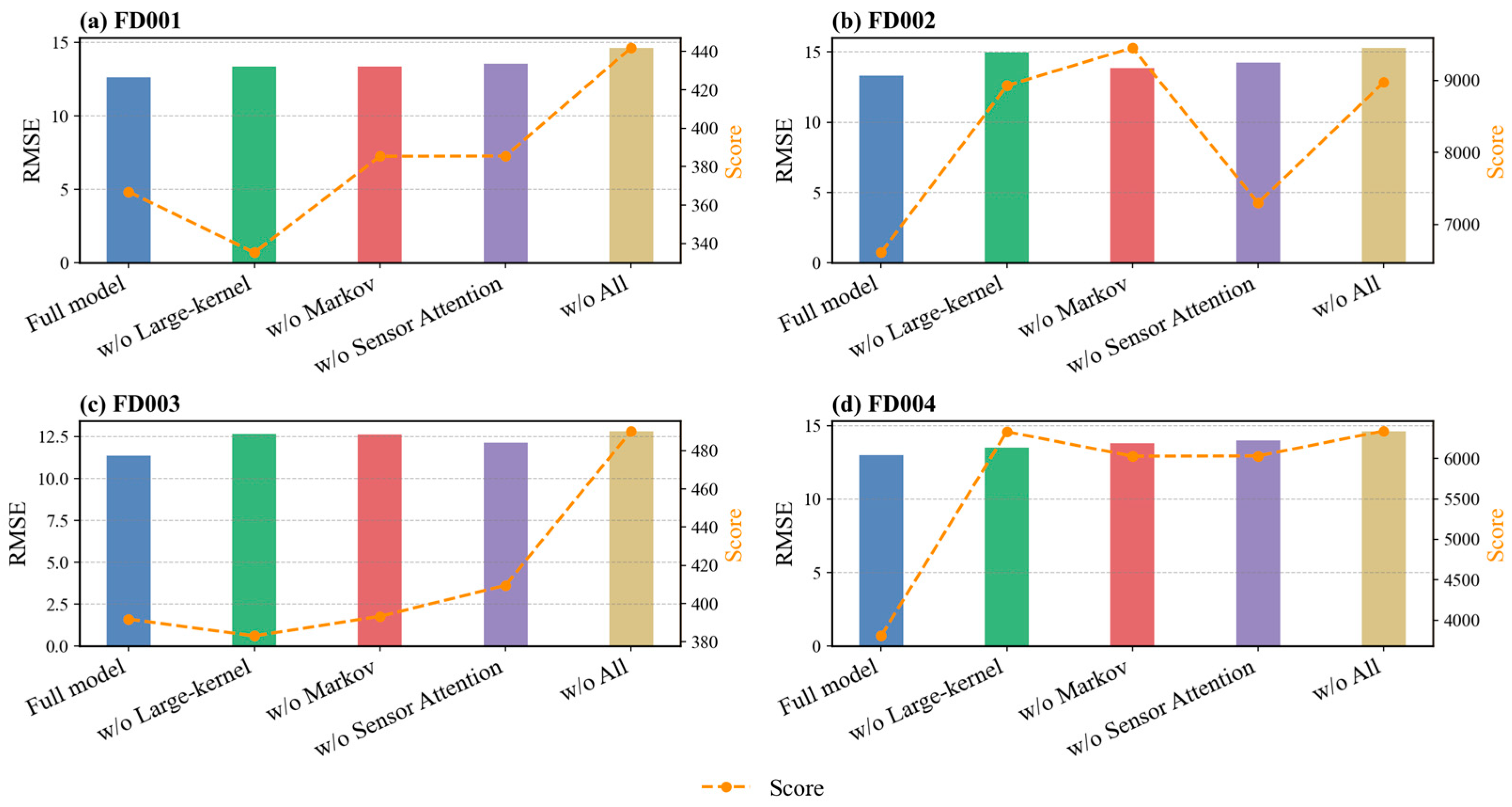
An ablation study was conducted to evaluate the contributions of large-kernel convolution, Markov features, and sensor attention.

Table 4. Ablation study on the effects of large-kernel convolution and Markov features.

Method	FD001		FD002		FD003		FD004
	RMSE	Score	RMSE	Score	RMSE	Score	RMSE	Score
Full model (ours)	12.62	366.98	13.33	6607.44	11.35	391.85	13	3805.35
(w/o) Large-kernel	13.38	335.32	14.99	8928.24	12.67	383.1	13.51	6331.85
(w/o) Markov features	13.37	385.44	13.87	9456.79	12.64	393.32	13.81	6029.09
(w/o) Sensor Attention	13.57	385.58	14.23	7296.39	12.15	409.53	14	6032.08
(w/o) All	14.61	441.93	15.27	8977.49	12.81	490.29	14.6	6341.55

Bold values indicate the best performance among the compared methods.

summarizes the RMSE and Score metrics for the full model and four ablation variants across the four datasets (FD001–FD004). Removing the large-kernel convolution increases the RMSE relative to the full model by 0.76, 1.66, 1.32, and 0.51 for FD001, FD002, FD003, and FD004, respectively. Excluding the Markov features results in increases of 0.75, 0.54, 1.29, and 0.81, whereas removing the sensor attention causes increases of 0.95, 0.90, 0.80, and 1.00, respectively. When all three components are removed (w/o All), the RMSE further rises to 14.61, 15.27, 12.81, and 14.60 for FD001–FD004, highlighting the combined importance of these components. These results demonstrate that large-kernel convolution enhances feature extraction by capturing long-range dependencies, Markov features model temporal degradation patterns, and sensor attention emphasizes informative channels; together, they produce the lowest prediction errors.

The effects on the Score metric are presented in Table 4 and Figure 6. Removing the large-kernel convolution leads to Score changes of −31.66, 2320.80, −8.75, and 2526.50 for FD001–FD004. Excluding the Markov features results in changes of 18.46, 2849.35, 1.47, and 2223.74, while removing the sensor attention results in Score increases of 18.60, 688.95, 17.68, and 2226.73, respectively. When all three components are removed, the Scores increase to 441.93, 8977.49, 490.29, and 6341.55, indicating less stable and less reliable RUL predictions. Overall, the full model achieves both lower RMSE and more balanced Scores across all datasets, demonstrating that the combination of large-kernel convolution, Markov features, and sensor attention significantly improves RUL prediction accuracy.

4.3. Sensor-Level Attention Analysis

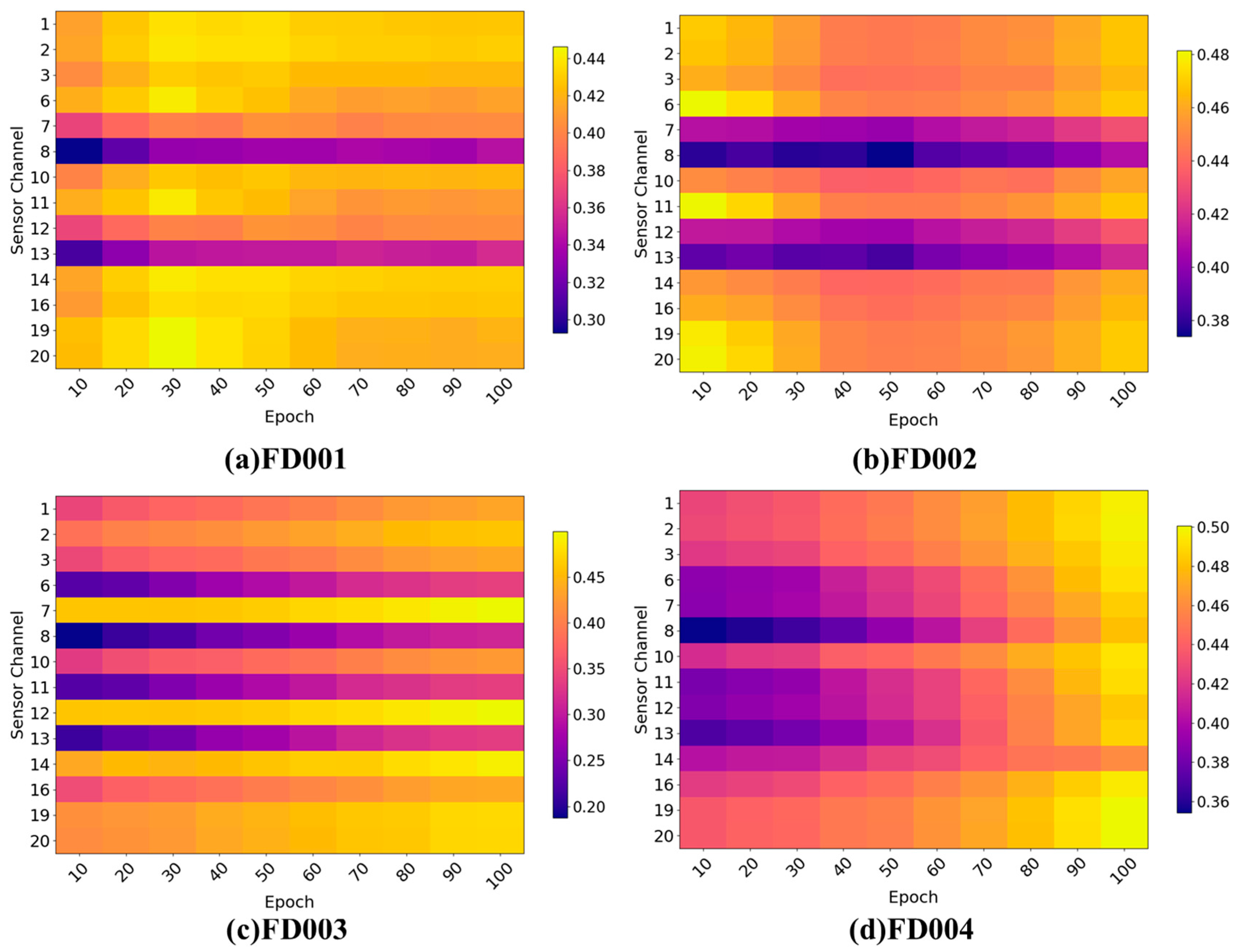
Figure 7 illustrates the evolution of sensor-level attention weights across the four datasets (FD001–FD004), providing insights into how the attention mechanism differentiates sensor importance during training. The results demonstrate that the proposed attention module not only enhances feature representation but also functions as an implicit sensor selection mechanism.

For FD001, the attention distributions show highly consistent patterns: Sensors 1, 5, 10, 16, and 18 receive persistently high attention across all epochs, indicating that they carry the most informative degradation-related signals for RUL estimation. Conversely, Sensors such as 6 and 9 remain at low attention levels throughout training, suggesting limited contribution or redundancy in this operating condition.

In FD002, Sensors 1, 2, 3, 5, and 18 exhibit progressively increasing attention weights. This gradual strengthening of importance reflects the model’s adaptation to the mixed operating conditions in FD002 and highlights its ability to emphasize dataset-specific informative channels while down-weighting less relevant ones.

For FD003 and FD004, although the overall attention distribution appears more uniform due to the more complex multi-operating-condition settings, certain sensors still dominate the learned patterns. Low-importance channels are consistently suppressed, demonstrating that the model integrates complementary information from multiple sensors while mitigating the influence of noise or weakly correlated signals.

Overall, the attention mechanism effectively identifies and prioritizes informative channels across all datasets. Sensors with persistently low attention are implicitly filtered out, reducing irrelevant or noisy inputs and enhancing both the robustness and interpretability of the RUL prediction model. The lighter color intensities in the bar plots visually highlight sensors with higher attention weights, providing a clear indication of their relative contributions.

4.4. Effects of Convolution Kernel Size and Time Window

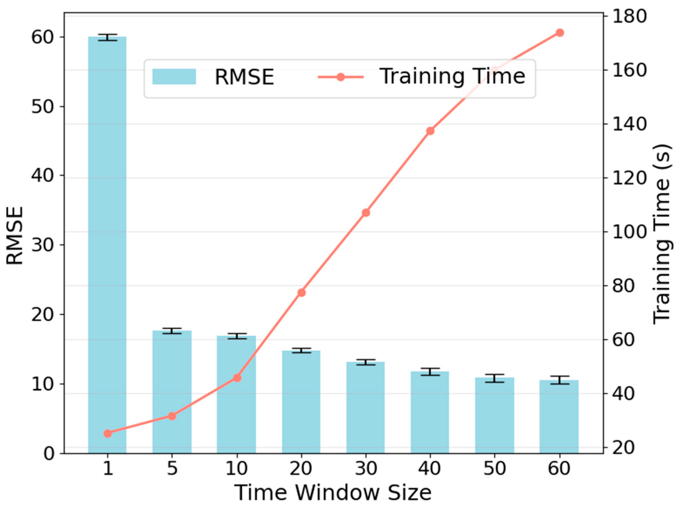
The effect of the time window size in sample preparation on the network performance is further analyzed, as shown in Figure 8. Larger time windows generally lead to lower RMSE values, indicating that a longer temporal context allows the network to capture more comprehensive information from the sensor signals. Specifically, a notable reduction in RMSE is observed when the time window increases from 20 to 30, suggesting that including sufficient past cycles is crucial for accurate RUL estimation. Beyond a window size of 30, the improvement in prediction accuracy becomes marginal, implying a diminishing return for excessively large windows. At the same time, the computational cost of training grows with the time window size. Longer windows require processing more input data per sample, resulting in increased training time. Considering both predictive accuracy and computational efficiency, a time window of 30 is selected as the default for the sub-dataset FD001.

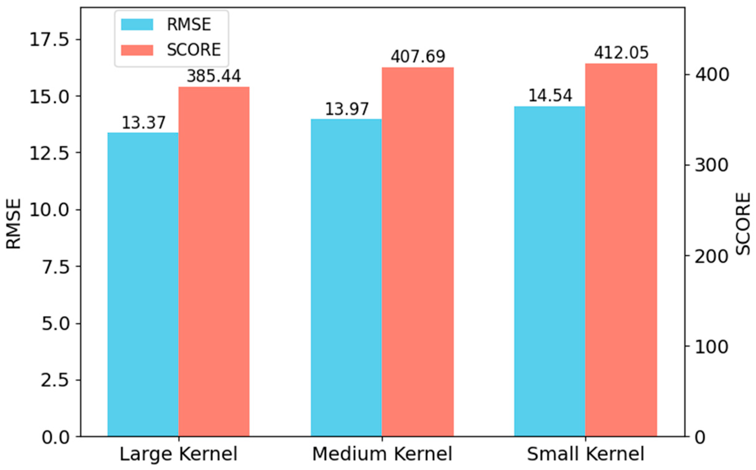
Models with larger convolution kernels demonstrate superior predictive accuracy, as evidenced by lower RMSE and SCORE values in Figure 9. The four-layer configuration with kernel sizes (15, 1)–(11, 1)–(7, 1)–(3, 1) achieves the best performance (RMSE = 13.37, SCORE = 385.44), indicating its stronger capability to capture long-range temporal dependencies in sensor sequences. In contrast, the medium configuration (9, 1)–(7, 1)–(5, 1)–(3, 1) yields slightly inferior results (RMSE = 13.97, SCORE = 407.69), while the smallest kernel setup (5, 1)–(3, 1)–(3, 1)–(3, 1) performs the worst (RMSE = 14.54, SCORE = 412.05). These results highlight that larger receptive fields enhance the network’s ability to extract degradation features essential for accurate RUL prediction. These findings demonstrate that adopting larger kernels in shallow layers and smaller ones in deeper layers improves hierarchical temporal feature representation, thus enhancing RUL prediction accuracy.

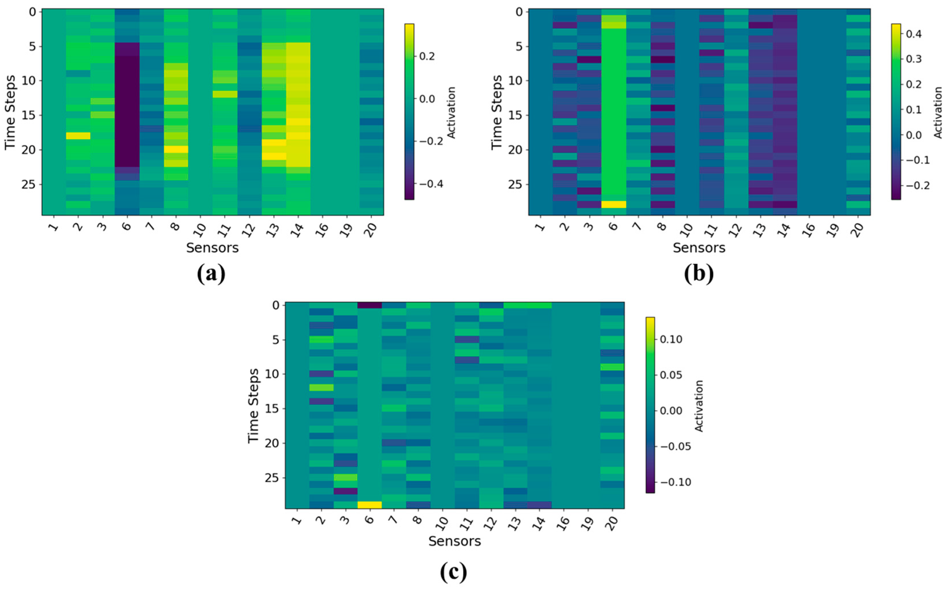
Figure 10 compares the activation maps generated by large-, medium-, and small-kernel convolutions, revealing that kernel size has a substantial impact on temporal–sensor feature extraction. The large-kernel convolution produces smoother and more continuous activation patterns across time, indicating its superior ability to capture long-range temporal dependencies that characterize gradual degradation processes. It also exhibits stronger sensor-level discrimination, as shown by the stable high-activation bands on key sensors such as Sensor 5, whereas medium- and small-kernel designs yield more fragmented and inconsistent responses. Moreover, the large kernel demonstrates enhanced robustness to noise, with noticeably fewer random local activations and a cleaner background, reflecting its improved temporal–spatial aggregation capability. Finally, the large-kernel convolution generates higher and more stable activation magnitudes in degradation-relevant regions, suggesting more salient and reliable feature extraction. Collectively, these results confirm that large-kernel convolutions provide more informative, robust, and discriminative representations for multivariate sensor sequences, leading to improved health modeling performance.

In this study, we compared the computational cost and inference efficiency of three convolutional kernel designs: small, medium, and large. The small-kernel model has the fewest parameters (0.130 M) and lowest FLOPs (12.851 M), with an average inference time of 4.395 ms per batch, making it the fastest among the three. The medium-kernel model slightly increases the parameter count (0.135 M) and FLOPs (16.117 M), resulting in an average inference time of 4.479 ms per batch. The large-kernel model has the largest parameter size (0.164 M) and highest FLOPs (34.261 M), with an average inference time of 4.897 ms per batch. Overall, model complexity is positively correlated with inference time. The small- and medium-kernel models achieve low computational cost while maintaining almost identical inference speed, whereas the large-kernel model, despite higher computation, incurs only a modest increase in latency. Additionally, all models show noticeably longer inference time during the first epoch, likely due to GPU initialization overhead. The detailed experimental results are summarized in

Table 5. Computational Cost and Average Inference Time of Different Kernel Designs.

Model	Params (M)	MACs (M)	Average Inference Time (ms/Batch = 128)
Small-kernel	0.130	12.851	4.395
Mid-kernel	0.135	16.117	4.479
Large-kernel	0.164	34.261	4.897

.

5. Conclusions

Despite the superior performance, the proposed method has certain limitations. The integration of large-kernel convolutions, attention mechanisms, and Markov feature fusion increases computational cost, which may affect training efficiency and deployment on resource-constrained devices. Additionally, the discretization of continuous degradation states in Markov feature extraction can influence model sensitivity and prediction stability, as poorly chosen state boundaries may lead to information loss or uneven state occupancy. The method has been evaluated primarily on the C-MAPSS dataset, which may limit its generalization to real industrial scenarios.

Moreover, the proposed method may have limitations under extreme or highly non-stationary operating conditions. Specifically, rapid transition regimes could reduce the responsiveness of large-kernel convolutions, potentially underrepresenting short-term degradation patterns. In addition, Markov features may become less reliable when engines exhibit irregular or non-monotonic degradation behaviors, which could affect transition probabilities and prediction stability. Sensor attention might also be biased under noise bursts or partial sensor dropout, possibly causing the model to overemphasize corrupted channels and produce less stable predictions.

Nevertheless, the combination of deterministic convolutional features, stochastic Markov transitions, and channel attention enables the network to capture both local degradation patterns and probabilistic state evolution while reducing the influence of irrelevant or noisy sensor channels. Extensive experiments on benchmark datasets demonstrate that the proposed approach outperforms conventional CNN-based prognostic models, achieving lower RMSE and more balanced predictive results.

The main contributions and findings of this work can be summarized as follows:

• Comprehensive feature representation: The network combines deterministic convolutional features with stochastic Markov transition features, capturing both local degradation patterns and probabilistic state evolution.
• Enhanced temporal–spatial modeling: Large-kernel convolution layers extract rich temporal–spatial features from multi-sensor time-series data.
• Adaptive feature emphasis: The channel attention mechanism selectively emphasizes the most informative sensor channels, improving sensitivity to degradation-relevant signals.

For future work, several directions are envisaged: validating the approach on real-world industrial datasets with diverse operating conditions, integrating additional contextual information such as operational and environmental variables, exploring lightweight model architectures suitable for edge deployment, and extending the framework to handle multi-component systems. Furthermore, combining the proposed approach with physics-informed modeling or uncertainty quantification could enhance interpretability, provide confidence bounds, and improve prediction reliability, supporting more effective condition-based maintenance strategies.

References

- Seid Ahmed, Y.; Abubakar, A.A.; Arif, A.F.M.; Al-Badour, F.A. Advances in Fault Detection Techniques for Automated Manufacturing Systems in Industry 4.0. Front. Mech. Eng. 2025, 11, 1564846. [Google Scholar] [CrossRef]
- Neupane, D.; Bouadjenek, M.R.; Dazeley, R.; Aryal, S. Data-Driven Machinery Fault Diagnosis: A Comprehensive Review. Neurocomputing 2025, 627, 129588. [Google Scholar] [CrossRef]
- Xiao, B.; Zhong, J.; Bao, X.; Chen, L.; Bao, J.; Zheng, Y. Digital Twin-Driven Prognostics and Health Management for Industrial Assets. Sci. Rep. 2024, 14, 13443. [Google Scholar] [CrossRef] [PubMed]
- Ciang, C.C.; Lee, J.-R.; Bang, H.-J. Structural Health Monitoring for a Wind Turbine System: A Review of Damage Detection Methods. Meas. Sci. Technol. 2008, 19, 122001. [Google Scholar] [CrossRef]
- Luo, Y.; Zhu, M.; Chen, T.; Zheng, Z. Remaining Useful Life Prediction for Stratospheric Airships Based on a Channel and Temporal Attention Network. Commun. Nonlinear Sci. Numer. Simul. 2025, 143, 108634. [Google Scholar] [CrossRef]
- Tsallis, C.; Papageorgas, P.; Piromalis, D.; Munteanu, R.A. Application-Wise Review of Machine Learning-Based Predictive Maintenance: Trends, Challenges, and Future Directions. Appl. Sci. 2025, 15, 4898. [Google Scholar] [CrossRef]
- Wahid, A.; Breslin, J.G.; Intizar, M.A. TCRSCANet: Harnessing Temporal Convolutions and Recurrent Skip Component for Enhanced RUL Estimation in Mechanical Systems. Hum.-Centric Intell. Syst. 2024, 4, 1–24. [Google Scholar] [CrossRef]
- Wang, H.; Wu, S.; Yu, F.; Bi, Y.; Xu, Z. Study on Remaining Useful Life Prediction of Sliding Bearings in Nuclear Power Plant Shielded Pumps Based on Nearest Similar Distance Particle Filtering. Ann. Nucl. Energy 2024, 223, 111625. [Google Scholar] [CrossRef]
- Wan, S.; Li, X.; Zhang, Y.; Liu, S.; Hong, J.; Wang, D. Bearing Remaining Useful Life Prediction with Convolutional Long Short-Term Memory Fusion Networks. Reliab. Eng. Syst. Saf. 2022, 224, 108528. [Google Scholar] [CrossRef]
- Malashin, I.; Tynchenko, V.; Gantimurov, A.; Nelyub, V.; Borodulin, A. Applications of Long Short-Term Memory (LSTM) Networks in Polymeric Sciences: A Review. Polymers 2024, 16, 2607. [Google Scholar] [CrossRef]
- Zhang, Y.; Xiong, R.; He, H.; Pecht, M.G. Long Short-Term Memory Recurrent Neural Network for Remaining Useful Life Prediction of Lithium-Ion Batteries. IEEE Trans. Veh. Technol. 2018, 67, 5695–5705. [Google Scholar] [CrossRef]
- Hou, G.; Xu, S.; Zhou, N.; Yang, L.; Fu, Q. Remaining Useful Life Estimation Using Deep Convolutional Generative Adversarial Networks Based on an Autoencoder Scheme. Comput. Intell. Neurosci. 2020, 2020, 9601389. [Google Scholar] [CrossRef]
- Yang, L.; Jiang, Y.; Zeng, K.; Peng, T. Rolling Bearing Remaining Useful Life Prediction Based on CNN-VAE-MBiLSTM. Sensors 2024, 24, 2992. [Google Scholar] [CrossRef]
- Shakir, M.; Kumaran, U.; Rakesh, N. Enhanced Temporal Attention-Based LSTM Model for Air Quality Forecasting. Int. J. Inf. Technol. 2025, 1–9. [Google Scholar] [CrossRef]
- Tran, K.; Vu, H.-C.; Pham, L.; Boudaoud, N.; Nguyen, H.-S.-H. Robust-MBDL: A Robust Multi-Branch Deep-Learning-Based Model for Remaining Useful Life Prediction of Rotating Machines. Mathematics 2024, 12, 1569. [Google Scholar] [CrossRef]
- Zhao, Z.; Wu, J.; Wong, D.; Sun, C.; Yan, R. Probabilistic Remaining Useful Life Prediction Based on Deep Convolutional Neural Network. In Proceedings of the 9th International Conference on Through-life Engineering Service, Cranfield, UK, 3–4 November 2020. [Google Scholar] [CrossRef]
- Kiranyaz, S.; Avci, O.; Abdeljaber, O.; Ince, T.; Gabbouj, M.; Inman, D.J. 1D Convolutional Neural Networks and Applications: A Survey. Mech. Syst. Signal Process. 2021, 151, 107398. [Google Scholar] [CrossRef]
- Ding, H.; Hou, H.; Wang, L.; Cui, X.; Yu, W.; Wilson, D.I. Application of Convolutional Neural Networks and Recurrent Neural Networks in Food Safety. Foods 2025, 14, 247. [Google Scholar] [CrossRef]
- Li, X.; Chu, Y.; Wu, X. 3D Convolutional Neural Network Based on Spatial-Spectral Feature Pictures Learning for Decoding Motor Imagery EEG Signal. Front. Neurorobotics 2024, 18, 1485640. [Google Scholar] [CrossRef] [PubMed]
- Yamashita, R.; Nishio, M.; Do, R.K.G.; Togashi, K. Convolutional Neural Networks: An Overview and Application in Radiology. Insights Imaging 2018, 9, 611–629. [Google Scholar] [CrossRef]
- Zhang, Z.; Tang, A.; Zhang, T. A Transfer-Based Convolutional Neural Network Model with Multi-Signal Fusion and Hyperparameter Optimization for Pump Fault Diagnosis. Sensors 2023, 23, 8207. [Google Scholar] [CrossRef]
- He, Y.; Su, H.; Zio, E.; Peng, S.; Fan, L.; Yang, Z.; Yang, Z.; Zhang, J. A Systematic Method of Remaining Useful Life Estimation Based on Physics-Informed Graph Neural Networks with Multisensor Data. Reliab. Eng. Syst. Saf. 2023, 237, 109333. [Google Scholar] [CrossRef]
- Heimes, F.O. Recurrent Neural Networks for Remaining Useful Life Estimation. In Proceedings of the 2008 International Conference on Prognostics and Health Management, Denver, CO, USA, 6–9 October 2008; pp. 1–6. [Google Scholar]
- Saxena, A.; Simon, D.; Eklund, N. Damage Propagation Modeling for Aircraft Engine Prognostics. In Proceedings of the Prognostics and Health Manage, Washington, DC, USA, 11–13 June 2008. [Google Scholar]
- Jiang, W.; Xu, Y.; Shan, Y.; Liu, H. Degradation Tendency Measurement of Aircraft Engines Based on FEEMD Permutation Entropy and Regularized Extreme Learning Machine Using Multi-Sensor Data. Energies 2018, 11, 3301. [Google Scholar] [CrossRef]
- Zheng, S.; Ristovski, K.; Farahat, A.; Gupta, C. Long Short-Term Memory Network for Remaining Useful Life Estimation. In Proceedings of the 2017 IEEE International Conference on Prognostics and Health Management (ICPHM), Piscataway, NJ, USA, 19–21 June 2017; pp. 88–95. [Google Scholar]
- Li, X.; Ding, Q.; Sun, J.-Q. Remaining Useful Life Estimation in Prognostics Using Deep Convolution Neural Networks. Reliab. Eng. Syst. Saf. 2018, 172, 1–11. [Google Scholar] [CrossRef]
- Li, H.; Cao, P.; Wang, X.; Li, Y.; Yi, B.; Huang, M. Pre-Training Enhanced Unsupervised Contrastive Domain Adaptation for Industrial Equipment Remaining Useful Life Prediction. Adv. Eng. Inform. 2024, 60, 102517. [Google Scholar] [CrossRef]
- Zhao, Z.; Liang, B.; Wang, X.; Lu, W. Remaining Useful Life Prediction of Aircraft Engine Based on Degradation Pattern Learning. Reliab. Eng. Syst. Saf. 2017, 164, 74–83. [Google Scholar] [CrossRef]
- Zhang, C.; Lim, P.; Qin, A.K.; Tan, K.C. Multiobjective Deep Belief Networks Ensemble for Remaining Useful Life Estimation in Prognostics. IEEE Trans. Neural Netw. Learn. Syst. 2017, 28, 2306–2318. [Google Scholar] [CrossRef]
- Deng, S.; Zhou, J. Prediction of Remaining Useful Life of Aero-Engines Based on CNN-LSTM-Attention. Int. J. Comput. Intell. Syst. 2024, 17, 232. [Google Scholar] [CrossRef]