Multi-Strategy Sailfish Optimizer: Novel Algorithm with Dynamic Sardine Population and Improved Search Technique for Efficient Robot Path Planning

Abstract

The sailfish optimizer is a recent swarm-intelligence-based optimization algorithm which mimics the hunting behavior of sailfish in the ocean. It consists of two types of populations, namely, sailfish and sardine, where sailfish represent the candidate solutions and sardines freely maneuver in the search space. Existing research studies have shown that the sailfish optimizer suffers from limited global exploration capability, with local optimum stagnation and slow convergence speed. To address these limitations, an improved sailfish optimizer, namely, the Multi-Strategy Sailfish Optimizer, is proposed in this study. This improved version incorporates a modified search strategy for both sailfish and sardines, a non-linear attack power parameter, an improved hunting procedure, and a dynamic sardine population. The impact of all suggested improvements is analyzed experimentally. Several experiments with single-objective problems presented at the Congress on Evolutionary Computation in 2022 are performed to prove the effectiveness and efficiency of the proposed algorithm. This improved algorithm is compared with well-known optimization algorithms, such as the whale optimization algorithm, the sine–cosine algorithm, etc., and improved variants of those algorithms. A convergence behavior analysis is also performed using convergence graphs. Furthermore, the significance of the work is statistically validated. The analysis indicates that the Multi-Strategy Sailfish Optimizer performs significantly better than other optimization algorithms. It is also applied to solve the tension/compression spring design problem and the mobile robot path planning problem.

1. Introduction

Nature-inspired optimization algorithms (NIOAs) are a set of algorithms that are useful for finding optimal/near-optimal solutions to complex problems, such as the traveling salesman problem (TSP) [1], robot path planning [2], natural language processing [3], scheduling problems [4,5], complex engineering problems [6,7,8], optimizing network topology design [9], classification of ECG signals [10], manufacturing processes [11], electrical engineering [12], and control engineering [13], among others. Applications of NIOAs in diversified areas of engineering and the sciences have made them the preferred choice of the research community [14,15,16]. The methodology of these algorithms is inspired by several natural phenomena, such as birds searching for food, whales or sailfish hunting prey in the ocean, evolutionary theory, arithmetic operations, and gravity concepts. The use of nature-inspired algorithms began with the advent of the genetic algorithm (GA) [17], which is based on Darwin’s theory of evolution. Later, evolutionary strategy (ES) [18], differential evolution (DE) [19], and ant colony optimization (ACO) [20] were introduced. The inception of particle swarm intelligence (PSO) [21], in which the behavior of birds in the environment when they search for food is simulated, was the game changer. Thereafter, many studies related to stochastic nature algorithms emerged, which include the bat algorithm (BA) [22], the sine–cosine algorithm (SCA) [23], the whale optimization algorithm (WOA) [24], the gray wolf optimizer (GWO) [25], the white shark optimization (WSO) algorithm [26], the teaching–learning-based optimizer (TLBO) [27], the sailfish optimizer [28], the arithmetic optimization algorithm (AOA) [29], and the chimp optimization (CHO) algorithm [30], among many others.

All NIOAs perform optimization using two common search behaviors known as exploration and exploitation. In NIOAs, these two behaviors are implemented using different strategies, leading to various nomenclatures for the classification of these algorithms. Hui Li et al. [31] classified NIOAs as single-elite, multi-elite, and non-elite algorithms. Similarly, Siddique and Adeli [32] provided a classification of algorithms based on physics, chemistry, or biology, which are further divided into evolutionary algorithms (EAs), bio-inspired algorithms, and swarm-intelligence-based algorithms (SIAs) [14]. Another categorization is based on the equation/procedure presented by Yang [15]. In a recent study by Moshtaghi et al. [16], all the aforementioned categories are presented in a novel manner based on the country of origin.

Among all the categories of NIOAs, SIAs have been immensely popular (over 94,000 citations for PSO as of September 2025). The common search behaviors of NIOAs are exploration (search for the optimal solution in a global search space) and exploitation (refining a specific search region to reach the best value). In each search, the algorithm attempts to update the position of each participant with the given technique iteratively, hence reaching an optimal or near-optimal value. Research studies have shown that SIAs suffer from local optimum stagnation, poor exploration capabilities, and slow convergence [33]. Therefore, various improved algorithms addressing those limitations have been introduced, including the improved sine–cosine algorithm (ISCA) [34], the directionally driven self-regulating PSO algorithm [35], the improved salp swarm algorithm (ISSA) [36], the balanced teaching–learning-based optimizer (BTLBO) [37], and the improved whale optimization algorithm (IWOA) [38], among others. The main motivation behind all these improved techniques is the “No Free Lunch Theorem” (NFL) [39], which implies that no single optimization technique is a master of all. Instead, it is possible to have an algorithm, “A”, perform better for one set of problems, while the same algorithm may not be suitable for other sets of problems.

Motivated by the NFL theorem, this study attempts to improve an existing SIA, namely, the sailfish optimizer (SFO) [28], which has been applied in various optimization problems. Despite its popularity, the SFO suffers from slow convergence and local optimum stagnation due to a weak exploration phase [6]. Also, the SFO uses two types of populations, namely, sailfish and sardines, which results in increased algorithmic complexity. Few studies have contributed to the improvement of the SFO. Therefore, there is ample room for improvement in the selected algorithm. Accordingly, the key contributions of the present study are listed as follows:

• A review of the existing literature on the SFO is presented, discussing all the variants and applications present in the literature.
• An improved version of the SFO, namely, the Multi-Strategy Sailfish Optimizer (MSSFO), is designed with an improved learning strategy for both sardines and sailfish, a non-linear attack power parameter, a modified hunting technique, and a dynamic sardine population.
• The impact of all the proposed techniques is analyzed by applying each modification to the SFO individually; then a fully modified version is prepared, and the results are presented along with a statistical evaluation and convergence graphs.
• The experimental evaluation of the MSSFO is performed in comparison with the original SFO, well-known optimization algorithms, and improved variants of the selected algorithms. Experiments are performed using the CEC 2022 single-objective bound-constrained optimization (SO-BO) functions. The results are presented with rank-based analysis and statistical evaluation.
• The MSSFO is successfully applied to solve two real-world optimization problems, the tension/compression spring design (CSD) problem and the mobile robot path planning problem.

The remainder of this paper is organized as follows: Section 2 presents the review of the literature. Section 3 provides the basic algorithm with mathematical formulation of the SFO and the SCA, and then the design of the MSSFO is presented with the improvements suggested in the current study. Section 4 is dedicated to parameter sensitivity analysis, analysis of the proposed strategy, experimental results, and a discussion along with statistical validation, convergence analysis, and real-world applications. Section 5 presents the discussion of the results. Section 6 concludes the work presented in this study.

2. Literature Review

The SFO [28] was introduced in 2019. Since then, the algorithm, along with a few improved versions, has been applied to various real-world problems. In this section, the variants of the SFO are discussed, and then the applications presented in the literature are summarized.

2.1. Variants of the Sailfish Optimizer

In response to the challenges posed by the SFO, many researchers have investigated the algorithm to identify and propose novel improvements aimed at refining its search capabilities and overall efficiency. This subsection is devoted to presenting modifications of the SFO available in the literature. The first improvement was proposed in the year 2019 by Hammouti et al. [40] to enhance the local search capabilities in the last stages of the SFO, generating two new solutions for each population type and then choosing the best one.

Numerous researchers have studied the exploitation behavior of the SFO and suggested improvements for better convergence. Ghosh et al. [41] integrated another technique called beta hill climbing with the SFO to improve the exploitation capability. For mapping continuous values to binary ones, a sigmoid transfer function is used. Zhang and Mo [6] proposed three improvements, including a chaotic initial population, an adaptively decreasing attack power parameter, and a modified equation to update the position of the sardine. In another study [42], the same authors proposed an adaptive t-distribution mechanism, where the survival of the fittest and the selection operator in the GA is applied to consider high-quality solutions and discard the worst ones. Mohammadi et al. [43] incorporated a weight factor (w) into the search strategy of both the sailfish and the sardines and applied this improved SFO for efficient clustering in IoT devices in software-defined networks (SDNs).

To enhance the global search formula and to resolve premature convergence of the SFO, Liao et al. [44] incorporated a leak-proof net and a cross-mutation propagation mechanism. Li et al. [8] modified the SFO in three ways. Firstly, the local search is modified using an inertia weight. Thereafter, a modified global search formula is applied. Finally, the Levy flight strategy is applied to the best solutions to further refine them. Another recent study by Shajin et al. [45] also addressed premature convergence and weak global capabilities and proposed various improvements in the original algorithm. In their study, Levy flight is embedded in the position update equation. Furthermore, chaotic maps and opposition-based learning are used to generate an initial population.

Li Cao et al. [46] integrated the osprey optimization algorithm’s search strategy in the SFO. Within the hunting phase, the Cauchy mutation is used to update the positions of the sailfish and sardines. Amin et al. [47] employed the Cauchy mutation mechanism to enhance the local exploration capability and introduced diversity and balance within the SFO. Babu et al. [48] modified the standard SFO by introducing an adaptive formula for updating the position of the sailfish during the optimization process. Numerous researchers have hybridized the SFO with the DE algorithm to enhance the overall performance, to design a multi-objective version [49], and to solve the feature selection problem [50].

The basic SFO operates within a continuous search space. However, problems that involve discrete or binary data cannot be solved with a continuous version of the algorithm. Hence, a need arises for a discrete version of the SFO tailored to address and effectively handle such problems [41]. In this context, Li et al. [51] and Togacar et al. [52] used a mapping function to convert continuous search space into the binary one.

A well-known technique to enhance the efficiency of an optimization algorithm is to implement it in a distributed or parallel setting. By doing so, the advantages of parallel or distributed programming can be leveraged to optimize the algorithm’s performance. To accelerate the SFO, Naji et al. [53] and Shadravan et al. [54] implemented the algorithm in a distributed setting on a Graphics Processing Unit (GPU). They achieved performance enhancement over a sequential SFO. GPUs using Compute Unified Device Architecture (CUDA) were employed to meet the massive computation requirements in both approaches. Another parallel implementation of the SFO by Geetha et al. [55] showed a 50% improvement in the algorithm’s running time. A summary of the improved variants of the SFO is provided in

Table 1. Available variants of the SFO along with limitations addressed and improvements made.

References	Limitations Studied	Implemented Improvements
[40]	Weak exploitation phase.	Two fresh solutions are generated for each population type, and then the best one between them is selected when $AP<0.5$.
[41]	Weak exploitation and continuous search space.	Search space is converted to the binary values. Adaptive $\beta$ hill climbing is integrated.
[52]	Continuous search space.	Binary transfer function is used to create binary variant.
[51]	Continuous search space, local optimum stagnation, and single-objective nature of SFO.	A binary variant is created. Crossover and mutation operators of genetic algorithm are embedded in local search. Multi-objective version is designed.
[6]	Initial population is randomly generated. Local optimum stagnation and improper balance in exploration and exploitation.	Chaotic maps are used to generate the initial population. Attack power is adaptively decreased. Search equations are modified for sardines.
[42]	Slow convergence speed, premature convergence, and improper balance between global search and local search capabilities.	Chaotic population, adaptive t-distribution to balance exploration, exploitation, and genetic characteristics within sardine population.
[44]	Premature convergence.	Cross-mutation propagation mechanism.
[8]	Local optimum stagnation and improper balance in exploration and exploitation.	Weight inertia, global search formula, and Levy flight strategy.
[45]	Premature convergence and weak exploration.	Levy-flight strategy, opposition-based learning, and chaotic maps.
[53]	Sequential implementation takes a lot of time.	Distributed implementation.
[54]	Non-distributed implementation.	Distributed implementation
[55]	High computational speed and less accurate results.	Initial chaotic population and parallel implementation.

.

2.2. Applications of the Sailfish Optimizer

Despite limitations, the SFO (only two internal parameters) has been applied to various real-world problems, including the berth allocation problem, as well as problems related to wireless sensor networks, machine learning and deep learning, data mining, cloud computing, chemical processes, power system engineering, electrical engineering, and signal processing, among others. This section summarizes various applications of the SFO.

The berth allocation problem revolves around the efficient distribution of berth space among vessels at container terminals [40]. Specifically, the SFO was applied to solve the dynamic berth allocation problem [40,56]. Likewise, for recommendation of answers in a question–answer system [51], a cluster of related questions is formed using the SFO.

Wireless sensor networks (WSNs) have many areas that need optimization. The SFO has been utilized for cluster head selection [57,58], optimal path selection [59], prediction of blackholes in WSNs [60], and cluster optimization [61] in WSNs. Furthermore, control node selection using the multi-objective SFO is performed for software-defined WSNs [62]. The SFO is applied to a transmission network to improve the voltage profile and is able to minimize the total real power losses [63].

Feature selection is a process in machine learning and statistics where a subset of relevant and significant features or variables are chosen from a larger set [41]. Ghosh et al. [41] created a binary variant of the SFO to solve the well-known UCI datasets. Duhayyim et al. [64] proposed an extreme machine learning model (ELM) to detect oral cancer through images, where the SFO is employed to select the effective parameters of the ELM. Similarly, a data mining model by Hamza et al. [65] seeks to extract insights from educational data and utilized the SFO for the feature selection. In [66], a generative adversarial network (GAN) based on the SFO is developed to detect lung nodules in CT images. Khan et al. [67] presented a maximum power point tracking control, where a general regression neural network was trained with the sailfish optimizer. Another study [68] on the automatic identification of diseases in plant leaves used the SFO for the identification of the affected plant region. In [69], a deep convolution neural network for diagnosing sugarcane billet damage is proposed, where the SFO is utilized for sugarcane classification.

Cloud computing refers to the provision of IT resources over the Internet on a pay-as-you-go basis. Resource sharing and scheduling in cloud services require optimization, and numerous studies have been conducted for such processes. A visual cryptography model was proposed for image sharing in the cloud using the SFO [70]. A new scheduling algorithm for cloud was proposed in [4], and privacy preservation in cloud computing was addressed in [71]. An image classification model was proposed utilizing the binary sailfish optimization technique for effective feature selection [52].

Chemical dynamic processes are optimized based on an improved SFO [6]. In the context of the intelligent transportation system (ITS), an efficient algorithm for optimal charging schedule is proposed [5], leveraging the GWO and the SFO. A framework using the SFO was proposed for optimal selection of variational mode decomposition (VMD) parameters [72]. The research study in [73] implemented a fuzzy logic-based Tilt–Integral–Derivative (FTID) controller to enhance the controller’s performance, where the parameters of the FTID controller were optimized using the SFO.

Despite several diverse applications of the SFO, the performance of the SFO has not been studied in the mobile robot path planning problem, although other SI-based algorithms have been used to solve this problem. For example, an improved PSO-GWO algorithm was proposed for the path planning of robots [74]. Similarly, an improved GA and ACO are used for robot path planning in static environments in [75,76]. Motivated by these findings, the Multi-Strategy Sailfish Optimizer (MSSFO) proposed in this study is applied to the mobile robot path planning problem and to a well-known engineering design problem, namely, the compression spring design (CSD) problem.

2.3. An Overview of the Limitations of the Sailfish Optimizer

Despite its competitive performance on various optimization problems, the SFO exhibits several limitations identified in the previous subsections. One of the main weaknesses is its tendency towards premature convergence, where the algorithm may get trapped in local optima due to a weak search strategy [43,44,46]. Another weakness is the improper balance between exploration and exploitation phases of the SFO [6,45], specifically due to the linear attack power (AP) parameter. Additionally, the global search mechanism of the SFO often leads to a slow convergence rate during later stages of optimization [40,47], reducing the algorithm’s efficiency when approaching the optimum solution. These weaknesses motivate the development of an improved SFO to enhance robustness, convergence speed, and solution accuracy.

3. Proposed Multi-Strategy Sailfish Optimizer

In this section, the improvements suggested in the MSSFO are discussed in detail. For a better understanding, the basic techniques, including the SFO and the SCA, are discussed first. This is followed by the improvements applied to the SFO along with the mathematical model. At the end, the pseudo-code and the flowchart of the MSSFO are provided, incorporating all modifications.

3.1. The Sailfish Optimizer (Original Version)

Being a nature-inspired optimization algorithm, the SFO [28] draws inspiration from the hunting behavior of sailfish, which are among the fastest marine predators. Like other metaheuristic algorithms, the SFO is designed to solve optimization problems. The algorithm models the interactions between the prey (sardines) and the predators (sailfish) in the ocean. The sardines represent potential moving solutions or candidates in the search space, while the sailfish represent actual candidates to be optimized. Sailfish in the natural world often use group hunting strategies to capture their prey. Similarly, the SFO employs a group-based approach, in which a population of sailfish collaboratively searches for the optimal solutions. Sailfish are known for their incredible speed and agility. In the algorithm, this speed and direction are used to guide the search. Sailfish adjust their positions and directions based on the quality of the solutions (sardines) they encounter. In the SFO, Equation (1) is used to update the position of sailfish.

$$X_{\mathrm{new}\_\mathrm{SF}}^i=X_{\mathrm{elite}\_\mathrm{SF}}^i-{\lambda }_i\times \left(\mathrm{rand}(0,1)\times \left({\displaystyle \frac{X_{\mathrm{elite}\_\mathrm{SF}}^i+X_{\mathrm{injuredS}}^i}{2}}\right)-X_{\mathrm{old}\_\mathrm{SF}}^i\right)$$

(1)

where $X_{\mathrm{elite}\_\mathrm{SF}}^i$ is the best position of sailfish, $X_{\mathrm{injuredS}}^i$ is the best position of sardines, $X_{\mathrm{old}\_\mathrm{SF}}^i$ is the current position of sailfish, rand is a random number from 0 to 1, and ${\lambda }_i$ is the coefficient at the ith iteration defined in Equation (2) as follows:

$${\lambda }_i=2\times \mathrm{rand}(0,1)\times PD-PD$$

(2)

where $PD$ represents prey density, showing the number of sardines in each iteration. It is worth mentioning here that the sardines decrease at each iteration. The prey density is calculated as shown in Equation (3):

$$PD=1-\left({\displaystyle \frac{N_{\mathrm{SF}}}{N_{\mathrm{SF}}+N_S}}\right)$$

(3)

where $N_{\mathrm{SF}}$ and $N_{\mathrm{S}}$ are the number of sailfish and the number of sardines, respectively. Also, $N_{\mathrm{SF}}$ is defined as $N_{\mathrm{S}}$× PP, where PP is the percentage of the sardine population that initially forms the sailfish population. Sardine position is calculated using Equation (4):

$$X_{\mathrm{new}\_\mathrm{S}}^i=r\times \left(X_{\mathrm{elite}\_\mathrm{SF}}^i-X_{\mathrm{old}\_\mathrm{S}}^i+AP\right)$$

(4)

where $X_{\mathrm{old}\_\mathrm{S}}^i$ is the current position of sardines and $X_{\mathrm{elite}\_\mathrm{SF}}^i$ is the best position of sailfish, r is a random number between 0 and 1, and $AP$ is the attack power of the sailfish in each iteration represented by Equation (5):

$$AP=A\times \left(1-\left(2\times \mathrm{Itr}\times \epsilon \right)\right)$$

(5)

where Itr is the iteration number, and A and $\epsilon$ are the coefficients for decreasing $AP$ linearly from A to 0. In the final stages of hunting, when a sardine becomes fitter than a sailfish (i.e., when a sardine has a lower cost compared with sailfish’s cost), the sardine is inserted into the sailfish population using Equation (6):

$$X_{SF}^i=X_s^i\mathrm{if}f\left(S_i\right)<f\left(S{F}_i\right)$$

(6)

The complete algorithm of the SFO is provided in Algorithm 1.

Algorithm 1 The sailfish optimizer [28].

1: Initialize the population of sailfish and sardines randomly based on PP   2: Initialize parameters $A=4$, $\epsilon =0.001$   3: Compute the fitness of sailfish and sardines   4: Find the best sailfish and injured sardine   5: while termination conditions are not satisfied do   6:       for each sailfish do   7:             Calculate ${\lambda }_i$ using Equation (2)   8:             Update the position of sailfish using Equation (1)   9:       end for 10:       Calculate Attack Power (AP) using Equation (5) 11:       if $AP<0.5$ then 12:             Calculate $\alpha =N_S\times AP$ 13:             Calculate $\beta =d_i\times AP$ 14:             Select a set of sardines based on $\alpha$ and $\beta$ 15:             Update the position of selected sardines using Equation (4) 16:       else 17:             Update the position of all sardines using Equation (4) 18:       end if 19:       Calculate the fitness of all sardines 20:       if there is a better solution in sardine population then 21:             Replace a sailfish with injured sardine using Equation (6) 22:             Remove the hunted sardine from the population 23:             Update the best sailfish and injured sardine 24:       end if 25: end while 26: return best sailfish

3.2. Sine–Cosine Algorithm (Original Version)

The SCA [23] is a population-based optimization algorithm having mathematical models based on sine and cosine functions to explore and exploit the search space. It is a powerful yet simple technique for avoiding local optima and achieving convergence. It uses Equations (7) and (8) for updating particles in the search space:

$$X_i^{(t+1)}=X_i^t+r_1\times sin\left(r_2\right)\times \left|r_3{P}_i^t-X_i^t\right|$$

(7)

$$X_i^{(t+1)}=X_i^t+r_1\times cos\left(r_2\right)\times \left|r_3{P}_i^t-X_{ii}^t\right|$$

(8)

where $X_i^t$ is the current position in the ith dimension and in the tth iteration; $r_1$, $r_2$, and $r_3$ are random numbers; $P_i^t$ is the destination position (the global best position so far); and $\parallel$ indicates the absolute value. The above two equations are combined in Equation (9):

$$X_i^{(t+1)}=\left\{\begin{array}{cc}{X}_i^t+r_1\times sin\left(r_2\right)\times \left|r_3{P}_i^t-X_i^t\right|,\hfill & \mathrm{if}{r}_4<0.5\hfill \\ X_i^t+r_1\times cos\left(r_2\right)\times \left|r_3{P}_i^t-X_{ii}^t\right|,\hfill & \mathrm{if}{r}_4\ge 0.5\hfill \end{array}\right.$$

(9)

where $r_2\in [0,2\pi ]$, $r_3$ is randomly distributed between 0 and 2, and $r_4$ is in the range 0 and 1. $r_1$ is a key component to lead the search either globally or locally and is calculated using Equation (10):

$$r_1=a-{\displaystyle \frac{ta}{T}}$$

(10)

The complete SCA algorithm is given in Algorithm 2.

Algorithm 2 Sine–cosine algorithm [23].

1: Initialize population (solutions) X 2: repeat 3:       Evaluate each search agent using the objective function 4:       Update the best solution obtained so far: $P=X^{*}$ 5:       Update $r_1$, $r_2$, $r_3$, and $r_4$ 6:       Update the positions of search agents using Equation (9) 7: until $t>$ maximum number of iterations 8: return the global best value

3.3. Multi-Strategy Sailfish Optimizer

This section provides a detailed description of the improvements applied to the SFO with regard to the mathematical model, pseudo-code, and flowchart of the proposed MSSFO. Firstly, the search strategies for sailfish and sardines are modified. Secondly, the worst solution is removed from the candidate solution, and the linear convergence factor, AP, is replaced with a non-linear random parameter. Furthermore, the MSSFO introduces a new concept to the original algorithm; when all sardines are hunted, more sardines are dynamically added to the sardine population. This diversifies the search space, thus improving the global optimization capabilities of the algorithm.

3.3.1. Improved Search Strategy

There are two types of population in the SFO. The first one is the sailfish that are the candidate solutions, and the second one is the sardine population. Despite the use of the sardine population, the SFO suffers from local optimum stagnation and slow convergence speed. Hence, it is much needed to redefine the search strategy. Inspired by the quantum behavior of particles in the PSO algorithm [77], the position update equation for sailfish (Equation (11)) is improved using the mean sailfish position. By using the mean position of the sailfish population, a collective intelligence effect is introduced to improve divergence [78]. When the algorithm uses only elite sailfish and injured sardine, the search becomes biased towards one or two solutions, reducing the overall diversity of the solution [79]. Therefore, introducing the mean sailfish position will potentially improve the diversification of the search space. A modified search equation for the sailfish position is presented in Equation (11):

$$X_{\mathrm{new}\_\mathrm{SF}}^i=X_{\mathrm{elite}\_\mathrm{SF}}^i-{\lambda }_i\times \left(\mathrm{rand}(0,1)\times \mathrm{Mean}\left(X_{SF}\right)-X_{\mathrm{old}\_\mathrm{SF}}^i\right)$$

(11)

The sardine population is used to enhance the exploration capabilities of the algorithm so that more areas in the search space are explored. However, the SFO still has weak exploration capability. To overcome this, the sine–cosine search strategy is employed to modify the position update equation of sardines as shown in Equations (12) and (13):

$$X_{\mathrm{new}\_\mathrm{S}}^i=X_{\mathrm{old}\_\mathrm{S}}^t+r_1\times sin\left(r_2\right)\times \left|r_3{X}_{\mathrm{elite}\_\mathrm{SF}}^i-X_{\mathrm{old}\_\mathrm{S}}^t\right|$$

(12)

$$X_{\mathrm{new}\_\mathrm{S}}^i=X_{\mathrm{old}\_\mathrm{S}}^t+r_1\times cos\left(r_2\right)\times \left|r_3{X}_{\mathrm{elite}\_\mathrm{SF}}^i-X_{\mathrm{old}\_\mathrm{S}}^t\right|$$

(13)

where $X_{\mathrm{old}\_\mathrm{S}}^t$ is the current position of sardines in the $t^{\mathrm{th}}$ iteration, $r_2\in [0,2\pi ]$, $r_3$ is in the range [0, 2], and $X_{\mathrm{elite}\_\mathrm{SF}}^i$ is the elite sailfish position (global best position so far). In the original SCA, $r_1$ is the linearly decreasing parameter ranging from 2 to 0. However, few studies [34,80] suggested using an exponentially decreasing $r_1$ parameter from 2 to 0 to provide a better balance between the exploration and exploitation phases. The exponentially decreasing strategy is adopted in this study, and a new equation for $r_1$ is developed as given below:

$$r_1=a{\left(1-{\left({\displaystyle \frac{t}{T}}\right)}^{\alpha }\right)}^{\beta }$$

(14)

where t is the current iteration, T is the total number of iterations, and a, $\alpha$, and $\beta$ are internal parameters.

3.3.2. The Modified Attack Power Parameter

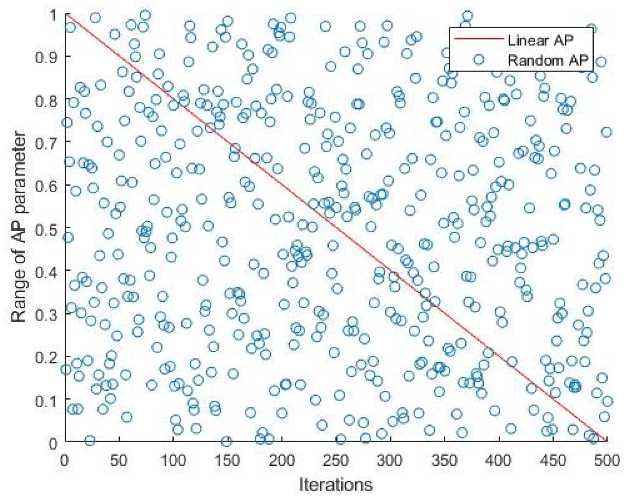
In the SFO, AP is a linearly decreasing parameter that is based on the parameter A and the convergence factor $ϵ$ (Equation (5)). It is clearly evident in Figure 1 as a straight line. When a sailfish attacks sardines (prey), they immediately disperse in different directions. Therefore, the sailfish should change the search direction to find the optimal solution. However, due to the linear AP parameter, the SFO does not address this random behavior of sardines. It is worth mentioning that AP is the main parameter for switching between exploration and exploitation. Therefore, the parameter needs improvement to align with the behavior of sardines. In the MSSFO, the AP is improved from a linear to a uniform random parameter within the range [0, 1], as shown in Figure 1 with circles. This promotes proper balance between exploration and exploitation and enables faster convergence towards the optimum value.

3.3.3. The Modified Hunting Process

Towards the last stage of the optimization process in the original SFO, if the injured sardine (the best sardine) is better than any of the sailfish, then the sardine is replaced with that sailfish in the candidate solution (represented by Equation (6)). This way, a sardine is hunted and hence removed from the sardine population. The problem with this technique is that the best sailfish already present in the candidate solution might be removed, and there is a chance that the algorithm gets stuck in a local optimum despite all the hunting process.

To address this limitation, the hunting mechanism has been modified by substituting an injured (best) sardine into the sailfish population if the worst solution in the sailfish population is also poorer than the best sardine. This avoids losing the best solutions in the sailfish population, and candidate solutions will be refined to have better positions in the search space. The modified hunting procedure is implemented using Equation (15):

$$X_{\mathrm{worst}\_\mathrm{SF}}=X_{\mathrm{injuredS}}\mathrm{if}fitness\left(X_{\mathrm{injuredS}}\right)<fitness\left(X_{\mathrm{worst}\_\mathrm{SF}}\right)$$

(15)

where $X_{\mathrm{worst}\_\mathrm{SF}}$ is the worst sailfish in the sailfish population and $X_{\mathrm{injuredS}}$ is the best sardine in the sardine population. If $X_{\mathrm{injuredS}}$ has a lower cost compared with $S{F}_{\mathrm{worst}}$ (i.e., the injured sardine is better than the worst sailfish), then the injured sardine is replaced with the worst sailfish and removed from the sardine population.

3.3.4. Dynamic Sardine Population

The purpose of having one more population (i.e. the sardine population) in the SFO is to prevent the algorithm from getting stuck in the local optima and to provide better exploration capabilities. It is also important to note that the sailfish position is updated based on the parameter $\lambda$, which further depends on prey density. In the original SFO, when the sardine population becomes zero, the global best position of the sailfish becomes fixed at that point, and no further improvement is possible. This leads to premature convergence.

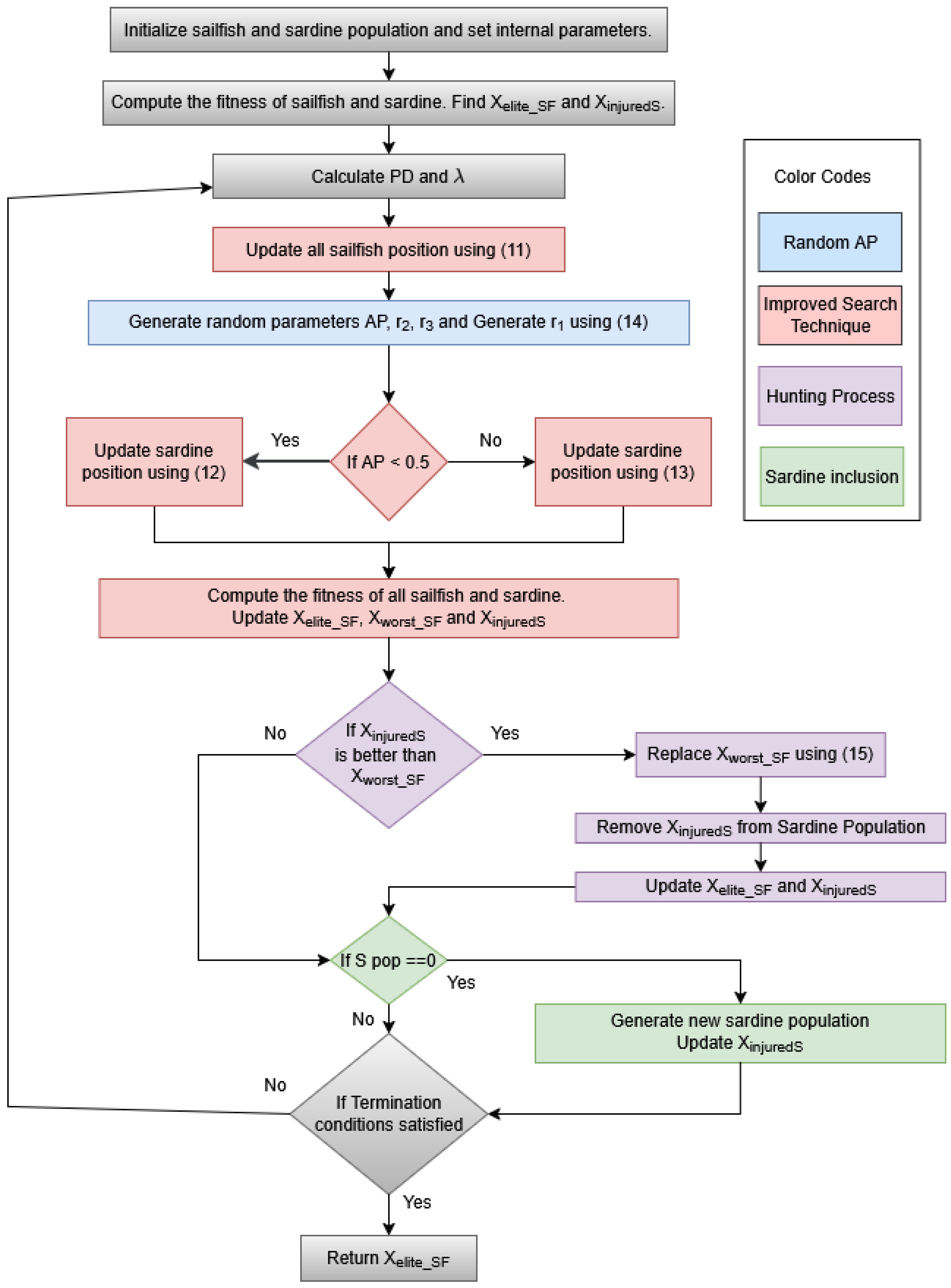
In this study, when all the sardines are either hunted or have run away from the search space, then sailfish will look for more sardines. In other words, when the sardine population becomes empty, more sardines are added to the sardine population. This is referred to as dynamic sardine population in this study and is employed when the sardine population becomes empty. Incorporating all the modifications, the MSSFO is presented in Algorithm 3, along with the flowchart in Figure 2.

3.3.5. Complexity of the Proposed Algorithm

In this section, the computational complexity of the MSSFO is discussed. Here, the number of sailfish is denoted by N, number of sardines is taken as M, and the dimensions are represented by D.

• Initialization of the sailfish and sardine takes $\mathcal{O}(N·D+M·D)$ time.
• To update the position of sailfish, $\mathcal{O}(N·D)$ time is needed.
• To update the position of sardine population, approximately $\mathcal{O}(M·D)$ time is required.

It is important to highlight that the MSSFO retains the same computational complexity as the original SFO. The modification strategies applied to improve the SFO do not alter its overall complexity. Therefore, the computational cost of the algorithm remains unchanged throughout the execution.

Algorithm 3 Proposed Multi-Strategy Sailfish Optimizer.

1: Initialize the population of sailfish and sardines randomly based on $PP=0.3$   2: Set parameters $a=2$, $\alpha =0.01$, $\beta =0.2$   3: Compute the fitness of sailfish and sardine solutions   4: Find the best sailfish and injured sardine   5: while termination conditions are not satisfied do   6:       Calculate $PD$ using Equation (3)   7:       for each sailfish do   8:             Calculate ${\lambda }_i$ using Equation (2)   9:             Update the position of sailfish using Equation (11) 10:       end for 11:       Generate $AP$, $r_2$, $r_3$ randomly within specified ranges 12:       Generate $r_1$ using Equation (14) 13:       if $AP<0.5$ then 14:             Update the position of sardine using Equation (12) 15:       else 16:             Update the position of sardine using Equation (13) 17:       end if 18:       Compute the fitness of sailfish and sardines using the objective function 19:       Update best sailfish, worst sailfish, and injured sardine 20:       if injured sardine is better than worst sailfish then 21:             Replace worst sailfish using Equation (15) 22:             Remove hunted sardine from the population 23:             Update best sailfish and injured sardine 24:       end if 25:       if sardine population is empty then 26:             Re-initialize sardine population 27:             Update injured sardine 28:       end if 29: end while 30: return best sailfish

4. Experimental Testing and Evaluation

This section is dedicated to the experimental evaluations and analysis. First, the experimental settings and the benchmark functions are discussed. This is followed by a discussion of results in terms of

• Parameter sensitivity analysis.
• Analysis of the proposed strategy.
• Comparative performance evaluation on benchmark functions.
• Statistical analysis.
• Performance evaluation on two real-world problems.

4.1. Experimental Setup and Benchmark Functions

Simulations are performed to observe and prove the significance of the MSSFO compared with the other metaheuristics employed in this study. All experiments are implemented in MATLAB R2019b with 64-bit Microsoft Windows 10, Intel(R) Core (TM) i5-11400 @ 2.60 Ghz, and 32 GB of RAM. CEC 2022 single-objective bound-constrained (SO-BO) numerical optimization problems [81] are employed to test the performance of the proposed MSSFO. The CEC 2022 SO-BO problems consist of twelve minimization functions divided into four categories: unimodal (F1), multimodal (F2–F5), hybrid (F6–F8), and composite functions (F9–F12). All the functions are executed 30 times on 10 and 20 dimensions with the Maximum Function Evaluations (MaxFEs) set to 200,000 and 1,000,000, respectively, and the error values [F(x) − F(x*)] are obtained for all the test problems. All the experimental settings are kept consistent as per the CEC 2022 SO-BO settings.

4.2. Parameter Sensitivity Analysis

In this section, a parameter sensitivity analysis is performed for parameters $\alpha$ and $\beta$ along with the exponentially decreasing parameter a. In the MSSFO, these parameters are used to find $r_1$, which is used to balance the exploration and exploitation processes. Two functions from each category of the CEC 2022 SO-BO are chosen (except the unimodal category because F1 is the only unimodal function) to perform this analysis, namely, F1, F2, F3, F6, F7, F11, and F12. The original source uses $\alpha$ = 0.03 and $\beta$ = 0.2 with a = 2 without providing a specific reason for the use of these values. Therefore, to verify the validity of the approach and to find the best combinations, experiments are run using different combinations of $\alpha$ and $\beta$ first, and then the top three combinations with the lowest mean error values [F(x) − F(x*)] are tested with three different values of the parameter a = 2, 3, and 4. Finally, the best combination of the set of values for all the parameters is chosen based on the results obtained.

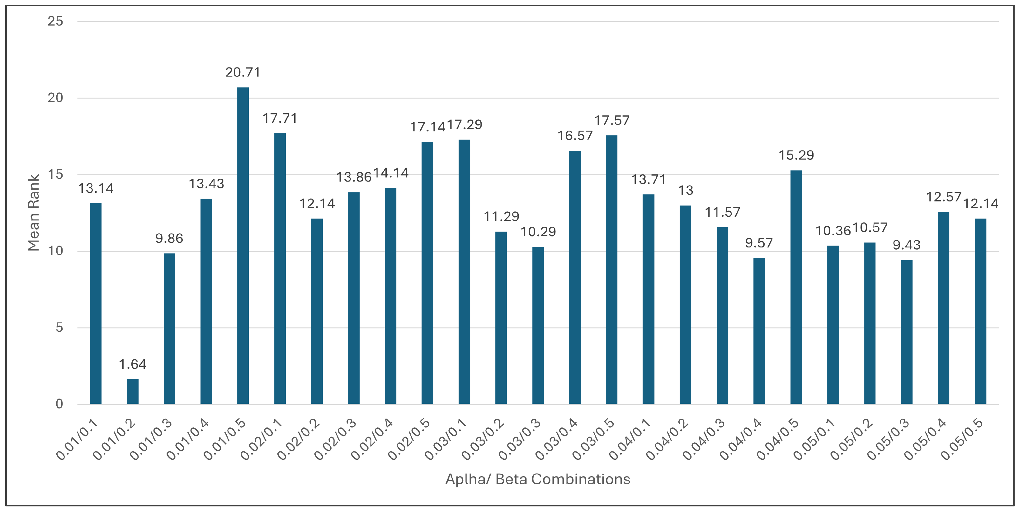
Parameter $\alpha$ ranges from 0.01 to 0.05, and parameter $\beta$ ranges from 0.1 to 0.5, making twenty-five combinations with both the parameters. Using these combinations, mean results for 30 independent runs are reported in

Table 2. Results of F1–F3 for different combinations of $\alpha$ and $\beta$.

		F1		F2		F3
$\mathit{\alpha }$	$\mathit{\beta }$	Avg	Rank	Avg	Rank	Avg	Rank
0.01	0.1	$6.6386\times {10}^{-8}$	6	$1.1699\times {10}^1$	9	$1.4805\times {10}^1$	25
	0.2	$0.0000\times {10}^0$	1.5	$7.3515\times {10}^0$	3	$9.1143\times {10}^0$	1
	0.3	$6.5874\times {10}^0$	19	$2.0029\times {10}^1$	18	$9.1990\times {10}^0$	3
	0.4	$1.0665\times {10}^4$	24	$1.7693\times {10}^2$	24	$9.8464\times {10}^0$	8
	0.5	$2.0577\times {10}^4$	25	$9.7362\times {10}^2$	25	$1.3235\times {10}^1$	24
0.02	0.1	$1.4822\times {10}^{-7}$	8	$1.4619\times {10}^1$	12	$1.2358\times {10}^1$	22
	0.2	$1.0529\times {10}^{-8}$	4	$1.5030\times {10}^1$	15	$1.2367\times {10}^1$	23
	0.3	$1.6868\times {10}^{-4}$	15	$1.9460\times {10}^1$	16	$9.8004\times {10}^0$	7
	0.4	$2.8618\times {10}^2$	21	$3.1422\times {10}^1$	21	$1.0632\times {10}^1$	11
	0.5	$9.3231\times {10}^3$	23	$1.1485\times {10}^2$	23	$1.0796\times {10}^1$	12
0.03	0.1	$1.5133\times {10}^{-7}$	9	$4.9968\times {10}^0$	1	$1.1919\times {10}^1$	18
	0.2	$6.3978\times {10}^{-8}$	5	$7.3503\times {10}^0$	2	$1.0989\times {10}^1$	14
	0.3	$2.2637\times {10}^{-7}$	10	$1.0080\times {10}^1$	7	$9.4864\times {10}^0$	5
	0.4	$9.8952\times {10}^{-3}$	17	$1.9895\times {10}^1$	17	$1.0553\times {10}^1$	10
	0.5	$2.1275\times {10}^3$	22	$3.8568\times {10}^1$	22	$1.2303\times {10}^1$	21
0.04	0.1	$6.8786\times {10}^{-9}$	3	$1.0605\times {10}^1$	8	$1.2005\times {10}^1$	19
	0.2	$2.3170\times {10}^{-7}$	11	$9.7312\times {10}^0$	6	$1.1108\times {10}^1$	16
	0.3	$1.0971\times {10}^{-7}$	7	$1.4404\times {10}^1$	11	$9.6357\times {10}^0$	6
	0.4	$2.4395\times {10}^{-4}$	16	$1.4981\times {10}^1$	14	$9.1159\times {10}^0$	2
	0.5	$7.3075\times {10}^0$	20	$2.4589\times {10}^1$	19	$9.2072\times {10}^0$	4
0.05	0.1	$0.0000\times {10}^0$	1.5	$1.4245\times {10}^1$	10	$1.0844\times {10}^1$	13
	0.2	$6.1100\times {10}^{-6}$	13	$9.4147\times {10}^0$	5	$1.2055\times {10}^1$	20
	0.3	$1.9883\times {10}^{-6}$	12	$9.1384\times {10}^0$	4	$1.0522\times {10}^1$	9
	0.4	$2.1489\times {10}^{-5}$	14	$1.4887\times {10}^1$	13	$1.1502\times {10}^1$	17
	0.5	$1.4956\times {10}^{-1}$	18	$2.7080\times {10}^1$	20	$1.1095\times {10}^1$	15

Note: Values highlighted in gray represent the best results.

and

Table 3. Results of F6-F7 and F11-F12 for different combinations of $\alpha$ and $\beta$.

		F6		F7		F11		F12
$\mathit{\alpha }$	$\mathit{\beta }$	Avg	Rank	Avg	Rank	Avg	Rank	Avg	Rank
0.01	0.1	$1.5653\times {10}^3$	12	$4.0530\times {10}^1$	14	$1.6284\times {10}^2$	25	$1.6482\times {10}^2$	1
	0.2	$1.1219\times {10}^3$	1	$3.5773\times {10}^1$	1	$5.1681\times {10}^1$	2	$1.6487\times {10}^2$	2
	0.3	$1.4805\times {10}^3$	6	$3.9062\times {10}^1$	9	$7.1588\times {10}^1$	5	$1.6537\times {10}^2$	9
	0.4	$1.6068\times {10}^3$	13	$3.6987\times {10}^1$	2	$6.9079\times {10}^1$	4	$1.6569\times {10}^2$	19
	0.5	$1.3525\times {10}^3$	3	$4.6178\times {10}^1$	25	$1.1906\times {10}^2$	20	$1.6592\times {10}^2$	23
0.02	0.1	$1.9647\times {10}^3$	21	$4.1815\times {10}^1$	17	$1.2807\times {10}^2$	22	$1.6577\times {10}^2$	22
	0.2	$1.8852\times {10}^3$	20	$3.8632\times {10}^1$	7	$6.2328\times {10}^1$	3	$1.6552\times {10}^2$	13
	0.3	$1.7815\times {10}^3$	19	$4.2817\times {10}^1$	19	$3.0588\times {10}^1$	1	$1.6574\times {10}^2$	20
	0.4	$1.7097\times {10}^3$	17	$3.7336\times {10}^1$	3	$9.4186\times {10}^1$	12	$1.6557\times {10}^2$	14
	0.5	$2.0522\times {10}^3$	23	$3.7783\times {10}^1$	5	$1.1678\times {10}^2$	19	$1.6557\times {10}^2$	15
0.03	0.1	$2.1016\times {10}^3$	24	$4.2843\times {10}^1$	20	$1.4338\times {10}^2$	24	$1.6714\times {10}^2$	25
	0.2	$1.5529\times {10}^3$	9	$4.3706\times {10}^1$	22	$1.1307\times {10}^2$	16	$1.6543\times {10}^2$	11
	0.3	$1.7032\times {10}^3$	16	$4.3825\times {10}^1$	23	$8.1911\times {10}^1$	8	$1.6500\times {10}^2$	3
	0.4	$1.7657\times {10}^3$	18	$4.4734\times {10}^1$	24	$8.4768\times {10}^1$	9	$1.6574\times {10}^2$	21
	0.5	$1.6508\times {10}^3$	14	$4.0891\times {10}^1$	15	$1.1938\times {10}^2$	21	$1.6534\times {10}^2$	8
0.04	0.1	$1.4633\times {10}^3$	5	$4.3571\times {10}^1$	21	$1.3339\times {10}^2$	23	$1.6565\times {10}^2$	17
	0.2	$1.5340\times {10}^3$	7	$4.2702\times {10}^1$	18	$1.1255\times {10}^2$	15	$1.6567\times {10}^2$	18
	0.3	$2.0100\times {10}^3$	22	$3.9717\times {10}^1$	12	$8.7831\times {10}^1$	11	$1.6544\times {10}^2$	12
	0.4	$1.5610\times {10}^3$	10	$3.8962\times {10}^1$	8	$8.7742\times {10}^1$	10	$1.6526\times {10}^2$	7
	0.5	$1.5622\times {10}^3$	11	$4.1371\times {10}^1$	16	$1.0816\times {10}^2$	13	$1.6607\times {10}^2$	24
0.05	0.1	$1.4348\times {10}^3$	4	$3.9656\times {10}^1$	11	$1.1485\times {10}^2$	17	$1.6562\times {10}^2$	16
	0.2	$1.2086\times {10}^3$	2	$3.7919\times {10}^1$	6	$1.1574\times {10}^2$	18	$1.6540\times {10}^2$	10
	0.3	$2.1855\times {10}^3$	25	$3.7618\times {10}^1$	4	$7.3165\times {10}^1$	6	$1.6525\times {10}^2$	6
	0.4	$1.6923\times {10}^3$	15	$3.9376\times {10}^1$	10	$1.1157\times {10}^2$	14	$1.6519\times {10}^2$	5
	0.5	$1.5442\times {10}^3$	8	$4.0060\times {10}^1$	13	$7.6264\times {10}^1$	7	$1.6513\times {10}^2$	4

Note: Values highlighted in gray represent the best results.

along with an individual ranking of each combination. It is interesting to note that the 0.01/0.2 combination is dominant in all the test problems, except F2 and F11. For both F2 and F11, the 0.01/0.2 combination is listed in the top three, making it a good choice for further experimentation. A mean rank based on the Friedman test is also computed and presented in Figure 3, where the superiority of the second combination (0.01/0.2) is clearly visible. Next, the experimentation is conducted to find the best value of parameter a with the top three combinations of $\alpha$ and $\beta$.

The top three combinations of $\alpha$/$\beta$ are 0.01/0.2, 0.04/0.4, and 0.05/0.3, as evident from Figure 3. The original source uses a value of 2 for the parameter a; hence, the values 2, 3, and 4 are used for this evaluation. The mean results of all the nine combinations are reported in

Table 4. Mean results for top three combinations from Figure 3 with different values of a.

Parameter a	$\mathit{\alpha },\mathit{\beta }$	F1	F2	F3	F6	F7	F11	F12
2	0.01, 0.2	$0.0000\times {10}^0$	$7.3515\times {10}^0$	$9.1143\times {10}^0$	$1.1219\times {10}^3$	$3.5773\times {10}^1$	$5.1681\times {10}^1$	$1.6487\times {10}^2$
3	0.01, 0.2	$1.4316\times {10}^{-4}$	$1.0520\times {10}^1$	$1.4401\times {10}^1$	$1.3445\times {10}^3$	$4.3822\times {10}^1$	$5.1903\times {10}^1$	$1.6628\times {10}^2$
4	0.01, 0.2	$1.5481\times {10}^{-6}$	$8.5955\times {10}^0$	$1.2741\times {10}^1$	$1.3761\times {10}^3$	$4.8739\times {10}^1$	$1.1726\times {10}^2$	$1.6555\times {10}^2$
2	0.04, 0.4	$2.4395\times {10}^{-4}$	$1.4981\times {10}^1$	$9.1159\times {10}^0$	$1.4911\times {10}^3$	$3.8962\times {10}^1$	$8.7742\times {10}^1$	$1.6526\times {10}^2$
3	0.04, 0.4	$4.4471\times {10}^{-3}$	$1.6519\times {10}^1$	$1.2924\times {10}^1$	$2.1332\times {10}^3$	$4.8526\times {10}^1$	$5.3347\times {10}^1$	$1.6674\times {10}^2$
4	0.04, 0.4	$1.0362\times {10}^{-2}$	$1.3194\times {10}^1$	$1.4388\times {10}^1$	$1.9223\times {10}^3$	$4.1522\times {10}^1$	$1.2788\times {10}^2$	$1.6622\times {10}^2$
2	0.05, 0.3	$1.9883\times {10}^{-6}$	$9.1384\times {10}^0$	$1.0522\times {10}^1$	$1.5946\times {10}^3$	$3.7618\times {10}^1$	$7.3165\times {10}^1$	$1.6525\times {10}^2$
3	0.05, 0.3	$1.9657\times {10}^{-2}$	$1.4837\times {10}^1$	$1.1758\times {10}^1$	$2.4062\times {10}^3$	$4.5720\times {10}^1$	$1.1643\times {10}^2$	$1.6631\times {10}^2$
4	0.05, 0.3	$8.7778\times {10}^{-2}$	$7.7199\times {10}^0$	$1.5210\times {10}^1$	$2.2510\times {10}^3$	$4.8176\times {10}^1$	$1.1237\times {10}^2$	$1.6611\times {10}^2$

Note: Values highlighted in gray represent the best results.

, where the best result is highlighted, which verifies the superiority of value 2 with the 0.01/0.2 combination of $\alpha$/$\beta$. Therefore, the final values of the parameters a, $\alpha$, and $\beta$ for further experiments are set to 2, 0.01, and 0.2, respectively.

4.3. Analysis of the Proposed Strategy

In this section, an analysis of the proposed improvement techniques is performed to find the impact of each strategy. Simulations are run using the CEC 2022 SO-BO functions (dim = 10) for this purpose. All the improvement techniques are applied to the SFO one by one to study the impact of each modification individually and collectively, reporting the mean error values along with the ranks presented in

Table 5. Comparison of the original SFO and its modified variants across 12 test functions. Numbers in parentheses represent the rank.

F	SFO	MSFO-A	MSFO-B	MSFO-C	MSFO-D	MSFO-AC	MSFO-AD	MSSFO
Test Function	Original	Modified Search Strategy	Random AP Parameter	Modified Hunting Technique	Dynamic Sardine Population	MSFO-A and MSFO-C Combined	MSFO-A and MSFO-D Combined	All Techniques Combined
1	$2.6163\times {10}^4$ (4)	$3.5154\times {10}^4$ (5)	$3.8178\times {10}^4$ (8)	$3.6665\times {10}^4$ (7)	$3.6644\times {10}^4$ (6)	$2.0103\times {10}^4$ (3)	$3.6491\times {10}^{-4}$ (2)	$0.0000\times {10}^0$ (1)
2	$9.9338\times {10}^2$ (7)	$5.3271\times {10}^2$ (4)	$9.2094\times {10}^2$ (6)	$1.1435\times {10}^3$ (8)	$6.8244\times {10}^2$ (5)	$2.1423\times {10}^2$ (3)	$1.5793\times {10}^1$ (2)	$7.3515\times {10}^0$ (1)
3	$6.2493\times {10}^1$ (5)	$7.0819\times {10}^1$ (8)	$6.4794\times {10}^1$ (6)	$7.0212\times {10}^1$ (7)	$5.4497\times {10}^1$ (3)	$5.5280\times {10}^1$ (4)	$1.2307\times {10}^1$ (2)	$9.1143\times {10}^0$ (1)
4	$8.1641\times {10}^1$ (6)	$8.6126\times {10}^1$ (7)	$7.2922\times {10}^1$ (4)	$9.5074\times {10}^1$ (8)	$7.7996\times {10}^1$ (5)	$6.5611\times {10}^1$ (3)	$3.2569\times {10}^1$ (2)	$2.0463\times {10}^1$ (1)
5	$1.2375\times {10}^3$ (5)	$1.5085\times {10}^3$ (7)	$1.4391\times {10}^3$ (6)	$1.7471\times {10}^3$ (8)	$7.8368\times {10}^2$ (4)	$7.4164\times {10}^2$ (3)	$8.8941\times {10}^0$ (2)	$3.6275\times {10}^{-1}$ (1)
6	$2.3658\times {10}^8$ (6)	$1.3652\times {10}^8$ (4)	$1.9521\times {10}^8$ (5)	$3.0914\times {10}^8$ (8)	$2.4086\times {10}^8$ (7)	$5.4424\times {10}^6$ (3)	$1.5912\times {10}^3$ (2)	$1.1219\times {10}^3$ (1)
7	$1.7343\times {10}^2$ (5)	$1.7665\times {10}^2$ (6)	$1.7917\times {10}^2$ (7)	$1.9100\times {10}^2$ (8)	$1.4060\times {10}^2$ (3)	$1.4145\times {10}^2$ (4)	$4.2933\times {10}^1$ (2)	$3.5773\times {10}^1$ (1)
8	$1.2375\times {10}^2$ (5)	$1.3864\times {10}^2$ (7)	$1.3211\times {10}^2$ (6)	$1.4663\times {10}^2$ (8)	$1.2109\times {10}^2$ (4)	$1.1304\times {10}^2$ (3)	$2.9527\times {10}^1$ (2)	$2.5802\times {10}^1$ (1)
9	$4.7218\times {10}^2$ (5)	$4.7919\times {10}^2$ (6)	$4.9568\times {10}^2$ (7)	$5.0672\times {10}^2$ (8)	$4.3381\times {10}^2$ (3)	$4.5286\times {10}^2$ (4)	$2.3529\times {10}^2$ (2)	$2.2930\times {10}^2$ (1)
10	$7.8722\times {10}^2$ (5)	$1.1059\times {10}^3$ (8)	$9.6408\times {10}^2$ (6)	$1.0234\times {10}^3$ (7)	$6.8686\times {10}^2$ (4)	$4.3610\times {10}^2$ (3)	$1.3343\times {10}^2$ (2)	$1.0545\times {10}^2$ (1)
11	$9.6630\times {10}^2$ (6)	$8.9888\times {10}^2$ (5)	$1.0446\times {10}^3$ (8)	$1.0230\times {10}^3$ (7)	$8.4426\times {10}^2$ (4)	$5.5028\times {10}^2$ (3)	$1.0522\times {10}^2$ (2)	$5.1681\times {10}^1$ (1)
12	$2.5415\times {10}^2$ (8)	$2.4837\times {10}^2$ (5)	$2.5253\times {10}^2$ (7)	$2.5223\times {10}^2$ (6)	$2.3693\times {10}^2$ (3)	$2.3738\times {10}^2$ (4)	$1.6599\times {10}^2$ (2)	$1.6487\times {10}^2$ (1)

.

First, the performance of the original SFO has been evaluated on all the test functions. Thereafter, individual improvements are applied to the SFO, named MSFO-A (Modified Search Strategy), MSFO-B (Random AP Parameter), MSFO-C (Modified Hunting Technique), and MSFO-D (Dynamic Sardine Population). The mean results from the 30 runs are reported in Table 5 along with the ranks reported within parenthesis. It is evident that the MSFO-A strategy shows better performance in F2, F6, F11, and F12 and the MSFO-B strategy is better in F2, F4, F6, and F12 compared with the SFO. Interestingly, the MSFO-C strategy does not have much impact on the SFO alone, except function F12, for which performance is improved. The MSFO-D strategy has the most significant impact on the performance of the SFO, and the results are evident in 9 out of the 12 problems, i.e., F2 to F5 and F7 to F12.

The combined effect of the modifications is then analyzed by integrating the MSFO-A strategy with the MSFO-C and MSFO-D strategies separately. Since the MSFO-A strategy already incorporates a randomized AP parameter, it is unnecessary to combine it with the MSFO-B strategy. The two combined variants, the MSFO-AC and the MSFO-AD strategies, are reported in Table 5. To statistically prove effectiveness, a Wilcoxon signed-rank test is also employed for the SFO vs. MSFO-AC and MSFO-AD strategies, giving a p-value less than the significance level (p < 0.05), which proves that both the combinations are significantly better than the SFO.

The final version of the improved SFO with all the strategies combined is termed the MSSFO, and the results are presented in the last column of Table 5. The MSSFO achieves the top rank by exhibiting top performance among all variants. To further analyze the significance of the MSSFO, a Wilcoxon signed-rank test is performed at a 95% significance level, which results in a p-value of less than 0.05. This validates that the MSSFO has significantly improved the SFO and can be further evaluated with the other optimization algorithms.

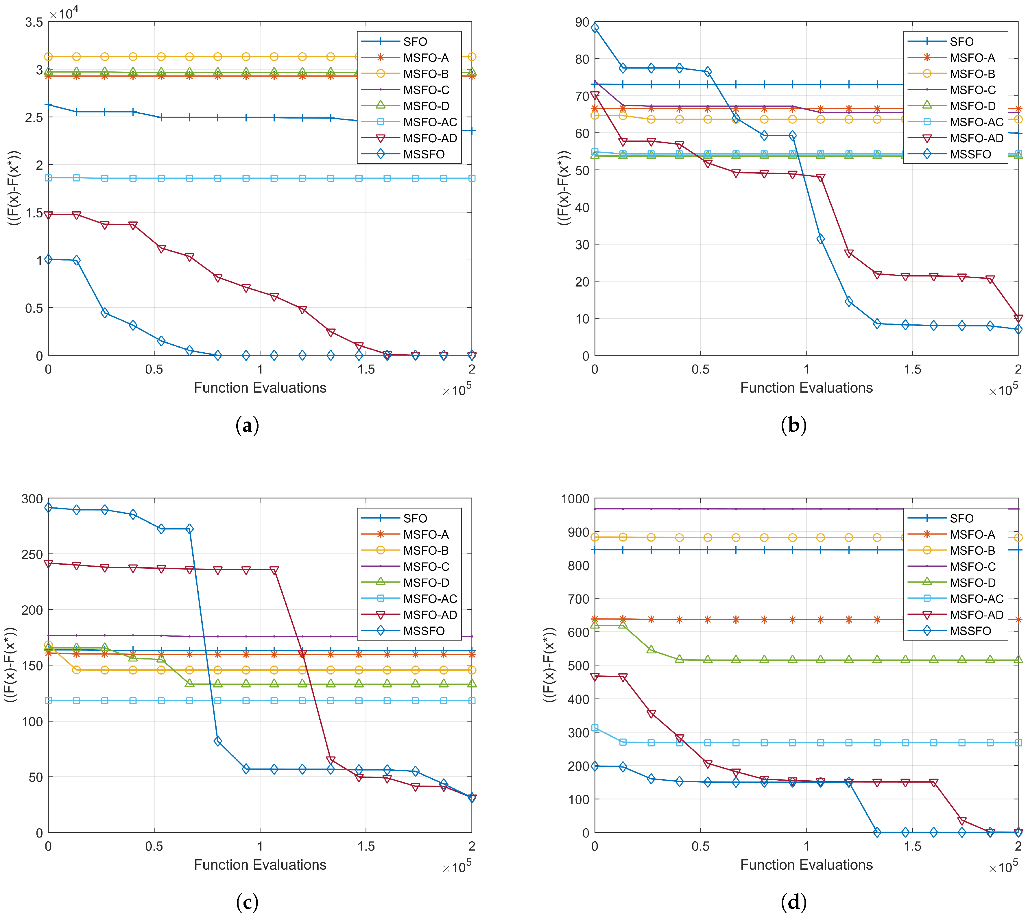
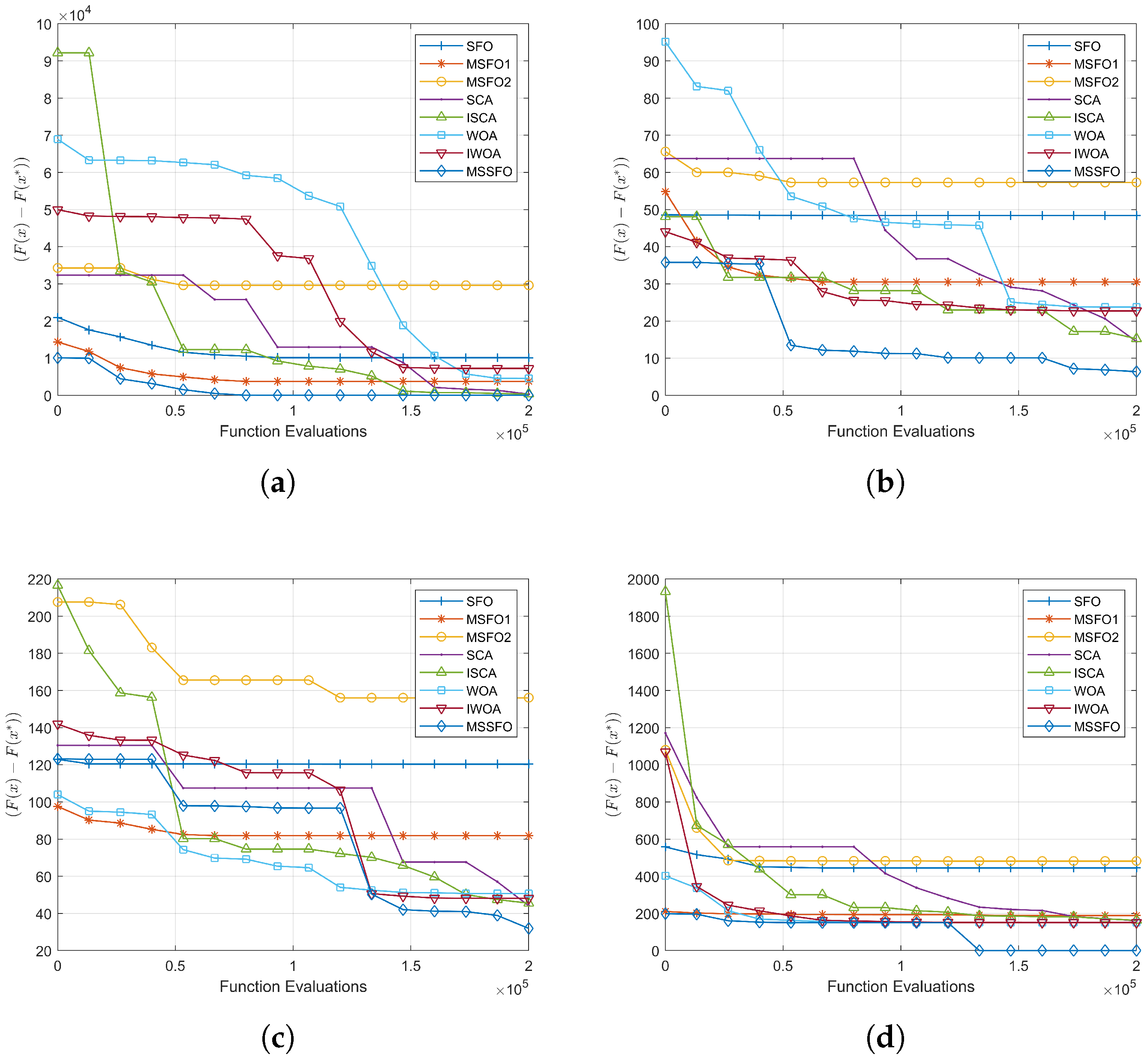
A convergence analysis for selected functions (F1, F3, F7, and F11) is also performed to show the superior convergence capabilities of the MSSFO, presented in Figure 4. One function from each category is used to visualize the convergence curve, including F1-unimodal, F3-multimodal, F7-Hybrid, and F11-composite functions. In all the problems, the MSSFO exhibits faster convergence and jumps out of the local optima quickly compared with the other variants. A similar trend can be observed in all the other functions.

4.4. Comparative Performance Evaluation on Benchmark Functions

In this section, the MSSFO is applied to solve the CEC 2022 SO-BO problems and compared with various well-known optimization algorithms, including the SFO, two other variants of the SFO (MSFO-1 [6] and MSFO-2 [8]), the SCA [23], the ISCA [34], the WOA [24], and the IWOA [38]. The basic and improved techniques for all the selected algorithms are used to give a better performance comparison. The SFO is used because it is the original algorithm on which the MSSFO is based, and the SCA and ISCA are compared because in the MSSFO, the SCA strategy is used to update the sardine position. The WOA is a well-established optimization algorithm; therefore, it is used along with an improved variant for performance comparison. The initial population is set to 30 for all the algorithms, as this size is typically used by researchers in similar studies [24,28]. The rest of the parameter settings of all the compared algorithms are consistent with the original papers and are presented in

Table 6. Parameter settings for compared algorithms.

Algorithm	Parameter	Value
SFO	PP	0.3
	Convergence parameter (A)	4
	Convergence factor ($\epsilon$)	0.0001
WOA	a	Linearly decreases from 2 to 0
SCA	a	2

.

All the experimental settings for this experimentation follow the guidelines of the CEC 2022 SO-BO. The simulations are performed for 10 and 20 dimensions with 30 runs per problem. The MaxFEs are set to 200,000 and 1,000,000 for the 10- and 20-dimensional problems, respectively. Error values (calculated value minus optimal value) are obtained from each run for all the problems on both the dimensions. The mean, median, standard deviation, and best and worst results are presented in

Table 7. The results of utilized algorithms on CEC 2022 test suites with dim = 10.

	Func.	SFO	MSFO1	MSFO2	SCA	ISCA	WOA	IWOA	MSSFO
Best	1	$3.1112\times {10}^3$	$2.0028\times {10}^2$	$8.1724\times {10}^3$	$1.4113\times {10}^2$	$1.9956\times {10}^2$	$4.4335\times {10}^2$	$2.2715\times {10}^3$	$0.0000\times {10}^0$
Worst		$1.0466\times {10}^4$	$1.1183\times {10}^4$	$8.1323\times {10}^4$	$1.3955\times {10}^3$	$3.9493\times {10}^3$	$1.3986\times {10}^4$	$1.4241\times {10}^4$	$0.0000\times {10}^0$
Median		$1.0148\times {10}^4$	$3.9050\times {10}^3$	$3.0528\times {10}^4$	$3.4154\times {10}^2$	$4.0944\times {10}^2$	$4.7598\times {10}^3$	$7.4893\times {10}^3$	$0.0000\times {10}^0$
Mean		$9.4734\times {10}^3$	$4.5180\times {10}^3$	$3.2221\times {10}^4$	$3.9230\times {10}^2$	$5.6366\times {10}^2$	$5.2550\times {10}^3$	$7.5203\times {10}^3$	$0.0000\times {10}^0$
Std.		$1.5816\times {10}^3$	$2.8355\times {10}^3$	$1.7970\times {10}^4$	$2.4691\times {10}^2$	$6.7489\times {10}^2$	$2.8038\times {10}^3$	$3.3782\times {10}^3$	$0.0000\times {10}^0$
Best	2	$4.5811\times {10}^1$	$1.6249\times {10}^1$	$7.8909\times {10}^1$	$2.1475\times {10}^1$	$1.7492\times {10}^1$	$5.3500\times {10}^{-2}$	$1.1764\times {10}^{-1}$	$7.9166\times {10}^{-4}$
Worst		$7.2268\times {10}^2$	$3.9727\times {10}^2$	$1.5447\times {10}^3$	$6.6718\times {10}^1$	$6.4380\times {10}^1$	$9.2519\times {10}^1$	$9.7591\times {10}^1$	$7.6067\times {10}^1$
Median		$2.4825\times {10}^2$	$7.5646\times {10}^1$	$2.8871\times {10}^2$	$4.0092\times {10}^1$	$3.5439\times {10}^1$	$8.9169\times {10}^0$	$8.5089\times {10}^0$	$4.9552\times {10}^0$
Mean		$2.7381\times {10}^2$	$9.3971\times {10}^1$	$4.2051\times {10}^2$	$4.3054\times {10}^1$	$3.9423\times {10}^1$	$2.6935\times {10}^1$	$2.1280\times {10}^1$	$7.3515\times {10}^0$
Std		$1.6788\times {10}^2$	$9.2479\times {10}^1$	$3.5809\times {10}^2$	$1.4520\times {10}^1$	$1.2821\times {10}^1$	$3.3593\times {10}^1$	$2.8409\times {10}^1$	$1.3275\times {10}^1$
Best	3	$1.7260\times {10}^1$	$6.6521\times {10}^0$	$3.6954\times {10}^1$	$7.8270\times {10}^0$	$1.1126\times {10}^1$	$1.0266\times {10}^1$	$7.7087\times {10}^0$	$1.2031\times {10}^0$
Worst		$9.1782\times {10}^1$	$5.7124\times {10}^1$	$9.4189\times {10}^1$	$2.2915\times {10}^1$	$2.3835\times {10}^1$	$5.8677\times {10}^1$	$4.8530\times {10}^1$	$2.1961\times {10}^1$
Median		$5.1341\times {10}^1$	$3.6442\times {10}^1$	$5.8833\times {10}^1$	$1.4922\times {10}^1$	$1.5584\times {10}^1$	$2.5239\times {10}^1$	$2.3219\times {10}^1$	$7.6371\times {10}^0$
Mean		$4.9999\times {10}^1$	$3.1812\times {10}^1$	$6.0828\times {10}^1$	$1.4653\times {10}^1$	$1.6068\times {10}^1$	$2.8396\times {10}^1$	$2.4460\times {10}^1$	$9.1143\times {10}^0$
Std.		$1.7855\times {10}^1$	$1.3294\times {10}^1$	$1.4557\times {10}^1$	$3.1440\times {10}^0$	$2.7829\times {10}^0$	$1.1357\times {10}^1$	$1.0435\times {10}^1$	$5.1938\times {10}^0$
Best	4	$2.7512\times {10}^1$	$1.3234\times {10}^1$	$3.0532\times {10}^1$	$2.0718\times {10}^1$	$2.2784\times {10}^1$	$1.1941\times {10}^1$	$5.9754\times {10}^0$	$4.9748\times {10}^0$
Worst		$8.7690\times {10}^1$	$6.6593\times {10}^1$	$9.0641\times {10}^1$	$4.7732\times {10}^1$	$4.1864\times {10}^1$	$8.9546\times {10}^1$	$8.9548\times {10}^1$	$3.4823\times {10}^1$
Median		$5.4583\times {10}^1$	$2.8026\times {10}^1$	$6.6227\times {10}^1$	$3.1073\times {10}^1$	$3.1685\times {10}^1$	$3.7314\times {10}^1$	$3.6317\times {10}^1$	$2.1392\times {10}^1$
Mean		$5.6290\times {10}^1$	$2.9891\times {10}^1$	$6.7321\times {10}^1$	$3.1539\times {10}^1$	$3.1276\times {10}^1$	$3.8578\times {10}^1$	$3.7613\times {10}^1$	$2.0463\times {10}^1$
Std.		$1.4388\times {10}^1$	$1.0873\times {10}^1$	$1.2876\times {10}^1$	$6.4646\times {10}^0$	$4.4810\times {10}^0$	$1.5247\times {10}^1$	$1.6478\times {10}^1$	$6.6431\times {10}^0$
Best	5	$1.8725\times {10}^2$	$2.7617\times {10}^1$	$3.7696\times {10}^2$	$1.4395\times {10}^1$	$1.6963\times {10}^1$	$1.0114\times {10}^2$	$5.6183\times {10}^1$	$7.0950\times {10}^{-6}$
Worst		$1.4093\times {10}^3$	$9.9252\times {10}^2$	$2.4508\times {10}^3$	$1.3907\times {10}^2$	$1.9761\times {10}^2$	$1.4192\times {10}^3$	$1.2206\times {10}^3$	$1.8177\times {10}^0$
Median		$6.4946\times {10}^2$	$3.3180\times {10}^2$	$7.6033\times {10}^2$	$4.4918\times {10}^1$	$5.6693\times {10}^1$	$3.7064\times {10}^2$	$3.1161\times {10}^2$	$1.3447\times {10}^{-1}$
Mean		$7.0498\times {10}^2$	$3.7509\times {10}^2$	$8.9577\times {10}^2$	$5.0827\times {10}^1$	$6.1942\times {10}^1$	$4.3698\times {10}^2$	$3.9662\times {10}^2$	$3.6275\times {10}^{-1}$
Std.		$3.4210\times {10}^2$	$2.1513\times {10}^2$	$4.5273\times {10}^2$	$3.0218\times {10}^1$	$3.6613\times {10}^1$	$2.9928\times {10}^2$	$2.6007\times {10}^2$	$4.2561\times {10}^{-1}$
Best	6	$2.3032\times {10}^3$	$3.5453\times {10}^2$	$2.7537\times {10}^4$	$7.1650\times {10}^4$	$5.1363\times {10}^4$	$1.4430\times {10}^2$	$1.1082\times {10}^2$	$1.0117\times {10}^2$
Worst		$5.3373\times {10}^7$	$6.4910\times {10}^3$	$3.2238\times {10}^8$	$4.3103\times {10}^6$	$2.0638\times {10}^6$	$6.3453\times {10}^3$	$6.2977\times {10}^3$	$3.5740\times {10}^3$
Median		$5.5233\times {10}^5$	$1.8812\times {10}^3$	$9.4941\times {10}^6$	$5.1273\times {10}^5$	$5.4777\times {10}^5$	$1.1608\times {10}^3$	$8.5510\times {10}^2$	$6.7390\times {10}^2$
Mean		$6.5601\times {10}^6$	$2.3311\times {10}^3$	$4.4071\times {10}^7$	$8.7380\times {10}^5$	$6.8474\times {10}^5$	$1.8973\times {10}^3$	$1.5660\times {10}^3$	$1.1219\times {10}^3$
Std.		$1.3693\times {10}^7$	$1.9078\times {10}^3$	$8.0660\times {10}^7$	$8.8073\times {10}^5$	$5.0380\times {10}^5$	$1.8918\times {10}^3$	$1.5659\times {10}^3$	$1.0712\times {10}^3$
Best	7	$6.3844\times {10}^1$	$4.2106\times {10}^1$	$6.6883\times {10}^1$	$3.4702\times {10}^1$	$3.4877\times {10}^1$	$2.5160\times {10}^1$	$2.3967\times {10}^1$	$2.1158\times {10}^1$
Worst		$3.7723\times {10}^2$	$2.3858\times {10}^2$	$3.2251\times {10}^2$	$5.9795\times {10}^1$	$7.0241\times {10}^1$	$8.5812\times {10}^1$	$1.2074\times {10}^2$	$6.6095\times {10}^1$
Median		$1.2745\times {10}^2$	$9.2575\times {10}^1$	$1.6535\times {10}^2$	$4.4507\times {10}^1$	$4.5670\times {10}^1$	$5.1682\times {10}^1$	$5.1386\times {10}^1$	$3.2768\times {10}^1$
Mean		$1.4497\times {10}^2$	$9.8453\times {10}^1$	$1.7682\times {10}^2$	$4.5463\times {10}^1$	$4.9019\times {10}^1$	$5.4640\times {10}^1$	$5.5589\times {10}^1$	$3.5773\times {10}^1$
Std.		$6.2784\times {10}^1$	$4.7794\times {10}^1$	$6.5254\times {10}^1$	$5.3851\times {10}^0$	$8.5996\times {10}^0$	$1.6217\times {10}^1$	$2.2751\times {10}^1$	$1.1103\times {10}^1$
Best	8	$2.8076\times {10}^1$	$2.3269\times {10}^1$	$4.0190\times {10}^1$	$2.3761\times {10}^1$	$2.3128\times {10}^1$	$1.9611\times {10}^1$	$1.1913\times {10}^1$	$3.6426\times {10}^0$
Worst		$2.6165\times {10}^2$	$1.6464\times {10}^2$	$3.7516\times {10}^2$	$3.2769\times {10}^1$	$3.4385\times {10}^1$	$4.3236\times {10}^1$	$4.4081\times {10}^1$	$3.5542\times {10}^1$
Median		$7.0587\times {10}^1$	$4.3154\times {10}^1$	$1.2803\times {10}^2$	$2.9680\times {10}^1$	$2.9449\times {10}^1$	$3.0820\times {10}^1$	$3.0541\times {10}^1$	$2.6217\times {10}^1$
Mean		$9.6254\times {10}^1$	$7.8773\times {10}^1$	$1.3496\times {10}^2$	$2.9284\times {10}^1$	$2.9404\times {10}^1$	$3.1491\times {10}^1$	$3.0543\times {10}^1$	$2.5802\times {10}^1$
Std.		$6.3497\times {10}^1$	$5.6069\times {10}^1$	$7.9203\times {10}^1$	$2.1213\times {10}^0$	$2.4960\times {10}^0$	$5.8880\times {10}^0$	$6.2490\times {10}^0$	$6.5687\times {10}^0$
Best	9	$3.0685\times {10}^2$	$2.3128\times {10}^2$	$3.0678\times {10}^2$	$2.3512\times {10}^2$	$2.3597\times {10}^2$	$2.2929\times {10}^2$	$2.2929\times {10}^2$	$2.2928\times {10}^2$
Worst		$5.0785\times {10}^2$	$4.7505\times {10}^2$	$7.5581\times {10}^2$	$2.7088\times {10}^2$	$2.8941\times {10}^2$	$3.7622\times {10}^2$	$2.8510\times {10}^2$	$2.2933\times {10}^2$
Median		$4.4218\times {10}^2$	$3.5607\times {10}^2$	$4.5840\times {10}^2$	$2.4781\times {10}^2$	$2.5453\times {10}^2$	$2.2937\times {10}^2$	$2.2934\times {10}^2$	$2.2929\times {10}^2$
Mean		$4.3408\times {10}^2$	$3.4517\times {10}^2$	$4.9056\times {10}^2$	$2.4856\times {10}^2$	$2.5759\times {10}^2$	$2.3800\times {10}^2$	$2.3748\times {10}^2$	$2.2930\times {10}^2$
Std.		$5.0937\times {10}^1$	$5.9495\times {10}^1$	$1.1079\times {10}^2$	$8.1763\times {10}^0$	$1.7699\times {10}^1$	$2.9119\times {10}^1$	$1.8907\times {10}^1$	$1.5923\times {10}^{-2}$
Best	10	$1.0067\times {10}^2$	$1.0056\times {10}^2$	$1.0554\times {10}^2$	$1.0081\times {10}^2$	$1.0080\times {10}^2$	$1.0031\times {10}^2$	$1.0040\times {10}^2$	$1.0047\times {10}^2$
Worst		$1.9875\times {10}^3$	$1.5189\times {10}^3$	$1.9705\times {10}^3$	$1.0536\times {10}^2$	$2.4260\times {10}^2$	$2.4679\times {10}^2$	$2.4729\times {10}^2$	$2.2873\times {10}^2$
Median		$2.4902\times {10}^2$	$2.3197\times {10}^2$	$2.7244\times {10}^2$	$1.0136\times {10}^2$	$1.0148\times {10}^2$	$1.0074\times {10}^2$	$1.0083\times {10}^2$	$1.0116\times {10}^2$
Mean		$4.0354\times {10}^2$	$3.2865\times {10}^2$	$5.0434\times {10}^2$	$1.0151\times {10}^2$	$1.3285\times {10}^2$	$1.4338\times {10}^2$	$1.3793\times {10}^2$	$1.0545\times {10}^2$
Std.		$5.0860\times {10}^2$	$4.0581\times {10}^2$	$5.9561\times {10}^2$	$7.8343\times {10}^{-1}$	$5.7174\times {10}^1$	$6.0623\times {10}^1$	$5.7132\times {10}^1$	$2.2901\times {10}^1$
Best	11	$2.1954\times {10}^2$	$1.0148\times {10}^2$	$2.0806\times {10}^2$	$1.3208\times {10}^2$	$1.5100\times {10}^2$	$5.1058\times {10}^{-1}$	$6.9950\times {10}^{-1}$	$0.0000\times {10}^0$
Worst		$2.1551\times {10}^3$	$1.3039\times {10}^3$	$1.7796\times {10}^3$	$1.7302\times {10}^2$	$5.4487\times {10}^2$	$6.2817\times {10}^2$	$6.2871\times {10}^2$	$4.0000\times {10}^2$
Median		$5.2141\times {10}^2$	$2.2664\times {10}^2$	$5.4017\times {10}^2$	$1.6178\times {10}^2$	$1.6315\times {10}^2$	$1.5094\times {10}^2$	$1.5110\times {10}^2$	$0.0000\times {10}^0$
Mean		$6.8545\times {10}^2$	$3.5514\times {10}^2$	$6.3216\times {10}^2$	$1.6057\times {10}^2$	$1.7607\times {10}^2$	$1.9771\times {10}^2$	$1.8582\times {10}^2$	$5.1681\times {10}^1$
Std.		$4.4805\times {10}^2$	$2.7022\times {10}^2$	$3.8154\times {10}^2$	$7.8473\times {10}^0$	$6.8683\times {10}^1$	$1.7882\times {10}^2$	$1.6552\times {10}^2$	$1.2145\times {10}^2$
Best	12	$1.6850\times {10}^2$	$1.6486\times {10}^2$	$1.6783\times {10}^2$	$1.6557\times {10}^2$	$1.6517\times {10}^2$	$1.6372\times {10}^2$	$1.6140\times {10}^2$	$1.6285\times {10}^2$
Worst		$3.2758\times {10}^2$	$2.7652\times {10}^2$	$3.0532\times {10}^2$	$1.7033\times {10}^2$	$1.9065\times {10}^2$	$2.3720\times {10}^2$	$2.3853\times {10}^2$	$1.6791\times {10}^2$
Median		$2.1911\times {10}^2$	$1.7433\times {10}^2$	$2.2802\times {10}^2$	$1.6764\times {10}^2$	$1.6759\times {10}^2$	$1.7224\times {10}^2$	$1.6962\times {10}^2$	$1.6494\times {10}^2$
Mean		$2.2552\times {10}^2$	$1.9148\times {10}^2$	$2.2284\times {10}^2$	$1.6772\times {10}^2$	$1.6815\times {10}^2$	$1.8182\times {10}^2$	$1.7663\times {10}^2$	$1.6487\times {10}^2$
Std.		$4.5750\times {10}^1$	$2.8811\times {10}^1$	$3.7813\times {10}^1$	$1.2837\times {10}^0$	$4.2585\times {10}^0$	$2.1797\times {10}^1$	$1.9711\times {10}^1$	$1.0370\times {10}^0$

Note: Values highlighted in gray represent the best results.

and

Table 8. The results of different algorithms on CEC 2022 test suite with dim = 20.

	Func.	SFO	MSFO1	MSFO2	SCA	ISCA	WOA	IWOA	MSSFO
Best	1	$3.7293\times {10}^4$	$9.8810\times {10}^3$	$5.2651\times {10}^4$	$2.1041\times {10}^3$	$2.1712\times {10}^3$	$1.6633\times {10}^0$	$1.8143\times {10}^3$	$3.0932\times {10}^{-3}$
Worst		$9.4503\times {10}^4$	$7.5677\times {10}^4$	$1.8301\times {10}^5$	$9.7667\times {10}^3$	$8.0624\times {10}^3$	$7.2329\times {10}^1$	$3.6010\times {10}^4$	$1.3539\times {10}^{-2}$
Median		$6.1895\times {10}^4$	$2.7820\times {10}^4$	$9.0587\times {10}^4$	$4.7091\times {10}^3$	$5.0153\times {10}^3$	$1.1429\times {10}^1$	$8.7585\times {10}^3$	$6.1565\times {10}^{-3}$
Mean		$6.2829\times {10}^4$	$3.1312\times {10}^4$	$1.0184\times {10}^5$	$5.3356\times {10}^3$	$5.2665\times {10}^3$	$2.1699\times {10}^1$	$9.3791\times {10}^3$	$6.7114\times {10}^{-3}$
Std.		$1.3326\times {10}^4$	$1.3139\times {10}^4$	$3.3626\times {10}^4$	$2.1205\times {10}^3$	$1.4064\times {10}^3$	$1.9790\times {10}^1$	$6.6195\times {10}^3$	$2.8183\times {10}^{-3}$
Best	2	$5.0222\times {10}^2$	$2.6535\times {10}^2$	$5.1638\times {10}^2$	$1.3096\times {10}^2$	$1.2702\times {10}^2$	$5.2450\times {10}^0$	$7.0481\times {10}^0$	$4.1375\times {10}^0$
Worst		$2.6767\times {10}^3$	$8.5071\times {10}^2$	$3.6395\times {10}^3$	$3.1774\times {10}^2$	$3.0106\times {10}^2$	$1.3216\times {10}^2$	$1.7209\times {10}^2$	$7.3867\times {10}^1$
Median		$1.2529\times {10}^3$	$4.7642\times {10}^2$	$1.7853\times {10}^3$	$1.8110\times {10}^2$	$1.8647\times {10}^2$	$4.9203\times {10}^1$	$6.5788\times {10}^1$	$4.9090\times {10}^1$
Mean		$1.3730\times {10}^3$	$4.7838\times {10}^2$	$1.9244\times {10}^3$	$1.9012\times {10}^2$	$1.9249\times {10}^2$	$5.8233\times {10}^1$	$8.3150\times {10}^1$	$4.8277\times {10}^1$
Std.		$5.5179\times {10}^2$	$1.3741\times {10}^2$	$7.2439\times {10}^2$	$4.2703\times {10}^1$	$3.2660\times {10}^1$	$2.0208\times {10}^1$	$4.5183\times {10}^1$	$1.6892\times {10}^1$
Best	3	$5.4917\times {10}^1$	$3.3641\times {10}^1$	$5.2358\times {10}^1$	$2.2928\times {10}^1$	$2.7114\times {10}^1$	$2.5098\times {10}^1$	$3.5982\times {10}^1$	$1.8164\times {10}^1$
Worst		$1.0601\times {10}^2$	$9.3314\times {10}^1$	$1.3581\times {10}^2$	$3.8717\times {10}^1$	$4.4901\times {10}^1$	$8.0737\times {10}^1$	$7.7349\times {10}^1$	$6.7681\times {10}^1$
Median		$7.8495\times {10}^1$	$5.7476\times {10}^1$	$9.3921\times {10}^1$	$3.0721\times {10}^1$	$3.1037\times {10}^1$	$5.1420\times {10}^1$	$5.3473\times {10}^1$	$4.8746\times {10}^1$
Mean		$7.9970\times {10}^1$	$5.9389\times {10}^1$	$9.3991\times {10}^1$	$3.0864\times {10}^1$	$3.2683\times {10}^1$	$5.4247\times {10}^1$	$5.4869\times {10}^1$	$4.8712\times {10}^1$
Std.		$1.3194\times {10}^1$	$1.5066\times {10}^1$	$1.7054\times {10}^1$	$3.8135\times {10}^0$	$4.3897\times {10}^0$	$1.0349\times {10}^1$	$9.5353\times {10}^0$	$1.2209\times {10}^1$
Best	4	$1.2502\times {10}^2$	$8.4397\times {10}^1$	$1.4900\times {10}^2$	$9.6359\times {10}^1$	$9.6206\times {10}^1$	$5.0743\times {10}^1$	$6.6665\times {10}^1$	$4.8753\times {10}^1$
Worst		$2.2570\times {10}^2$	$1.5740\times {10}^2$	$2.6506\times {10}^2$	$1.3240\times {10}^2$	$1.3374\times {10}^2$	$1.9402\times {10}^2$	$1.9402\times {10}^2$	$1.3332\times {10}^2$
Median		$1.7970\times {10}^2$	$1.2462\times {10}^2$	$1.9609\times {10}^2$	$1.1994\times {10}^2$	$1.1424\times {10}^2$	$1.0795\times {10}^2$	$1.0049\times {10}^2$	$7.6612\times {10}^1$
Mean		$1.8200\times {10}^2$	$1.2203\times {10}^2$	$1.9325\times {10}^2$	$1.1889\times {10}^2$	$1.1285\times {10}^2$	$1.1240\times {10}^2$	$1.1092\times {10}^2$	$7.7607\times {10}^1$
Std.		$2.5016\times {10}^1$	$2.0511\times {10}^1$	$2.5933\times {10}^1$	$8.4399\times {10}^0$	$9.4536\times {10}^0$	$3.3278\times {10}^1$	$3.5591\times {10}^1$	$1.8310\times {10}^1$
Best	5	$2.1957\times {10}^3$	$1.0196\times {10}^3$	$2.6940\times {10}^3$	$4.2817\times {10}^2$	$4.1414\times {10}^2$	$7.6928\times {10}^2$	$5.7352\times {10}^2$	$3.9719\times {10}^2$
Worst		$5.1042\times {10}^3$	$3.1661\times {10}^3$	$9.0338\times {10}^3$	$1.1778\times {10}^3$	$1.3208\times {10}^3$	$6.0255\times {10}^3$	$4.8438\times {10}^3$	$2.0443\times {10}^3$
Median		$3.2329\times {10}^3$	$2.1182\times {10}^3$	$3.9763\times {10}^3$	$6.6459\times {10}^2$	$6.7760\times {10}^2$	$1.7427\times {10}^3$	$1.5859\times {10}^3$	$1.2821\times {10}^3$
Mean		$3.2890\times {10}^3$	$2.1534\times {10}^3$	$4.1722\times {10}^3$	$7.0466\times {10}^2$	$7.4552\times {10}^2$	$2.1463\times {10}^3$	$1.8227\times {10}^3$	$1.2696\times {10}^3$
Std.		$7.1094\times {10}^2$	$4.5235\times {10}^2$	$1.2238\times {10}^3$	$1.9172\times {10}^2$	$2.2563\times {10}^2$	$1.1883\times {10}^3$	$9.2280\times {10}^2$	$3.5878\times {10}^2$
Best	6	$2.2958\times {10}^7$	$2.0585\times {10}^5$	$1.0181\times {10}^8$	$3.8309\times {10}^6$	$3.1969\times {10}^6$	$1.8848\times {10}^2$	$1.6012\times {10}^3$	$1.5133\times {10}^2$
Worst		$2.3583\times {10}^9$	$3.7976\times {10}^8$	$2.5228\times {10}^9$	$1.0917\times {10}^8$	$8.6440\times {10}^7$	$1.8672\times {10}^4$	$2.8832\times {10}^7$	$1.8597\times {10}^4$
Median		$5.5534\times {10}^8$	$1.5998\times {10}^7$	$7.2025\times {10}^8$	$4.8540\times {10}^7$	$1.8407\times {10}^7$	$3.3104\times {10}^3$	$1.8445\times {10}^5$	$2.1276\times {10}^3$
Mean		$7.4108\times {10}^8$	$3.0074\times {10}^7$	$8.7831\times {10}^8$	$4.6179\times {10}^7$	$2.5504\times {10}^7$	$5.2912\times {10}^3$	$3.1671\times {10}^6$	$4.1926\times {10}^3$
Std.		$6.1230\times {10}^8$	$6.6807\times {10}^7$	$6.2903\times {10}^8$	$2.7474\times {10}^7$	$2.1917\times {10}^7$	$5.3669\times {10}^3$	$7.1001\times {10}^6$	$4.4813\times {10}^3$
Best	7	$1.5841\times {10}^2$	$7.5627\times {10}^1$	$1.8871\times {10}^2$	$6.7648\times {10}^1$	$7.1328\times {10}^1$	$7.9205\times {10}^1$	$4.6775\times {10}^1$	$7.2849\times {10}^1$
Worst		$4.7869\times {10}^2$	$4.2448\times {10}^2$	$6.4841\times {10}^2$	$1.3355\times {10}^2$	$1.3126\times {10}^2$	$3.1242\times {10}^2$	$2.5819\times {10}^2$	$2.1709\times {10}^2$
Median		$2.8310\times {10}^2$	$2.0606\times {10}^2$	$3.6929\times {10}^2$	$9.4172\times {10}^1$	$1.0635\times {10}^2$	$1.5842\times {10}^2$	$1.4619\times {10}^2$	$1.2619\times {10}^2$
Mean		$2.8496\times {10}^2$	$2.2408\times {10}^2$	$3.6688\times {10}^2$	$9.3684\times {10}^1$	$1.0439\times {10}^2$	$1.5533\times {10}^2$	$1.4230\times {10}^2$	$1.2731\times {10}^2$
Std.		$8.2863\times {10}^1$	$8.8401\times {10}^1$	$1.0009\times {10}^2$	$1.3277\times {10}^1$	$1.3934\times {10}^1$	$5.1887\times {10}^1$	$5.0619\times {10}^1$	$3.6106\times {10}^1$
Best	8	$7.2435\times {10}^1$	$3.0949\times {10}^1$	$8.1869\times {10}^1$	$3.4470\times {10}^1$	$3.3475\times {10}^1$	$2.6779\times {10}^1$	$2.9448\times {10}^1$	$2.6091\times {10}^1$
Worst		$7.4573\times {10}^2$	$4.6507\times {10}^2$	$1.3551\times {10}^3$	$5.2388\times {10}^1$	$7.1399\times {10}^1$	$6.3284\times {10}^1$	$1.5219\times {10}^2$	$1.7276\times {10}^2$
Median		$3.4776\times {10}^2$	$1.7957\times {10}^2$	$4.0887\times {10}^2$	$4.2174\times {10}^1$	$4.1344\times {10}^1$	$3.8834\times {10}^1$	$3.7193\times {10}^1$	$3.6562\times {10}^1$
Mean		$3.9646\times {10}^2$	$2.0627\times {10}^2$	$4.6782\times {10}^2$	$4.2086\times {10}^1$	$4.2311\times {10}^1$	$4.3405\times {10}^1$	$4.6841\times {10}^1$	$5.9428\times {10}^1$
Std.		$1.8740\times {10}^2$	$1.2637\times {10}^2$	$2.4582\times {10}^2$	$4.2581\times {10}^0$	$6.6141\times {10}^0$	$1.1416\times {10}^1$	$2.9014\times {10}^1$	$4.9121\times {10}^1$
Best	9	$4.0045\times {10}^2$	$2.4556\times {10}^2$	$5.2900\times {10}^2$	$2.0717\times {10}^2$	$2.0084\times {10}^2$	$1.8079\times {10}^2$	$1.8079\times {10}^2$	$1.8081\times {10}^2$
Worst		$1.2263\times {10}^3$	$8.1446\times {10}^2$	$1.4927\times {10}^3$	$2.5769\times {10}^2$	$2.6818\times {10}^2$	$1.8285\times {10}^2$	$1.8536\times {10}^2$	$1.8096\times {10}^2$
Median		$6.9719\times {10}^2$	$4.5081\times {10}^2$	$8.5790\times {10}^2$	$2.2651\times {10}^2$	$2.2649\times {10}^2$	$1.8091\times {10}^2$	$1.8114\times {10}^2$	$1.8092\times {10}^2$
Mean		$7.4632\times {10}^2$	$4.7206\times {10}^2$	$8.6874\times {10}^2$	$2.2801\times {10}^2$	$2.2908\times {10}^2$	$1.8126\times {10}^2$	$1.8142\times {10}^2$	$1.8091\times {10}^2$
Std.		$2.0319\times {10}^2$	$1.3051\times {10}^2$	$2.3719\times {10}^2$	$1.2993\times {10}^1$	$1.6297\times {10}^1$	$5.4487\times {10}^{-1}$	$9.0127\times {10}^{-1}$	$4.9595\times {10}^{-2}$
Best	10	$1.8624\times {10}^2$	$1.1989\times {10}^2$	$3.8011\times {10}^3$	$1.0905\times {10}^2$	$1.0609\times {10}^2$	$1.0073\times {10}^2$	$1.0067\times {10}^2$	$1.0059\times {10}^2$
Worst		$5.6310\times {10}^3$	$4.9434\times {10}^3$	$5.9809\times {10}^3$	$1.2091\times {10}^2$	$3.7133\times {10}^2$	$3.4504\times {10}^3$	$3.3960\times {10}^3$	$2.9553\times {10}^3$
Median		$4.6370\times {10}^3$	$3.9372\times {10}^3$	$5.1800\times {10}^3$	$1.1467\times {10}^2$	$1.1723\times {10}^2$	$1.8638\times {10}^3$	$1.6848\times {10}^3$	$1.0176\times {10}^2$
Mean		$4.5244\times {10}^3$	$3.6328\times {10}^3$	$5.1546\times {10}^3$	$1.1441\times {10}^2$	$1.5586\times {10}^2$	$1.5138\times {10}^3$	$1.6373\times {10}^3$	$3.5898\times {10}^2$
Std.		$9.3340\times {10}^2$	$1.0860\times {10}^3$	$5.1119\times {10}^2$	$3.4235\times {10}^0$	$8.9533\times {10}^1$	$1.0543\times {10}^3$	$9.6843\times {10}^2$	$7.0559\times {10}^2$
Best	11	$2.7021\times {10}^3$	$1.2308\times {10}^3$	$3.2246\times {10}^3$	$8.6184\times {10}^2$	$9.5055\times {10}^2$	$7.4391\times {10}^{-1}$	$6.4822\times {10}^0$	$3.0000\times {10}^2$
Worst		$6.1848\times {10}^3$	$4.3307\times {10}^3$	$7.4610\times {10}^3$	$2.0828\times {10}^3$	$2.3211\times {10}^3$	$5.0784\times {10}^3$	$6.9199\times {10}^2$	$7.5338\times {10}^2$
Median		$5.1510\times {10}^3$	$2.4268\times {10}^3$	$5.7144\times {10}^3$	$1.5746\times {10}^3$	$1.7457\times {10}^3$	$3.0234\times {10}^2$	$3.2175\times {10}^2$	$3.0000\times {10}^2$
Mean		$4.9145\times {10}^3$	$2.4752\times {10}^3$	$5.5683\times {10}^3$	$1.5269\times {10}^3$	$1.7126\times {10}^3$	$6.0039\times {10}^2$	$3.7004\times {10}^2$	$3.4511\times {10}^2$
Std.		$9.2900\times {10}^2$	$6.6742\times {10}^2$	$1.0153\times {10}^3$	$3.5644\times {10}^2$	$3.4058\times {10}^2$	$1.0648\times {10}^3$	$1.2253\times {10}^2$	$8.8412\times {10}^1$
Best	12	$3.9376\times {10}^2$	$2.8920\times {10}^2$	$3.4685\times {10}^2$	$2.7456\times {10}^2$	$2.7246\times {10}^2$	$2.5385\times {10}^2$	$2.4973\times {10}^2$	$2.4511\times {10}^2$
Worst		$1.1621\times {10}^3$	$6.3435\times {10}^2$	$9.7937\times {10}^2$	$3.2521\times {10}^2$	$3.8057\times {10}^2$	$3.9206\times {10}^2$	$3.6712\times {10}^2$	$5.1735\times {10}^2$
Median		$6.0362\times {10}^2$	$4.2483\times {10}^2$	$6.4637\times {10}^2$	$2.9461\times {10}^2$	$3.0160\times {10}^2$	$2.8710\times {10}^2$	$2.9580\times {10}^2$	$3.2777\times {10}^2$
Mean		$6.1795\times {10}^2$	$4.2866\times {10}^2$	$6.3861\times {10}^2$	$2.9470\times {10}^2$	$3.0546\times {10}^2$	$2.9621\times {10}^2$	$2.9773\times {10}^2$	$3.4027\times {10}^2$
Std.		$1.6695\times {10}^2$	$7.7817\times {10}^1$	$1.6645\times {10}^2$	$1.0803\times {10}^1$	$1.8911\times {10}^1$	$3.5517\times {10}^1$	$2.8193\times {10}^1$	$7.1874\times {10}^1$

Note: Values highlighted in gray represent the best results.

.

It is worth noting that for the 10 dimensional problems, the MSSFO reaches the near-optimal solutions in all the cases, except problem F10, where the SCA and WOA are the winner algorithms. In F6, the IWOA converges faster, and in F12, the IWOA gives the best minimum results. In all the remaining 10-dimensional problems, the MSSFO is the best optimizer. For the 20-dimensional problems, the MSSFO is better than the others in F1, F2, F4, F6, and F8 to F11. In problems F3, F5, and F12, the MSSFO provides the minimum error values for 30 runs. Among the remaining functions, the SCA shows competitive performance in F3, F5, and F7. Furthermore, the WOA and IWOA are also competitive in functions F7 and F9. To highlight the overall performance, a percentage improvement is calculated for all the twelve problems, where the MSSFO shows an overall 55% improvement in the mean results. To further validate the significance of the MSSFO, ranks are calculated and a statistical analysis is performed next.

4.5. Statistical Analysis

Studies have shown the effectiveness and validity of various statistical techniques on a set of mean values obtained by running different metaheuristics on similar problems, and recommendations about the test to use in specific situations are also available for researchers [82]. For this study, the Friedman test (multiple comparison), followed by the Wilcoxon signed-rank test (one-to-one comparison), is used. In this section, first, the ranking is performed based on the mean error values and then average and total ranks are calculated and presented in

Table 9. Average and total ranks of utilized algorithms on 10 dimensional problems.

Function	MSSFO	SFO	MSFO1	MSFO2	SCA	ISCA	WOA	IWOA
1	1	7	4	8	2	3	5	6
2	1	7	6	8	5	4	3	2
3	1	7	6	8	2	3	5	4
4	1	7	2	8	4	3	6	5
5	1	7	4	8	2	3	6	5
6	1	7	4	8	6	5	3	2
7	1	7	6	8	2	3	4	5
8	1	7	6	8	2	3	5	4
9	1	7	6	8	4	5	3	2
10	2	7	6	8	1	3	5	4
11	1	8	6	7	2	3	5	4
12	1	8	6	7	2	3	5	4
Avg Rank	1.08	7.17	5.17	7.83	2.83	3.42	4.58	3.92
Total Rank	1	7	6	8	2	3	5	4

and

Table 10. Average and total ranks of different algorithms on 20 dimensional problems.

Function	MSSFO	SFO	MSFO1	MSFO2	SCA	ISCA	WOA	IWOA
1	1	7	6	8	4	3	2	5
2	1	7	6	8	4	5	2	3
3	3	7	6	8	1	2	4	5
4	1	7	6	8	5	4	3	2
5	3	7	6	8	1	2	5	4
6	1	7	5	8	6	4	2	3
7	3	7	6	8	1	2	5	4
8	5	7	6	8	1	2	3	4
9	1	7	6	8	4	5	2	3
10	3	7	6	8	1	2	4	5
11	1	7	6	8	4	5	3	2
12	5	7	6	8	1	4	2	3
Avg Rank	2.33	7	5.92	8	2.75	3.33	3.08	3.58
Total Rank	1	7	6	8	2	4	3	5

. It is observed that the MSSFO outperforms the other algorithms in eleven functions out of twelve for 10 dimensional problems, hence achieving an overall rank of one. For the 20 dimensional problems, the SCA and ISCA are the competitors; however, the overall rank of the MSSFO is still first in these problems.

The Friedman test is further used to statistically analyze the ranking (especially when the number of comparative algorithms are equal to or greater than six [82]). If the results of the test are significant, then it means that there exists at least one algorithm that is significantly different. The Friedman statistics F can be computed in more than one way, as presented in the literature. In all the cases, the computed statistical value (computed F) should be greater than the tabled critical value to prove that at least one algorithm is statistically better than the others.

The basic Friedman test uses chi-square distribution to approximate the F statistic. The computed F value is then compared to the tabled chi-square distribution [83]. The variation of this statistical test proposed by Iman and Davenport [84] is also employed in this study. The tabled critical values and the computed values with a 95% significance level ($\alpha$ = 0.05) are presented in

Table 11. Friedman test results on CEC 2022 functions.

Dim.	Test Method	Tabled Critical Value at $\mathit{\alpha }=0.05$	Computed Value (F)	p-Value
10D	Chi-square distribution	14.06714045	69.27778	$2.06729\times {10}^{-12}$
	Iman and Davenport method	2.130990456	51.76226	$1.47587\times {10}^{-26}$
20D	Chi-square distribution	14.06714045	64.9444	$1.5423\times {10}^{-11}$
	Iman and Davenport method	2.130990456	37.4898	$2.6002\times {10}^{-22}$

. It is observed from the table that the computed F value is greater than the tabled critical value in both cases, which means that at least one algorithm is performing better than the others. The computed p-value is also lower than the significance level.

Since the Friedman is a multiple comparison test, the rejection of the null hypothesis (null hypothesis here = all algorithms perform equally) leads to the one-to-one comparison [85] that will highlight the algorithm which performs better than the others. The Wilcoxon signed-rank test is used to compare the MSSFO with all the other algorithms to verify the significance of the study. The Wilcoxon signed-rank test is employed on the mean error values, and the results are presented in

Table 12. Wilcoxon signed-rank test results of MSSFO versus other algorithms.

MSSFO vs.	z-Statistic	p-Value	MSSFO vs.	z-Statistic	p-Value
SFO	3.05941	0.0022
SCA	2.74563	0.0060	ISCA	3.05941	0.0022
WOA	2.74563	0.0060	IWOA	2.82407	0.0047
MSFO-1	3.05941	0.0022	MSFO-2	3.05941	0.0022

. It is evident from the table that the MSSFO is significantly better than all the other algorithms with a p-value lower than the threshold (0.05) for 10 dimensional problems. In the 20 dimensional problems, the MSSFO is competitive with respect to the SCA and the ISCA and shows superior performance than the SFO, MSFO-1, MSFO-2, the WOA, and the IWOA, with a p-value < 0.05.

The convergence graphs for the selected CEC 2022 problems are presented in Figure 5. In the unimodal problem (F1) and multimodal problem (F3), the MSSFO is the fastest and converges very quickly to the optimum/near-optimum solutions. F8 is the hybrid problem, and F11 is composite in nature, and in both the cases, the MSSFO exhibits the best convergence performance. A similar trend is observed in other test problems. Hence, this analysis confirms that the MSSFO exhibits faster convergence and does not stuck in the local optimum. Statistical analysis proves that the MSSFO is not only better than the SFO but also superior to the existing variants of the SFO and other optimization algorithms. Next, the MSSFO is applied to solve real-world problems.

4.6. Performance Evaluation on Compression Spring Design Problem

The tension/compression spring design (CSD) problem is a continuous constrained engineering design problem [24]. The objectives of this problem are to minimize the weight of the coil spring subjected to the constraints of shear stress, surge frequency, and minimum deflection. Decision variables include wire diameter (d), average coil diameter (D), effective coil number (P), and f(x) to minimize the spring weight. The objective functions and constraints of these three optimization variables are as follows [86]:

Minimize

$$\begin{array}{cc}\hfill & f\left(\mathbf{x}\right)=x_1^2·x_2·(2+x_3)\hfill \\ \hfill \mathbf{x}& =\left[x_1{x}_2{x}_3\right]=\left[dDP\right]\hfill \end{array}$$

subject to

$$\begin{array}{cc}\hfill g_1\left(x\right)& =1-{\displaystyle \frac{x_2^3{x}_3}{71,785x_1^4}}\le 0\hfill \\ \hfill g_2\left(x\right)& ={\displaystyle \frac{4x_2^2-x_1{x}_2}{12,566(x_2{x}_1^3-x_1^4)}}+{\displaystyle \frac{1}{5108x_1^2}}\le 0\hfill \\ \hfill g_3\left(x\right)& =1-{\displaystyle \frac{140.45x_1}{x_2^2{x}_3}}\le 0\hfill \\ \hfill g_4\left(x\right)& ={\displaystyle \frac{x_1+x_2}{1.5}}-1\le 0\hfill \end{array}$$

with

$$0.05\le x_1\le 2.0,0.25\le x_2\le 1.3,2.0\le x_3\le 15.0$$

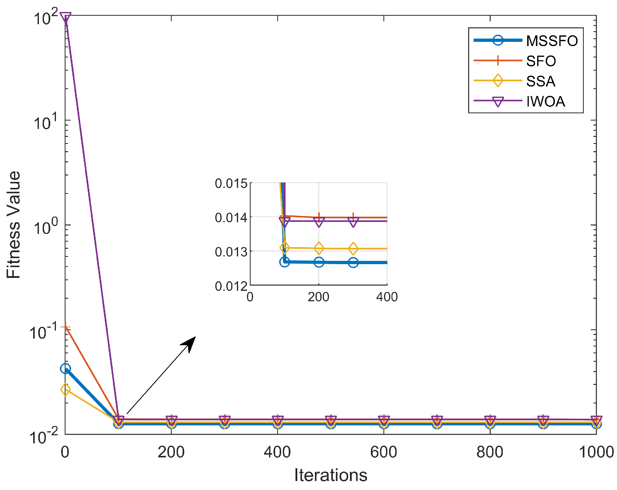
The optimization results of the CSD problem for the MSSFO are compared with the GA, PSO, weighted chimp optimization (WCHO), the SFO, the SSA, and the IWOA, and the results are presented in

Table 13. Comparison of the MSSFO results with other algorithms for tension/compression spring design problem.

Algorithm	d	D	P	Mean Fitness
GA [86]	0.0524	0.3521	11.5980	0.032
PSO [86]	0.0500	0.3104	14.998	0.0131
WCHO [86]	0.0508	0.3142	14.4314	0.0134
MSSFO	0.0556	0.4594	7.5262	0.0130
SFO	0.0572	0.5124	6.7111	0.0135
SSA	0.0530	0.3988	11.2036	2.2940
IWOA	0.0584	0.5483	5.8836	0.0137

. The GA, PSO, and WCHO results are taken from the literature [86], and the rest of the results have been generated. Each algorithm is independently run 30 times, and the maximum number of iterations is set to 1000. These settings are consistent with the literature [86]. From Table 13, it is evident that the performance of the MSSFO is better than all other nature-inspired optimization algorithms, as it provides the best solutions among all. Further analysis using the convergence curve of the median values is presented in Figure 6.

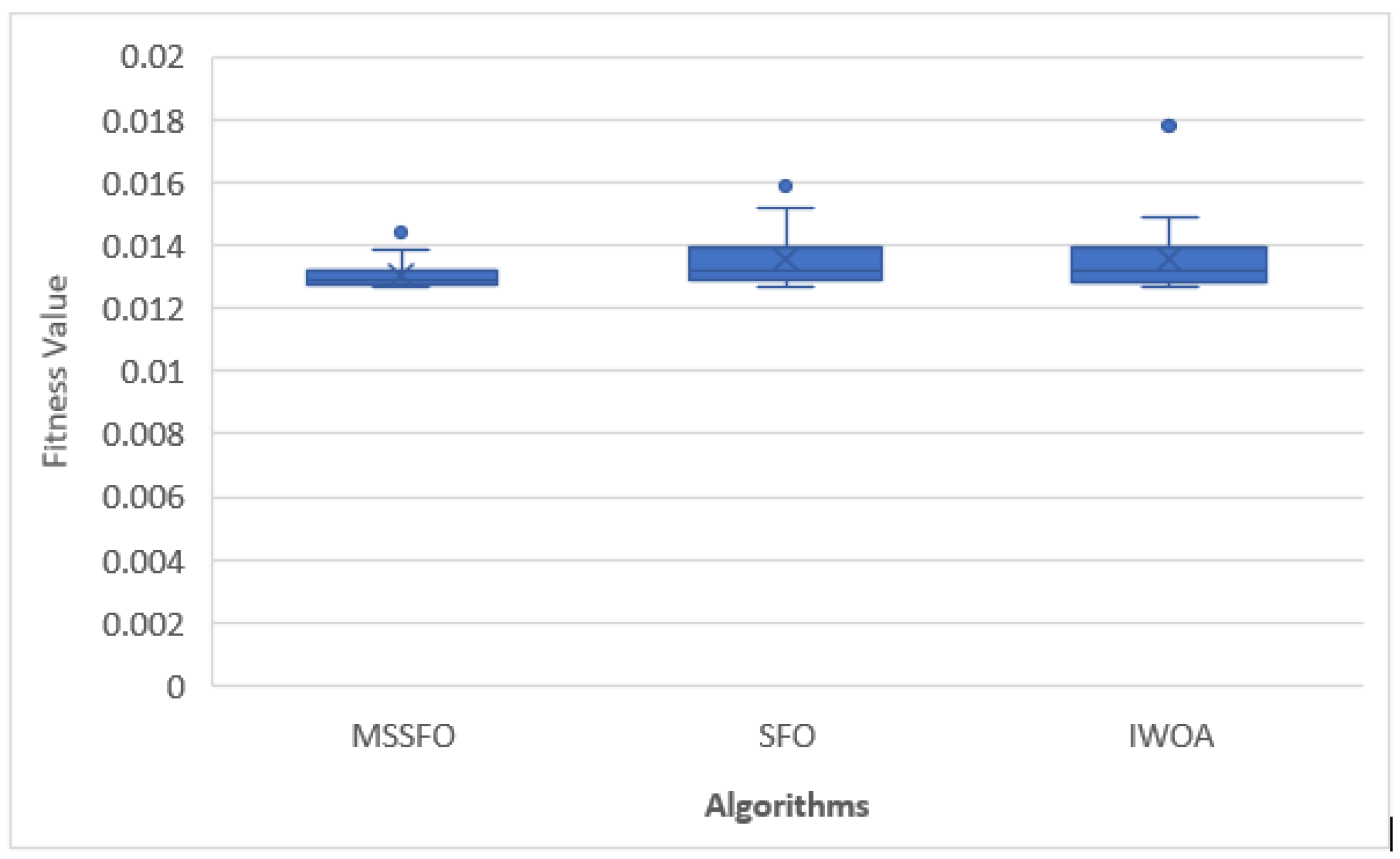
It can be observed from Table 13 and Figure 6 and Figure 7 that the MSSFO shows better performance compared with all the other algorithms applied in the CSD problem and improves the quality of solutions for the selected problem.

4.7. Performance Evaluation on Mobile Robot Path Planning Problem

Path planning is a fundamental aspect of mobile robot technology, with the primary goal of determining a safe and optimal route from a given starting point to the target destination [87]. The objective here is to minimize the path length in the presence of various obstacles. Given a solution that represents a path consisting of a series of nodes in a graph, the fitness value can be computed as the total sum of distances between consecutive nodes, from the start node to the destination node, presented by the following equation:

$$\mathrm{Fitness}\left(F\right)=\sum _{i=1}^{N-1}d(P_i,P_{i+1})$$

The Euclidean distance between two consecutive points $P_i(x_i,y_i)$ and $P_{i+1}(x_{i+1},y_{i+1})$ is given by

$$d(P_i,P_{i+1})=\sqrt{{(x_{i+1}-x_i)}^2+{(y_{i+1}-y_i)}^2}.$$

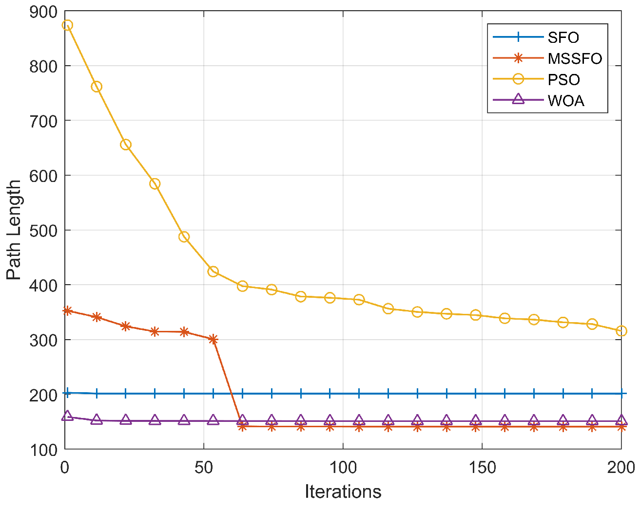
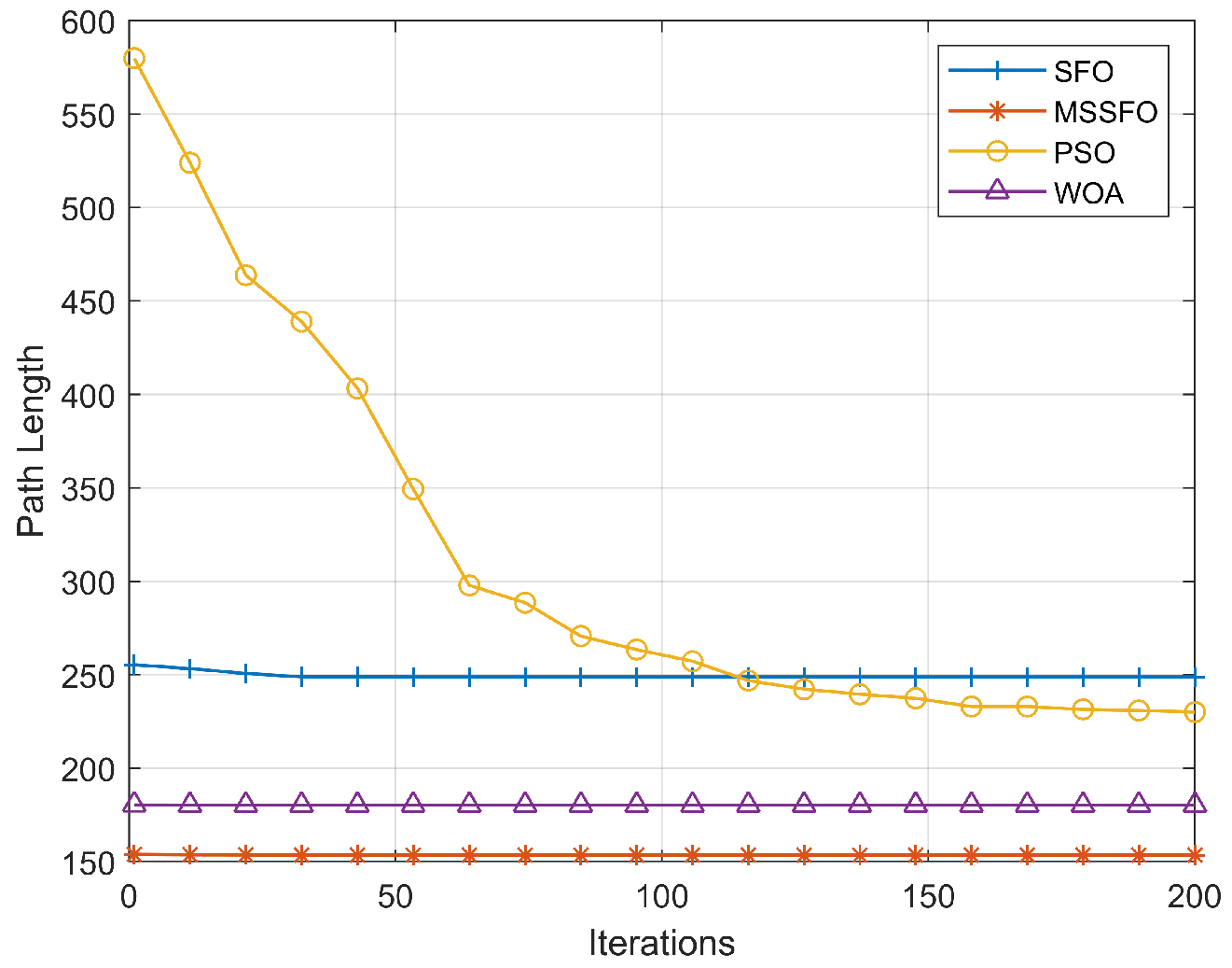
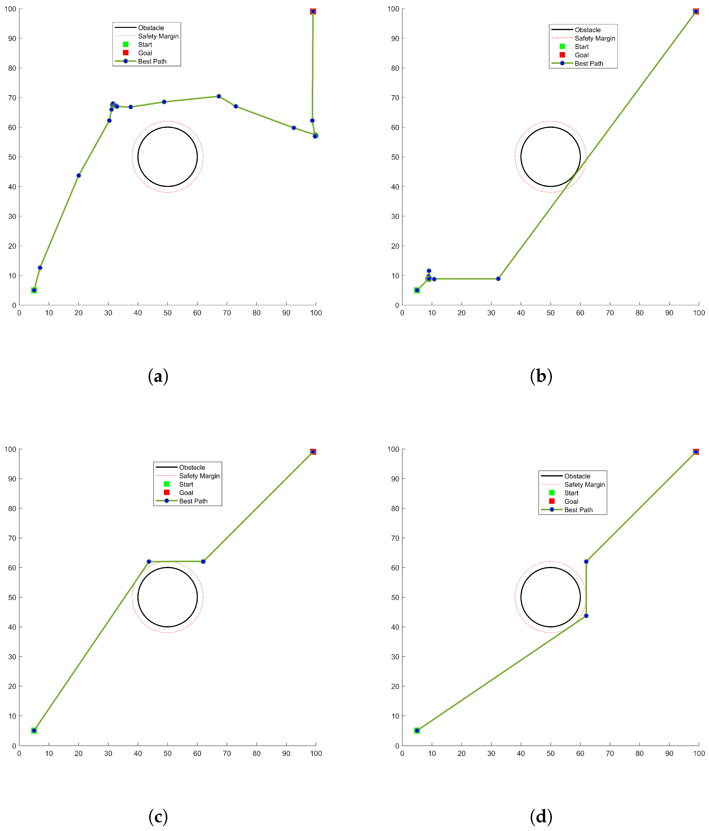
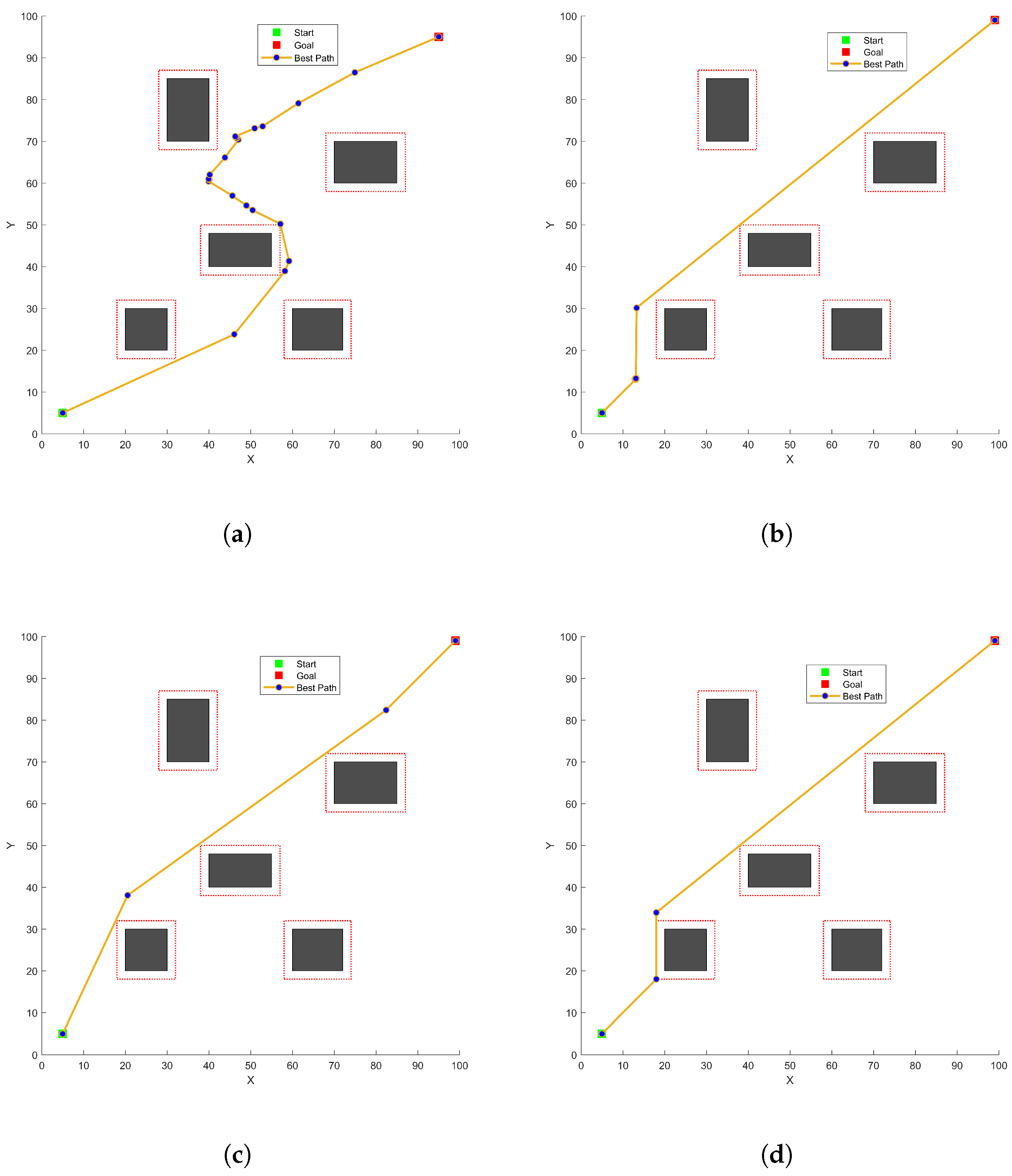
Two scenarios are considered for this problem, where scenario one uses one circular obstacle and scenario two uses multiple regularly shaped obstacles in a 100 × 100 2D environment. Multiple path points are setup for the simulation starting from (5, 5) and ending at (99, 99). The start and end points are determined and kept constant before running the simulation. The path points are randomly generated within the boundary of the environment. The initial population is set to 20, and the number of runs is 30, whereas the number of iterations for each run is set to 200. For a fair comparison, these settings are kept consistent for all the algorithms. Other algorithms used for comparison are the PSO, the SFO, and the WOA. The optimal results for the two scenarios (after 30 independent runs) are reported in

Table 14. Comparison of the MSSFO with other algorithms on the mobile robot path planning problem using one circular obstacle.

Algorithm	Best Path Length	Average Path Length	Std. Dev.
MSSFO	139.5648	176.0337	39.8151
WOA	139.5343	1381.7761	6642.2654
PSO	183.7413	371.2224	118.4736
SFO	155.5843	1955.6175	6763.5753

and

Table 15. Comparison of the MSSFO with other algorithms on the mobile robot path planning problem using multiple obstacles.

Algorithm	Best Path Length	Average Path Length	Std. Dev.
MSSFO	136.1217	179.8756	74.6789
WOA	138.2446	933,488.3621	1,337,344.7480
PSO	164.2967	233,660.4280	430,180.6187
SFO	140.1128	733,551.9436	1,014,830.7897

. Convergence behavior for all the algorithms utilized in scenario 1 and scenario 2 are visualized in Figure 8 and Figure 9, respectively. Optimal paths selected by various algorithms using two scenarios are presented in Figure 10 and Figure 11.

It is observed from Table 14 that the MSSFO and WOA perform similarly in finding a minimum (best) distance; however, there is a clear difference in average performance, which confirms the robustness of the proposed MSSFO. As a result, the MSSFO exhibits the best average path length with a minimal deviation. This is further verified when the MSSFO is applied to the second scenario (with multiple obstacles), where the MSSFO performs better than all the other algorithms, with the minimum best path length, the minimum average path length, and a minimal deviation from the results.

The superiority of the MSSFO can be further verified by the convergence curve presented in Figure 8 and Figure 9. For the single-obstacle scenario, it can be seen that the WOA and the MSSFO are competitive, whereas the MSSFO outperforms all the other algorithms when the multiple-obstacle environment is created. This verifies the effectiveness and efficiency of the MSSFO in solving the mobile robot path planning problem, which can be further explored in complex environments with multiple irregularly shaped obstacles, more path points, or multiple robots.

5. Discussion

The sailfish optimizer (SFO) has gained considerable attention since its introduction, with numerous improvements and applications proposed in the literature. In this study, a new enhanced variant of the SFO, referred to as the Multi-Strategy Sailfish Optimizer (MSSFO), has been developed by integrating multiple strategies, including an improved search mechanism, a non-linear attack power (AP) parameter, a modified hunting process, and a novel dynamic sardine population technique. The experimental results have been systematically presented in the previous section.

Parameter sensitivity analysis is a crucial step in laying down the basis for further experimentation. Three internal parameters, $\alpha$, $\beta$, and a were experimentally evaluated with different combinations to find suitable values for further experimentation. The mean results and a Friedman mean rank were used to select the best combinations, and the final values of parameter a, $\alpha$, and $\beta$ turned out to be 2, 0.01, and 0.2, respectively.

Next, the impact of each modification individually and in combination was studied and applied to the original SFO. Twelve minimization problems from the CEC 2022 test suite were utilized for the experimentation purposes. F1 is the only unimodal problem, and interestingly, none of the techniques individually impacted the solution significantly. However, when the modified search strategy was combined with a dynamic sardine population (MSFO-AD), the result for F1 was significantly improved. Furthermore, when all the techniques were combined together, the algorithm successfully found the optimal solution, as the error value reached zero for F1. In the multimodal problems (F2 to F5), the dynamic sardine population (MSFO-D) strategy improved the original SFO and achieved better performance than the SFO in all the problems. The hybrid functions (F6 to F8) seemed more challenging, and a very slight improvement was observed with the MSFO-A, MSFO-B, and MSFO-D strategies in all the three problems. The last category is that of the composite functions (F9 to F12), and the MSFO-D strategy showed improvement and achieved the best rank for these functions.

It is important to note that modifying the search strategy (MSFO-A) alone provided a slight improvement, less than 2% overall. However, when the MSFO-A was combined with the MSFO-C or MSFO-D strategy, the performance improved significantly. Similarly, the modified hunting technique, MSFO-C, alone has limited or no impact, but when integrated with the modified search strategy (MSFO-AC), it yielded notable performance, gaining an overall 33% improvement. The two most effective techniques, MSFO-A and MSFO-D, combined together as the MSFO-AD, achieved the best results, providing an overall improvement of 76%, obtaining a higher rank than any other modification. The final version, the MSSFO, combining all the proposed strategies, showed 80% improvement over the original SFO, making it the best choice among all the tested variants. To further analyze the significance of the MSSFO, the Wilcoxon signed-rank test was performed at a 95% significance level, which again resulted in a p-value lower than 0.05. This validates that the MSSFO significantly improves the SFO and can be further evaluated with other optimization algorithms.

After validation, the performance of the MSSFO was compared with the other well-known optimization algorithms, including the SFO, two other variants of the SFO, the SCA, the ISCA, the WOA, and the IWOA, as discussed in Section 4.4. The MSSFO is evidently the best optimizer for 10-dimensional problems, except for F10, where the MSSFO achieved a second rank. However, it ranked at the top when the average was calculated. For 20-dimensional problems, the MSSFO was competitive with respect to the SCA and the ISCA and significantly better than all other algorithms and remained on top in the average ranking. The convergence curves were also presented to show the fast convergence capabilities of the MSSFO.

A statistical analysis is essential to identifying the significant differences among the optimization methods. Since the non-parametric tests do not rely on strict data assumptions [88], they are appropriate for comparing the stochastic optimizers. In this study, the Friedman test was used to analyze rankings for both the 10- and 20-dimensional problems. The results confirmed the statistical significance of the MSSFO’s superior performance. A pairwise Wilcoxon signed-rank test was also conducted to compare the MSSFO against each algorithm individually, and again, the MSSFO showed statistically significant improvements with p-values below the 0.05 threshold.

Finally, the MSSFO was applied to two real-world problems. The first application was to minimize the spring weight for the compression spring design (CSD) problem. The results showed that the MSSFO is robust when applied to the CSD problem. It is also evident from the convergence graph that the MSSFO has the capability of performing better exploitation of the search space and that it converges quickly towards the optimal/near-optimal solution. Furthermore, the box plot for 30 optimal values of the CSD problem validates the efficacy and accuracy of the MSSFO in finding optimal solutions with robustness.

The second real-world problem evaluated in this study was the mobile robot path planning problem. The objective is to minimize the path length of a mobile robot while avoiding the obstacles encountered during the journey. Two environments were set up, the first with one obstacle and the second one with five multi-shaped obstacles. In the first scenario, although the MSSFO was competitive with respect to the WOA in finding the minimum path length, the average path length was significantly better than that of the WOA. This confirms the robustness of the proposed algorithm. In the second scenario, where five obstacles were placed, the MSSFO was the best optimizer with the lowest average path length and minimum deviation. The convergence curves of both the scenarios verified the effectiveness of the MSSFO in solving the robot path planning problem.

Overall, the performance of the MSSFO was significantly better than the comparison algorithms in solving the CEC 2022 SO-BO problems and the two real-world problems considered in this study, hence confirming the significance of the MSSFO as a potential candidate for solving real-world optimization problems with efficacy and robustness.

Future Research Directions

The superiority of the MSSFO raises several important open research directions that warrant further investigation. One key question is its ability to solve more complex real-world problems, like the robot path planning with various irregularly shaped obstacles, multi-robot path planning, and feature selection in machine learning, among others. Another open challenge is the scalability of the MSSFO to high-dimensional, real-time, or industrial-scale optimization problems, raising the question of whether hybridized or parallel implementations could enhance its efficiency. The modifications proposed in this study open several avenues for further investigation. The observed standalone effects of the proposed strategies indicate that the modified hunting mechanism merits further independent investigation to achieve maximum benefit and improve solution quality. Furthermore, multi-objective and many-objective variants of the MSSFO can also be developed and tested on real-world problems. The motivation for the development of such algorithms is the demand of recent complex problems in the areas of engineering and science. These open research directions provide a basis for advancing both theoretical development and real-world applicability in future research.

6. Conclusions

In this study, an improved variant of the sailfish optimizer (SFO), named the Multi-Strategy Sailfish Optimizer (MSSFO), is developed by integrating several improvement strategies, including an improved search strategy, a non-linear AP parameter, a modified hunting mechanism, and dynamic sardine population. The proposed modifications were designed to strengthen the algorithm’s search capability, balance exploration and exploitation, and improve the overall solution accuracy. Based on the experimental evaluation, the MSSFO demonstrated strong optimization performance and reliable convergence behavior. The findings confirm that the MSSFO is a robust and effective optimization method suitable for a wide range of benchmark and real-world problems. The integrated improvements enable it to achieve competitive results across diverse problem types. Overall, the MSSFO represents a significant improved variant of the original SFO and provides a solid foundation for future extensions and applications.

References

1. Laporte, G. The traveling salesman problem: An overview of exact and approximate algorithms. Eur. J. Oper. Res. 1992, 59, 231–247. [Google Scholar] [CrossRef]
2. Zhou, T.; Wei, W. Mobile robot path planning based on an improved ACO algorithm and path optimization. Multimed. Tools Appl. 2025, 84, 10899–10922. [Google Scholar] [CrossRef]
3. Larabi-Marie-Sainte, S.; Bin Alamir, M.; Alameer, A. Arabic Text Clustering Using Self-Organizing Maps and Grey Wolf Optimization. Appl. Sci. 2023, 13, 10168. [Google Scholar] [CrossRef]
4. Kumar, M.; Suman, S. Scheduling in IaaS Cloud Computing Environment using Sailfish Optimization Algorithm. Trends Sci. 2022, 19, 4204. [Google Scholar] [CrossRef]
5. Rajamoorthy, R.; Arunachalam, G.; Kasinathan, P.; Devendiran, R.; Ahmadi, P.; Pandiyan, S.; Muthusamy, S.; Panchal, H.; Kazem, H.A.; Sharma, P. A novel intelligent transport system charging scheduling for electric vehicles using Grey Wolf Optimizer and Sail Fish Optimization algorithms. Energy Sources Part A Recover. Util. Environ. Eff. 2022, 44, 3555–3575. [Google Scholar] [CrossRef]
6. Zhang, Y.; Mo, Y. Dynamic optimization of chemical processes based on modified sailfish optimizer combined with an equal division method. Processes 2021, 9, 1806. [Google Scholar] [CrossRef]
7. Ren, X.; Ma, L. Main Steam Temperature Load Tracking Control Based on Improved Sailfish Optimization. In Proceedings of the Energy Proceedings (International Conference on Applied Energy—ICAE 2020), Bangkok, Thailand, 1–10 December 2020. [Google Scholar] [CrossRef]
8. Li, L.L.; Shen, Q.; Tseng, M.L.; Luo, S. Power system hybrid dynamic economic emission dispatch with wind energy based on improved sailfish algorithm. J. Clean. Prod. 2021, 316, 128318. [Google Scholar] [CrossRef]
9. Antwi, R.; Gadze, J.D.; Tchao, E.T.; Sikora, A.; Obour Agyekum, K.O.B.; Nunoo-Mensah, H.; Agbemenu, A.S.; Agyemang, J.O.; Welte, D.; Ahmed, A.R.; et al. Optimising peer-to-peer topology for blockchain-based industrial internet of things networks using particle swarm optimisation. Clust. Comput. 2025, 28, 204. [Google Scholar] [CrossRef]
10. Tounsi, M.; Ali, H.; Azar, A.T.; Al-Khayyat, A.; Ibraheem, I.K. Comprehensive Learning Salp Swarm Algorithm with Ensemble Deep Learning-based ECG Signal Classification on Internet of Things Environment. Eng. Technol. Appl. Sci. Res. 2025, 15, 19492–19500. [Google Scholar] [CrossRef]
11. Wu, M. Application of particle swarm optimisation algorithm incorporating frog-leaping algorithm in optimal scheduling for production management in manufacturing plant. Int. J. Interact. Des. Manuf. (IJIDeM) 2025, 19, 1721–1735. [Google Scholar] [CrossRef]
12. Kumar, L.; Goyal, A.; Pathak, V.K.; Bhowmik, A. A state-of-the-art review of soft computing-based monitoring and control in the machining of hard alloys. Discov. Appl. Sci. 2025, 7, 681. [Google Scholar] [CrossRef]
13. Zambou, M.C.Z.; Kammogne, A.S.T.; Siewe, M.S.; Azar, A.T.; Ahmed, S.; Hameed, I.A. Optimized Nonlinear PID Control for Maximum Power Point Tracking in PV Systems Using Particle Swarm Optimization. Math. Comput. Appl. 2024, 29, 88. [Google Scholar] [CrossRef]
14. Mahmood, S.; Bawany, N.Z.; Tanweer, M.R. A comprehensive survey of Whale Optimization Algorithm: Modifications and classification. Indones. J. Electr. Eng. Comput. Sci. 2023, 29, 899–910. [Google Scholar] [CrossRef]
15. Yang, X.S. Nature-inspired optimization algorithms: Challenges and open problems. J. Comput. Sci. 2020, 46, 101104. [Google Scholar] [CrossRef]
16. Moshtaghi, H.R.; Eshlaghy, A.T.; Motadel, M.R. A Comprehensive Review on Meta-Heuristic Algorithms and their Classification with Novel Approach. J. Appl. Res. Ind. Eng. 2021, 8, 63–89. [Google Scholar] [CrossRef]
17. Holland, J.H. Genetic Algorithms. Sci. Am. 1992, 267, 66–72. [Google Scholar] [CrossRef]
18. Beyer, H.G. Toward a Theory of Evolution Strategies: The (μ, λ)-Theory. Evol. Comput. 1994, 2, 381–407. [Google Scholar] [CrossRef]
19. Storn, R.; Price, K. Differential evolution–a simple and efficient heuristic for global optimization over continuous spaces. J. Glob. Optim. 1997, 11, 341–359. [Google Scholar] [CrossRef]
20. Dorigo, M.; Maniezzo, V.; Colorni, A. Ant system: Optimization by a colony of cooperating agents. IEEE Trans. Syst. Man, Cybern. Part B Cybern. 1996, 26, 29–41. [Google Scholar] [CrossRef]
21. Kennedy, J.; Eberhart, R. Particle swarm optimization. In Proceedings of the ICNN’95—International Conference on Neural Networks, Perth, WA, Australia, 27 November 1995–1 December 1995; Volume 26, pp. 1942–1948. [Google Scholar] [CrossRef]
22. Yang, X.S.; Gandomi, A.H. Bat algorithm: A novel approach for global engineering optimization. Eng. Comput. 2012, 29, 464–483. [Google Scholar] [CrossRef]
23. Mirjalili, S. SCA: A sine cosine algorithm for solving optimization problems. Knowl.-Based Syst. 2016, 96, 120–133. [Google Scholar] [CrossRef]
24. Mirjalili, S.; Lewis, A. Advances in Engineering Software The Whale Optimization Algorithm. Adv. Eng. Softw. 2016, 95, 51–67. [Google Scholar] [CrossRef]
25. Mirjalili, S.; Mirjalili, S.M.; Lewis, A. Grey Wolf Optimizer. Adv. Eng. Softw. 2014, 69, 46–61. [Google Scholar] [CrossRef]
26. Braik, M.; Hammouri, A.; Atwan, J.; Al-Betar, M.A.; Awadallah, M.A. White Shark Optimizer: A novel bio-inspired meta-heuristic algorithm for global optimization problems. Knowl.-Based Syst. 2022, 243, 108457. [Google Scholar] [CrossRef]
27. Rao, R.V.; Savsani, V.J.; Vakharia, D.P. Teaching-learning-based optimization: A novel method for constrained mechanical design optimization problems. CAD Comput. Aided Des. 2011, 43, 303–315. [Google Scholar] [CrossRef]
28. Shadravan, S.; Naji, H.R.; Bardsiri, V.K. The Sailfish Optimizer: A novel nature-inspired metaheuristic algorithm for solving constrained engineering optimization problems. Eng. Appl. Artif. Intell. 2019, 80, 20–34. [Google Scholar] [CrossRef]
29. Abualigah, L.; Diabat, A.; Mirjalili, S.; Elaziz, M.A.; Gandomi, A.H. The Arithmetic Optimization Algorithm. Comput. Methods Appl. Mech. Eng. 2021, 376, 113609. [Google Scholar] [CrossRef]
30. Khishe, M.; Mosavi, M.R. Chimp optimization algorithm. Expert Syst. Appl. 2020, 149, 113338. [Google Scholar] [CrossRef]
31. Li, H.; Liu, X.; Huang, Z.; Zeng, C.; Zou, P.; Chu, Z.; Yi, J. Newly Emerging Nature-Inspired Optimization-Algorithm Review, Unified Framework, Evaluation, and Behavioural Parameter Optimization. IEEE Access 2020, 8, 72620–72649. [Google Scholar] [CrossRef]
32. Siddique, N.; Adeli, H. Nature Inspired Computing: An Overview and Some Future Directions. Cogn. Comput. 2015, 7, 706–714. [Google Scholar] [CrossRef]
33. Tzanetos, A.; Dounias, G. Nature inspired optimization algorithms or simply variations of metaheuristics? Artif. Intell. Rev. 2021, 54, 1841–1862. [Google Scholar] [CrossRef]
34. Suid, M.H.; Ahmad, M.A.; Ismail, M.R.T.R.; Ghazali, M.R.; Irawan, A.; Tumari, M.Z. An Improved Sine Cosine Algorithm for Solving Optimization Problems. In Proceedings of the 2018 IEEE Symposium on Computer Applications & Industrial Electronics (SPC), Melaka, Malaysia, 14–15 December 2018. [Google Scholar] [CrossRef]
35. Tanweer, M.R.; Auditya, R.; Suresh, S.; Sundararajan, N.; Srikanth, N. Directionally Driven Self-Regulating Particle Swarm Optimization algorithm. Swarm Evol. Comput. 2016, 28, 98–116. [Google Scholar] [CrossRef]
36. Tudose, A.M.; Picioroaga, I.I.; Sidea, D.O.; Bulac, C. Solving single-and multi-objective optimal reactive power dispatch problems using an improved salp swarm algorithm. Energies 2021, 14, 1222. [Google Scholar] [CrossRef]
37. Taheri, A.; RahimiZadeh, K.; Rao, R.V. An efficient Balanced Teaching-Learning-Based optimization algorithm with Individual restarting strategy for solving global optimization problems. Inf. Sci. 2021, 576, 68–104. [Google Scholar] [CrossRef]
38. Pandey, A.C.; Tikkiwal, V.A. Stance detection using improved whale optimization algorithm. Complex Intell. Syst. 2021, 7, 1649–1672. [Google Scholar] [CrossRef]
39. Wolpert, D.H.; Macready, W.G. No free lunch theorems for optimization. IEEE Trans. Evol. Comput. 1997, 1, 67–82. [Google Scholar] [CrossRef]
40. Issam, E.H.; Lajjam, A.; Merouani, M.E.; Tabaa, Y. A modified sailfish optimizer to solve dynamic berth allocation problem in conventional container terminal. Int. J. Ind. Eng. Comput. 2019, 10, 491–504. [Google Scholar] [CrossRef]
41. Ghosh, K.K.; Ahmed, S.; Singh, P.K.; Geem, Z.W.; Sarkar, R. Improved binary sailfish optimizer based on adaptive B-Hill climbing for feature selection. IEEE Access 2020, 8, 83548–83560. [Google Scholar] [CrossRef]
42. Zhang, Y.; Mo, Y. Chaotic adaptive sailfish optimizer with genetic characteristics for global optimization. J. Supercomput. 2022, 78, 10950–10996. [Google Scholar] [CrossRef]
43. Mohammadi, R.; Akleylek, S.; Ghaffari, A. SDN-IoT: SDN-based efficient clustering scheme for IoT using improved Sailfish optimization algorithm. PeerJ Comput. Sci. 2023, 9, e1424. [Google Scholar] [CrossRef] [PubMed]
44. Hongfei, L.; Guohui, Z.; Huang, B.; Chi, M.A.; Gong, C.; Jinbin, Z. Optimal Control Virtual Inertia of Optical Storage Microgrid Based on Improved Sailfish Algorithm. Wuhan Univ. J. Nat. Sci. 2022, 27, 218–230. [Google Scholar] [CrossRef]
45. Shajin, F.H.; Devi, B.A.; Prakash, N.B.; Sreekanth, G.R.; Rajesh, P. Sailfish optimizer with Levy flight, chaotic and opposition-based multi-level thresholding for medical image segmentation. Soft Comput. 2023, 27, 12457–12482. [Google Scholar] [CrossRef]
46. Cao, L.; Yue, Y.; Chen, Y.; Chen, C.; Chen, B. Sailfish optimization algorithm integrated with the osprey optimization algorithm and cauchy mutation and its engineering applications. Symmetry 2025, 17, 938. [Google Scholar] [CrossRef]
47. Amin, S.A.; Alqudah, M.K.S.; Almutairi, S.A.; Almajed, R.; Al Nasar, M.R.; Alkhazaleh, H.A. Optimal extreme learning machine for diagnosing brain tumor based on modified sailfish optimizer. Heliyon 2024, 10, e34050. [Google Scholar] [CrossRef]
48. Babu, J.S.; Niranjana, G.; Ramana, K. Adaptive sail fish optimizer based optimized region selection for robust video steganography. Int. J. Inf. Technol. 2025, 17, 2417–2427. [Google Scholar] [CrossRef]
49. Sedak, M.; Rosić Vitas, M.; Rosić, B. Multi-objective hybrid sailfish optimization algorithm for planetary gearbox and mechanical engineering design optimization problems. Comput. Model. Eng. Sci. 2025, 142, 2111–2145. [Google Scholar] [CrossRef]
50. Azzam, S.M.; Emam, O.; Abolaban, A.S. An improved Differential evolution with Sailfish optimizer (DESFO) for handling feature selection problem. Sci. Rep. 2024, 14, 13517. [Google Scholar] [CrossRef]
51. Li, M.; Li, Y.; Chen, Y.; Xu, Y. Batch recommendation of experts to questions in community-based question-answering with a sailfish optimizer. Expert Syst. Appl. 2021, 169, 114484. [Google Scholar] [CrossRef]
52. Togacar, M.; Ergen, B. Classification of cloud images by using super resolution, semantic segmentation approaches and binary sailfish optimization method with deep learning model. Comput. Electron. Agric. 2022, 193, 106724. [Google Scholar] [CrossRef]
53. Naji, H.R.; Shadravan, S.; Jafarabadi, H.M.; Momeni, H. Accelerating sailfish optimization applied to unconstrained optimization problems on graphical processing unit. Eng. Sci. Technol. Int. J. 2022, 32, 101077. [Google Scholar] [CrossRef]
54. Shadravan, S.; Naji, H.R.; Khatibi, V. A Distributed Sailfish Optimizer Based on Multi-Agent Systems for Solving Non-Convex and Scalable Optimization Problems Implemented on GPU. Technol. J. Artif. Intell. Data Min. 2021, 9, 59–71. [Google Scholar] [CrossRef]
55. Geetha, P.; Nanda, S.J.; Yadav, R.P. A parallel chaotic sailfish optimization algorithm for estimation of DOA in wireless sensor array. Phys. Commun. 2022, 51, 101536. [Google Scholar] [CrossRef]
56. Hammouti, I.E.; Lajjam, A.; Merouani, M.E. Comparison of planning models for dynamic berth allocation problem using a sailfish-based algorithm. Procedia Comput. Sci. 2020, 176, 3112–3120. [Google Scholar] [CrossRef]
57. Sankar, S.; Ramasubbareddy, S.; Chen, F.; Gandomi, A.H. Energy-Efficient Cluster-Based Routing Protocol in Internet of Things Using Swarm Intelligence. In Proceedings of the 2020 IEEE Symposium Series on Computational Intelligence (SSCI), Canberra, ACT, Australia, 1–4 December 2020; pp. 219–224. [Google Scholar] [CrossRef]
58. Amutha, R.; Sivasankari, G.G.; Venugopal, K.R. Node clustering and data aggregation in wireless sensor network using sailfish optimization. Multimed. Tools Appl. 2023, 82, 44107–44122. [Google Scholar] [CrossRef]
59. Mehta, D.; Saxena, S. MCH-EOR: Multi-objective Cluster Head Based Energy-aware Optimized Routing algorithm in Wireless Sensor Networks. Sustain. Comput. Inform. Syst. 2020, 28, 100406. [Google Scholar] [CrossRef]
60. Kumar, M.; Ali, J. Taylor Sailfish Optimizer-Based Deep Stacked Auto Encoder for Blackhole Attack Detection in Wireless Sensor Network. J. Web Eng. 2022, 21, 911–940. [Google Scholar] [CrossRef]
61. Kumar, B.S.; Santhi, S.G.; Narayana, S. Sailfish optimizer algorithm (SFO) for optimized clustering in wireless sensor network (WSN). J. Eng. Des. Technol. 2021, 20, 1449–1467. [Google Scholar] [CrossRef]
62. Rajoriya, M.K.; Gupta, C.P. Sailfish optimization-based controller selection (SFO-CS) for energy-aware multi-hop routing in software defined wireless sensor network (SDWSN). Int. J. Inf. Technol. 2023, 15, 3935–3948. [Google Scholar] [CrossRef]
63. Samal, P.; Roshan, R. Optimal STATCOM allocation and sizing using the sailfish optimizer algorithm. In Proceedings of the 2020 IEEE 7th Uttar Pradesh Section International Conference on Electrical, Electronics and Computer Engineering (UPCON), Prayagraj, India, 27–29 November 2020; pp. 1–6. [Google Scholar] [CrossRef]
64. Duhayyim, M.A.; Malibari, A.A.; Dhahbi, S.; Nour, M.K.; Al-Turaiki, I.; Obayya, M.; Mohamed, A. Sailfish Optimization with Deep Learning Based Oral Cancer Classification Model. Comput. Syst. Sci. Eng. 2023, 45, 753–767. [Google Scholar] [CrossRef]
65. Hamza, M.A.; Hassine, S.B.H.; Abunadi, I.; Al-Wesabi, F.N.; Alsolai, H.; Hilal, A.M.; Yaseen, I.; Motwakel, A. Feature Selection with Optimal Stacked Sparse Autoencoder for Data Mining. Comput. Mater. Contin. 2022, 72, 2581–2596. [Google Scholar] [CrossRef]
66. Selvapandian, A.; N. Prabhu, S.; Sivakumar, P.; J. Rao, D.B. Lung cancer detection and severity level classification using sine cosine sail fish optimization based generative adversarial network with CT images. Comput. J. 2022, 65, 1611–1630. [Google Scholar] [CrossRef]
67. Khan, N.M.; Khan, U.A.; Zafar, M.H. Maximum power point tracking of PV system under uniform irradiance and partial shading conditions using machine learning algorithm trained by sailfish optimizer. In Proceedings of the 2021 4th International Conference on Energy Conservation and Efficiency (ICECE), Lahore, Pakistan, 16–17 March 2021; pp. 1–6. [Google Scholar] [CrossRef]
68. Alqahtani, M.M.; Dutta, A.K.; Almotairi, S.; Ilayaraja, M.; Albraikan, A.A.; Al-Wesabi, F.N.; Duhayyim, M.A. Sailfish Optimizer with EfficientNet Model for Apple Leaf Disease Detection. Comput. Mater. Contin. 2023, 74, 217–233. [Google Scholar] [CrossRef]
69. Nagapavithra, S.; Umamaheswari, S. Detection and classification of sugarcane billet damage using Aquila Sailfish Optimizer based deep learning. Artif. Intell. Rev. 2023, 56, 2183–2206. [Google Scholar] [CrossRef]
70. Gutte, V.S.; Parasar, D. Sailfish invasive weed optimization algorithm for multiple image sharing in cloud computing. Int. J. Intell. Syst. 2022, 37, 4190–4213. [Google Scholar] [CrossRef]
71. Kalpana, P. Chronological sailfish optimizer for preserving privacy in cloud based on khatri-rao product. Comput. J. 2021, 66, 101–113. [Google Scholar] [CrossRef]
72. Nassef, M.G.A.; Hussein, T.M.; Mokhiamar, O. An adaptive variational mode decomposition based on sailfish optimization algorithm and Gini index for fault identification in rolling bearings. Measurement 2021, 173, 108514. [Google Scholar] [CrossRef]
73. Rai, A.; Das, D.K. The development of a fuzzy tilt integral derivative controller based on the sailfish optimizer to solve load frequency control in a microgrid, incorporating energy storage systems. J. Energy Storage 2022, 48, 103887. [Google Scholar] [CrossRef]
74. Cheng, X.; Li, J.; Zheng, C.; Zhang, J.; Zhao, M. An improved PSO-GWO algorithm with chaos and adaptive inertial weight for robot path planning. Front. Neurorobotics 2021, 15, 770361. [Google Scholar] [CrossRef] [PubMed]
75. Ab Wahab, M.N.; Nazir, A.; Khalil, A.; Ho, W.J.; Akbar, M.F.; Noor, M.H.M.; Mohamed, A.S.A. Improved genetic algorithm for mobile robot path planning in static environments. Expert Syst. Appl. 2024, 249, 123762. [Google Scholar] [CrossRef]
76. Cui, J.; Wu, L.; Huang, X.; Xu, D.; Liu, C.; Xiao, W. Multi-strategy adaptable ant colony optimization algorithm and its application in robot path planning. Knowledge-Based Syst. 2024, 288, 111459. [Google Scholar] [CrossRef]
77. Sun, J.; Feng, B.; Xu, W. Particle swarm optimization with particles having quantum behavior. In Proceedings of the 2004 Congress on Evolutionary Computation (IEEE Cat. No. 04TH8753), Portland, OR, USA, 19–23 June 2004; IEEE: Piscataway, NJ, USA, 2004; Volume 1, pp. 325–331. [Google Scholar] [CrossRef]
78. Sun, J.; Xu, W.; Feng, B. A global search strategy of quantum-behaved particle swarm optimization. In Proceedings of the IEEE Conference on Cybernetics and Intelligent Systems, Singapore, 1–3 December 2004; IEEE: Piscataway, NJ, USA, 2004; Volume 1, pp. 111–116. [Google Scholar] [CrossRef]
79. Kononova, A.V.; Corne, D.W.; De Wilde, P.; Shneer, V.; Caraffini, F. Structural bias in population-based algorithms. Inf. Sci. 2015, 298, 468–490. [Google Scholar] [CrossRef]
80. Long, W.; Wu, T.; Liang, X.; Xu, S. Solving high-dimensional global optimization problems using an improved sine cosine algorithm. Expert Syst. Appl. 2019, 123, 108–126. [Google Scholar] [CrossRef]
81. Kumar, A.; Price, K.; Mohamed, A.W.; Hadi, A.A.; Suganthan, P.N. Problem definitions and evaluation criteria for the CEC 2022 special session and competition on Single Objective Bound Constrained Numerical Optimization. Tech. Rep. 2021. [Google Scholar] [CrossRef]
82. Derrac, J.; García, S.; Molina, D.; Herrera, F. A practical tutorial on the use of nonparametric statistical tests as a methodology for comparing evolutionary and swarm intelligence algorithms. Swarm Evol. Comput. 2011, 1, 3–18. [Google Scholar] [CrossRef]
83. Sheskin, D.J. Handbook of Parametric and Nonparametric Statistical Procedures, 3rd ed.; CRC Press: Boca Raton, FL, USA, 2003. [Google Scholar] [CrossRef]
84. Davenport, J.M. Approximations of the critical region of the Friedman statistic. Commun. Stat. Theory Methods 1980, 9, 571–595. [Google Scholar] [CrossRef]
85. García, S.; Fernández, A.; Luengo, J.; Herrera, F. A study of statistical techniques and performance measures for genetics-based machine learning: Accuracy and interpretability. Soft Comput. 2009, 13, 959–977. [Google Scholar] [CrossRef]
86. Zhang, Q.; Du, S.; Zhang, Y.; Wu, H.; Duan, K.; Lin, Y. A Novel Chimp Optimization Algorithm with Refraction Learning and Its Engineering Applications. Algorithms 2022, 15, 189. [Google Scholar] [CrossRef]
87. Massoud, M.M.; Abdellatif, A.; Atia, M.R. Different path planning techniques for an indoor omni-wheeled mobile robot: Experimental implementation, comparison and optimization. Appl. Sci. 2022, 12, 12951. [Google Scholar] [CrossRef]
88. Siegel, S. Nonparametric Statistics. Am. Stat. 1957, 11, 13–19. [Google Scholar] [CrossRef]
Figure 1. Attack power (AP) in linear and non-linear settings.
Machines 14 00038 g001
Figure 2. Flowchart of the proposed Multi-Strategy Sailfish Optimizer.
Machines 14 00038 g002
Figure 3. Friedman mean rank for different combinations of parameters alpha and beta.
Machines 14 00038 g003
Figure 4. Convergence graphs of proposed strategy for selected CEC 2022 functions: (a) F1. (b) F3. (c) F7. (d) F11.
Machines 14 00038 g004
Figure 5. Comparative convergence graphs for selected CEC functions: (a) F1. (b) F3. (c) F7. (d) F11.
Machines 14 00038 g005
Figure 6. Convergence curve of CSD problem using median values.
Machines 14 00038 g006
Figure 7. Optimal value box plot for CSD problem.
Machines 14 00038 g007
Figure 8. Convergence curve of robot path planning with one circular obstacle.
Machines 14 00038 g008
Figure 9. Convergence curve of robot path planning with multiple regularly shaped obstacles.
Machines 14 00038 g009
Figure 10. Optimal path for single obstacle using (a) PSO, (b) SFO, (c) MSSFO, and (d) WOA.
Machines 14 00038 g010
Figure 11. Optimal path for multiple-obstacle scenario from start to end using (a) PSO, (b) SFO, (c) MSSFO, and (d) WOA. (Obstacles are black objects, and red lines around obstacles are safety margins.)
Machines 14 00038 g011