
Computational Analysis of Aerodynamic Blade Load Transfer to the Powertrain of a Direct-Drive Multi-MW Wind Turbine


Abstract
1. Introduction
2. Materials and Methods
2.1. The IEA 15MW Reference Wind Turbine
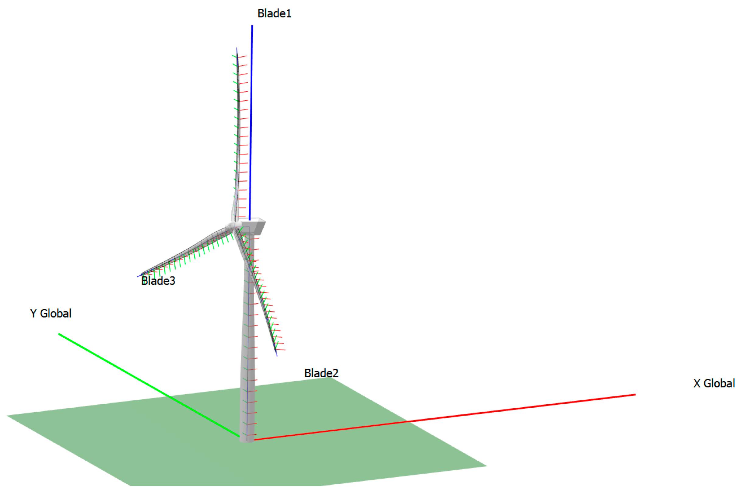
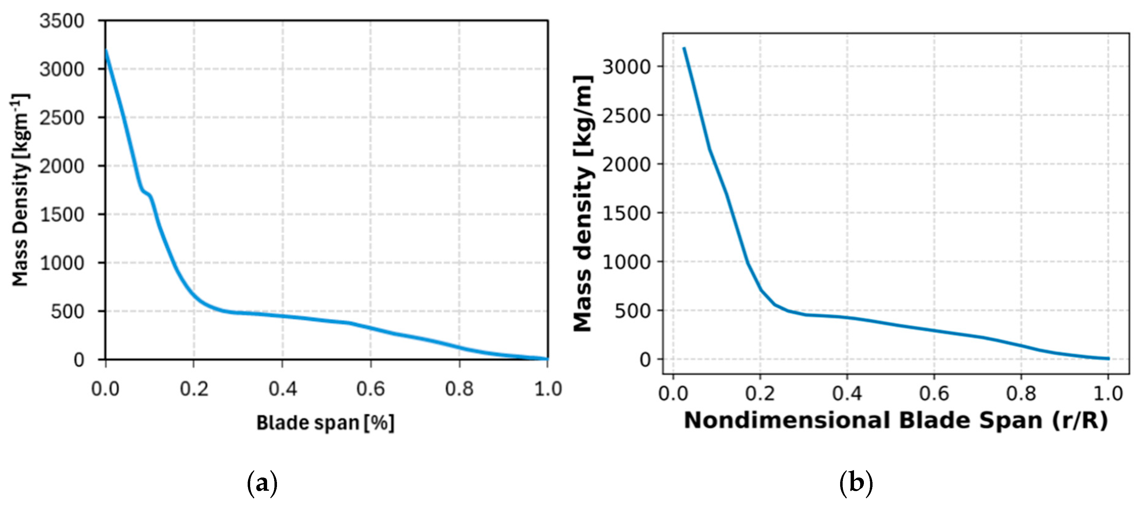
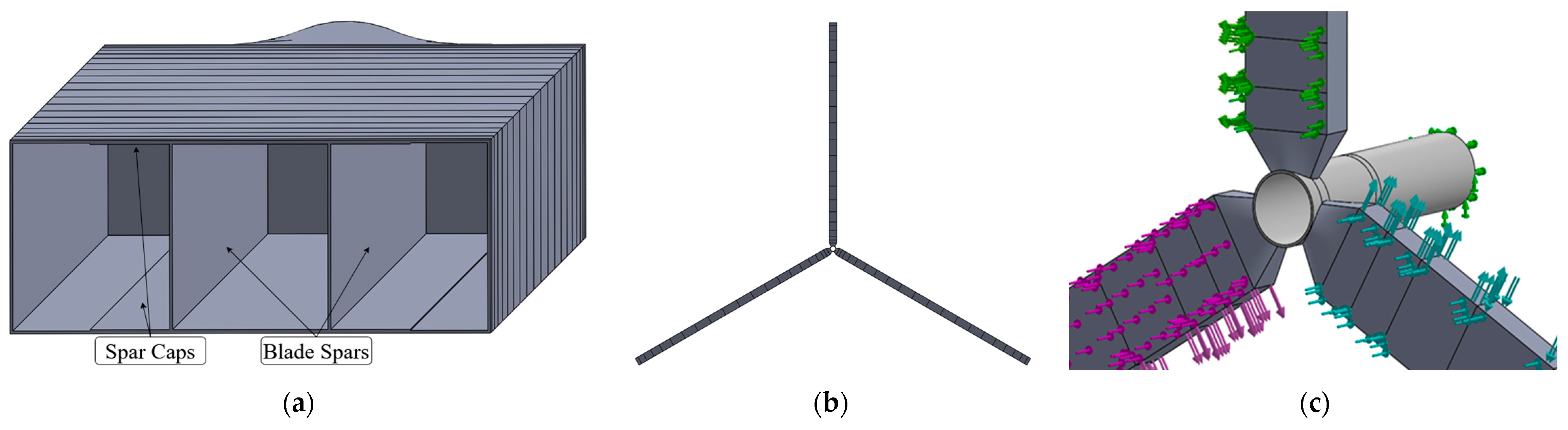
2.2. Simplified IEA-15MW-RWT Model Development in QBlade
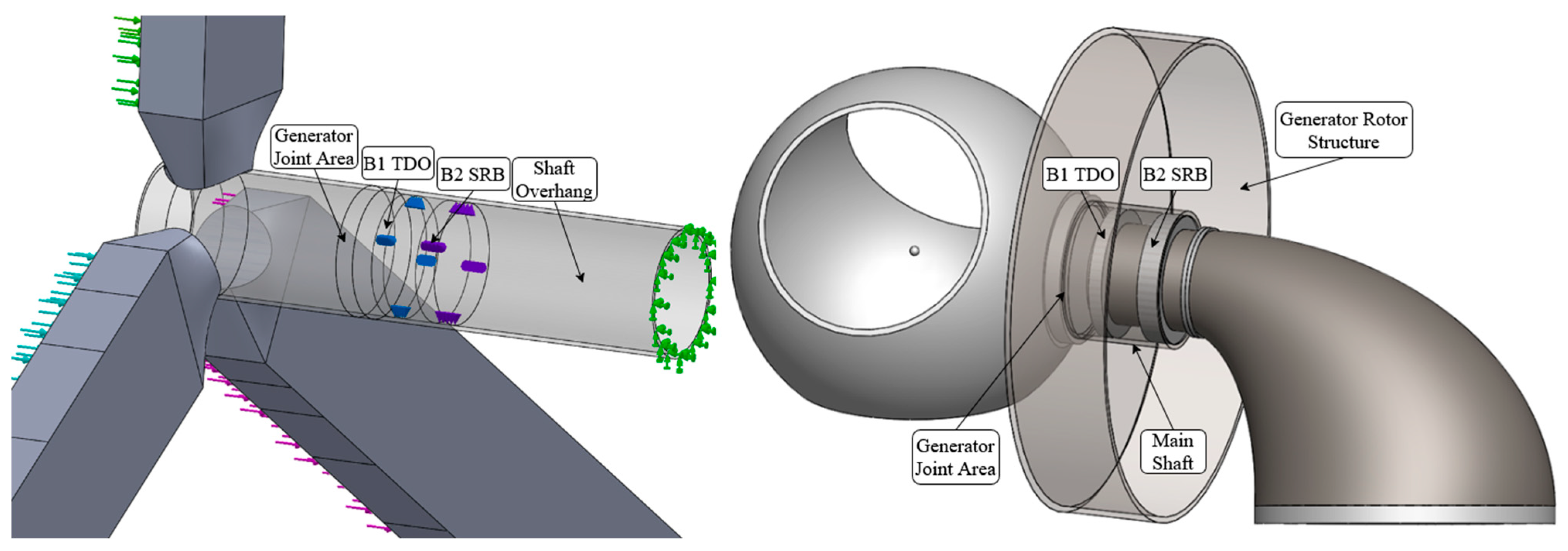
2.3. Simplified Drivetrain Model
2.4. Bearing Stiffness Calculations
2.4.1. Raceway Stiffness
2.4.2. Stiffness of Rolling Elements
2.4.3. Validation of Bearing Stiffnesses
2.5. Parametric Optimisation of the Generator Rotor
2.6. Governing Equations
2.6.1. Generator Power
2.6.2. Bearing Stiffness Calculation
2.6.3. Bearing Stiffness Validation
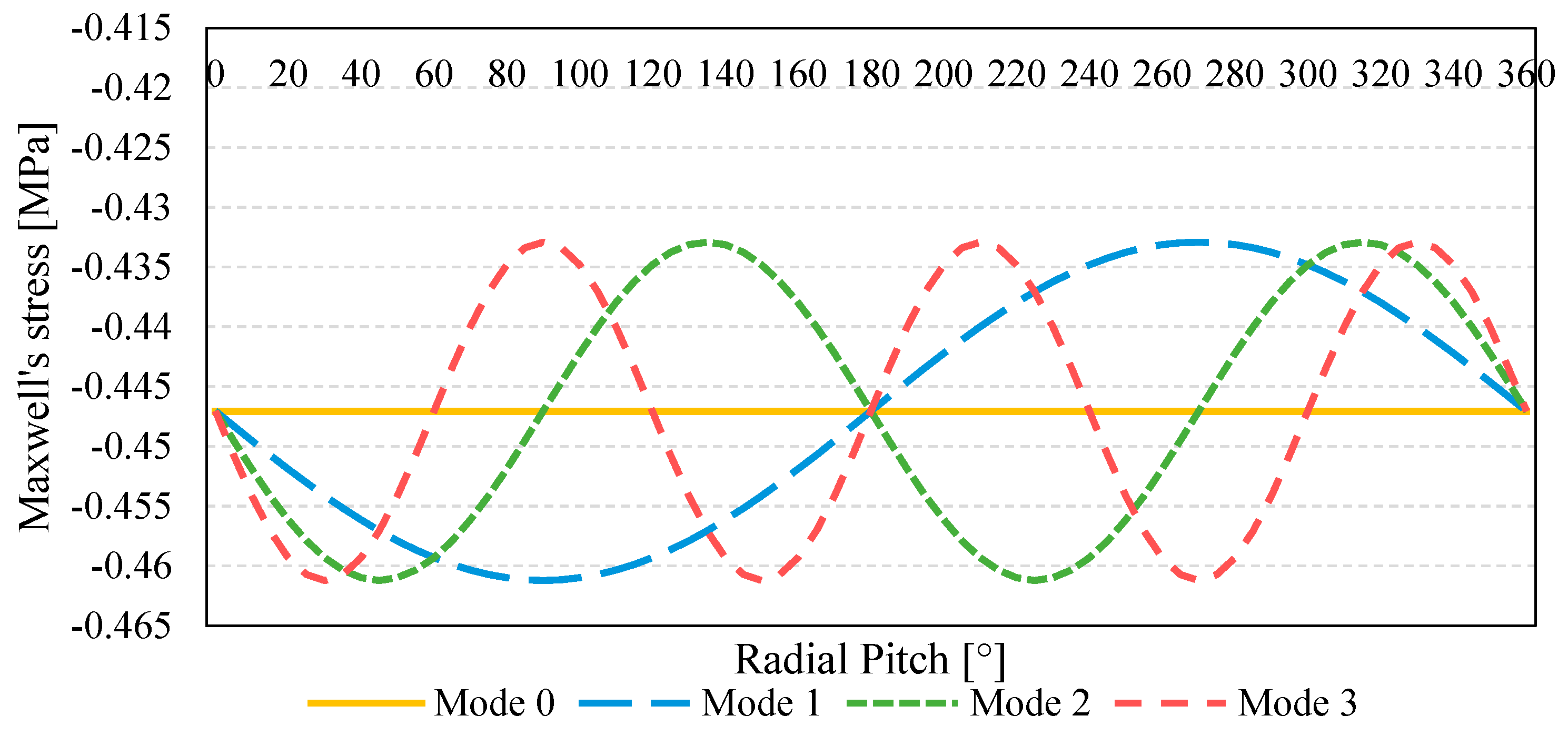
2.6.4. Modal Loading
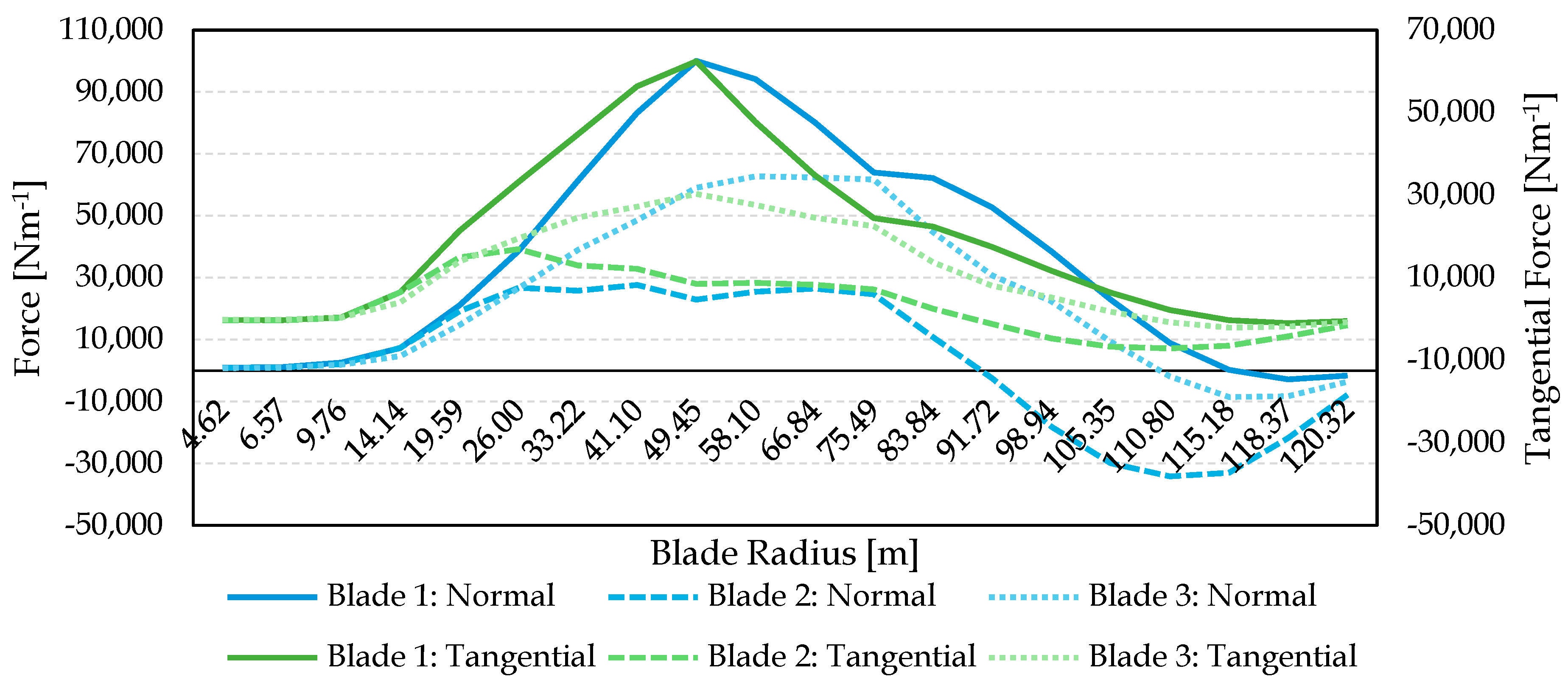
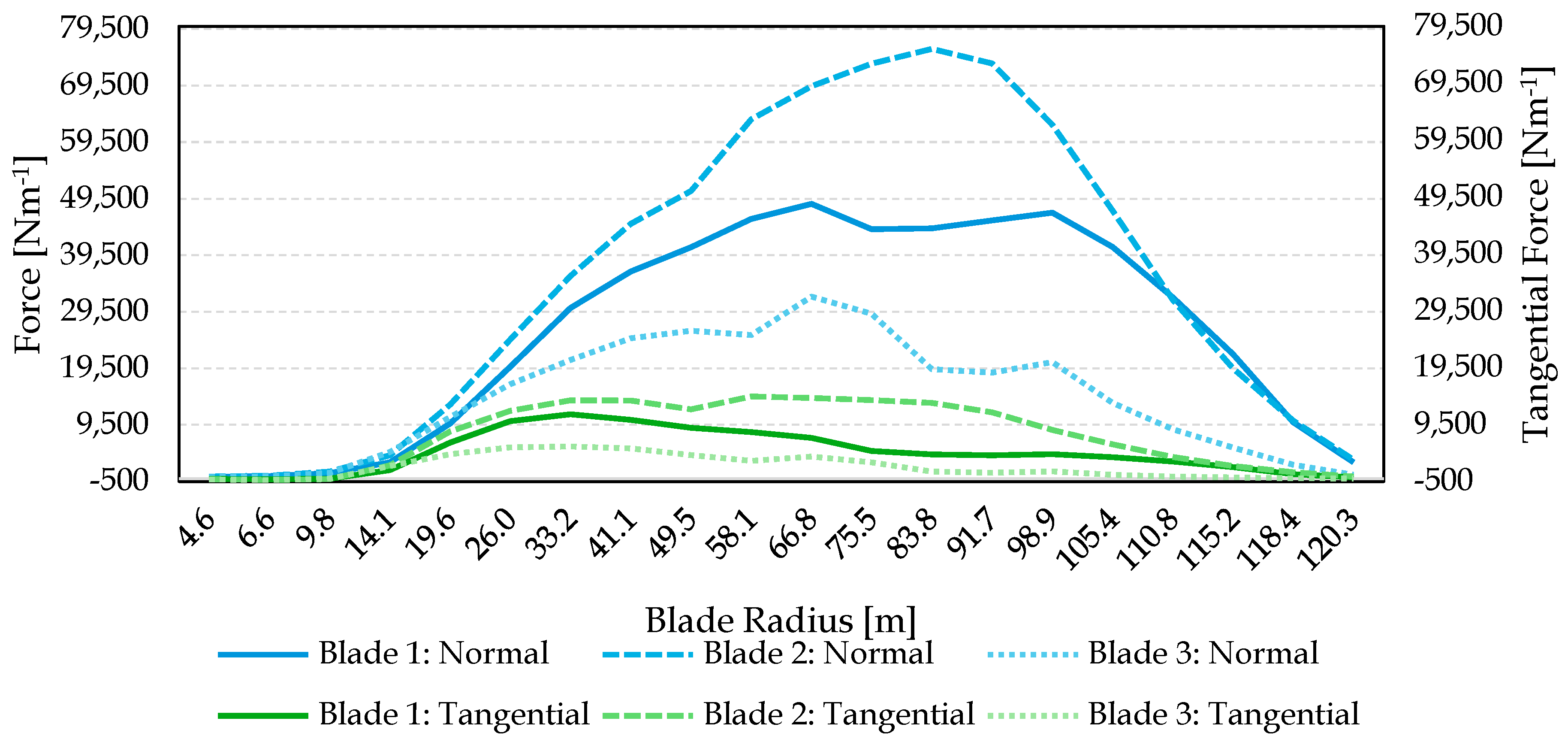
3. Results
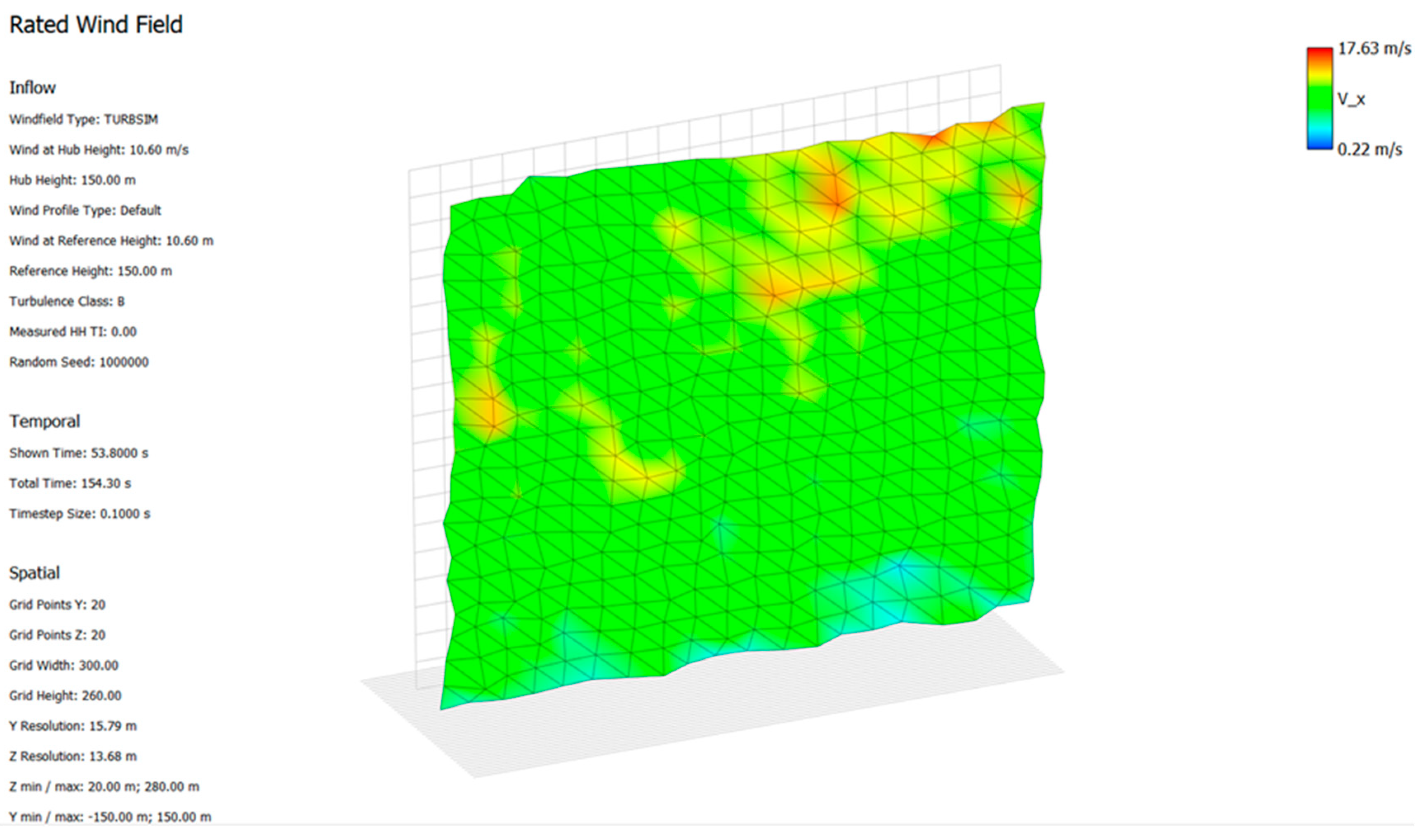
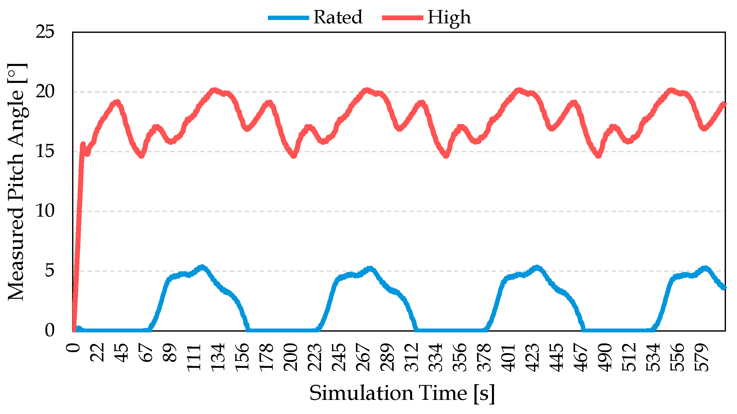
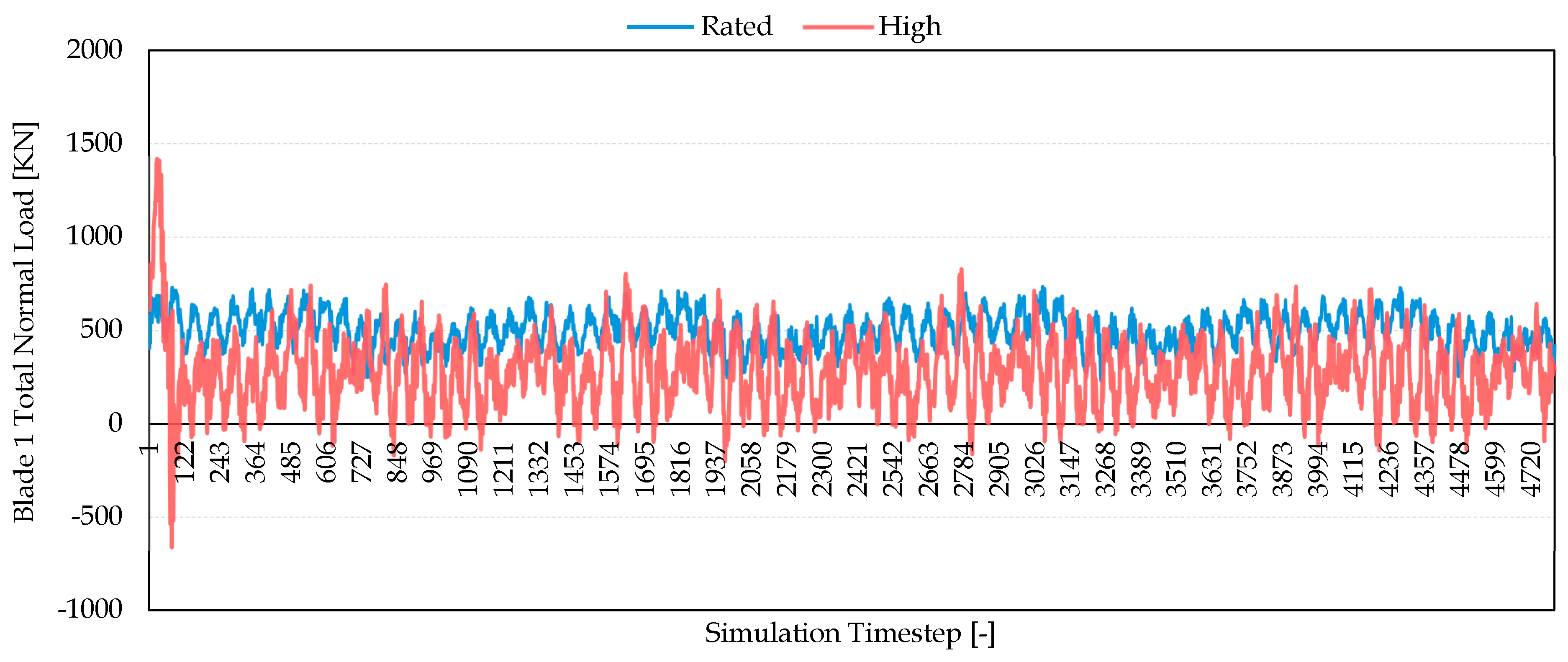
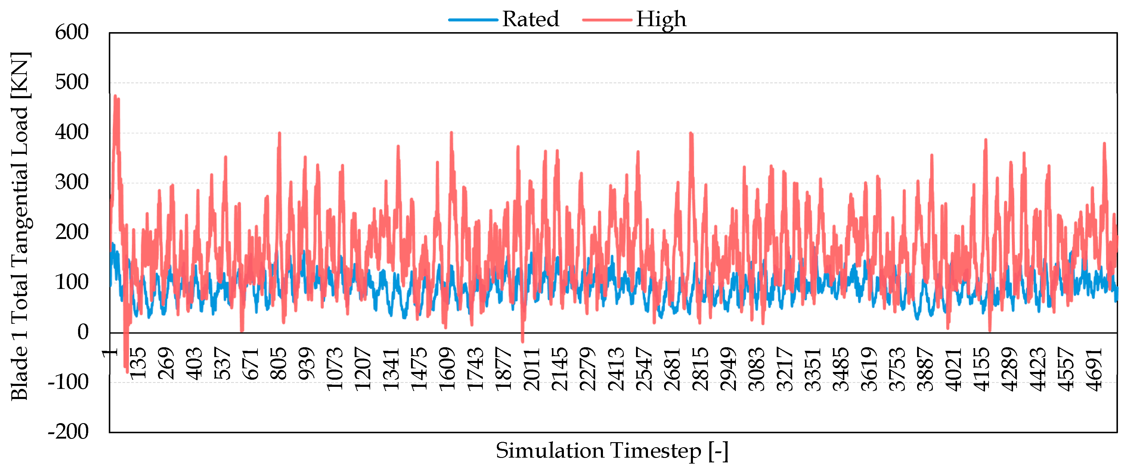
3.1. Aero-Servo-Elastic Simulation Results
- Final simulation timestep;
- Highest total normal load across rotor;
- Highest total tangential load across rotor;
- Highest combined normal and tangential load across rotor;
- Greatest normal rotor load imbalance;
- Greatest tangential rotor load imbalance.
3.1.1. Mesh Independence Study
3.1.2. Load Transfer Structural Analysis
3.2. Comparison of ASE Computational Analyses
3.3. Results of the Parametric Optimisation of the Generator Rotor
4. Discussion
5. Conclusions
Author Contributions
Funding
Data Availability Statement
Acknowledgments
Conflicts of Interest
Abbreviations
| O&M | Operation and Maintenance |
| LCOE | Levelised Cost of Energy |
| PMDD | Permanent Magnet Direct-Drive |
| IEA-15MW-RWT | International Energy Agency 15MW Reference Wind Turbine |
| FEA | Finite Element Analysis |
| CAD | Computer-Aided Design |
| HAWT | Horizontal Axis Wind Turbine |
| U-BEM | Unsteady Blade Element Momentum |
| TDO | Tapered Double Outer |
| SRB | Spherical Roller Bearing |
| B1_TDO | Bearing 1 (Tapered Double Outer) |
| B2_SRB | Bearing 2 (Spherical Roller Bearing) |
Appendix A

| IEA−15MW-RWT Blade Configuration | QBlade Blade Parameters | ||||||||||
|---|---|---|---|---|---|---|---|---|---|---|---|
| Diameter [m] | Chord [m] | Twist [deg] | X Axis Offset [m] | Y Axis Offset [m] | Position [m] | Chord [m] | Twist [deg] | IP Offset [m] | OOP Offset [m] | Foil | |
| 1 | 3.970 | 5.2000 | 15.5946 | −0.0228 | −0.0063 | 0.00000 | 5.20000 | 15.59 | −0.0228 | −0.0063 | AF00 |
| 2 | 6.358 | 5.2088 | 15.5877 | 0.0501 | 0.0324 | 2.38775 | 5.20884 | 15.59 | 0.0501 | 0.0324 | AF01 |
| 3 | 8.746 | 5.2379 | 15.4108 | 0.0869 | 0.0662 | 4.77551 | 5.23789 | 15.41 | 0.0869 | 0.0662 | AF02 |
| 4 | 11.133 | 5.2933 | 14.9486 | 0.0531 | 0.0855 | 7.16326 | 5.29333 | 14.95 | 0.0531 | 0.0855 | AF03 |
| 5 | 13.521 | 5.3673 | 14.2585 | −0.0283 | 0.0964 | 9.55101 | 5.36734 | 14.26 | −0.0283 | 0.0964 | AF04 |
| 6 | 15.909 | 5.4521 | 13.3971 | −0.1353 | 0.1050 | 11.93877 | 5.45209 | 13.40 | −0.1353 | 0.1050 | AF05 |
| 7 | 18.297 | 5.5400 | 12.4220 | −0.2434 | 0.1160 | 14.32652 | 5.54003 | 12.42 | −0.2434 | 0.1160 | AF06 |
| 8 | 20.684 | 5.6218 | 11.3946 | −0.3189 | 0.1340 | 16.71428 | 5.62182 | 11.39 | −0.3189 | 0.1340 | AF07 |
| 9 | 23.072 | 5.6925 | 10.3710 | −0.3470 | 0.1600 | 19.10203 | 5.69253 | 10.37 | −0.3470 | 0.1600 | AF08 |
| 10 | 25.460 | 5.7426 | 9.4040 | −0.3819 | 0.1773 | 21.48978 | 5.74261 | 9.40 | −0.3819 | 0.1773 | AF09 |
| 11 | 27.848 | 5.7648 | 8.5515 | −0.4163 | 0.1863 | 23.87754 | 5.76484 | 8.55 | −0.4163 | 0.1863 | AF10 |
| 12 | 30.235 | 5.7561 | 7.8332 | −0.4350 | 0.1904 | 26.26529 | 5.75612 | 7.83 | −0.4350 | 0.1904 | AF11 |
| 13 | 32.623 | 5.7031 | 7.1914 | −0.4193 | 0.1965 | 28.65304 | 5.70310 | 7.19 | −0.4193 | 0.1965 | AF12 |
| 14 | 35.011 | 5.6047 | 6.5516 | −0.3833 | 0.2035 | 31.04080 | 5.60468 | 6.55 | −0.3833 | 0.2035 | AF13 |
| 15 | 37.399 | 5.4716 | 5.9340 | −0.3521 | 0.2082 | 33.42855 | 5.47156 | 5.93 | −0.3521 | 0.2082 | AF14 |
| 16 | 39.786 | 5.3228 | 5.3461 | −0.3259 | 0.2108 | 35.81631 | 5.32278 | 5.35 | −0.3259 | 0.2108 | AF15 |
| 17 | 42.174 | 5.1665 | 4.7963 | −0.3029 | 0.2116 | 38.20406 | 5.16648 | 4.80 | −0.3029 | 0.2116 | AF16 |
| 18 | 44.562 | 5.0194 | 4.2966 | −0.2833 | 0.2111 | 40.59181 | 5.01942 | 4.30 | −0.2833 | 0.2111 | AF17 |
| 19 | 46.950 | 4.8858 | 3.8470 | −0.2650 | 0.2075 | 42.97957 | 4.88581 | 3.85 | −0.2650 | 0.2075 | AF18 |
| 20 | 49.337 | 4.7680 | 3.4453 | −0.2469 | 0.1961 | 45.36732 | 4.76796 | 3.45 | −0.2469 | 0.1961 | AF19 |
| 21 | 51.725 | 4.6546 | 3.0769 | −0.2287 | 0.1739 | 47.75507 | 4.65457 | 3.08 | −0.2287 | 0.1739 | AF20 |
| 22 | 54.113 | 4.5410 | 2.7336 | −0.2109 | 0.1379 | 50.14283 | 4.54103 | 2.73 | −0.2109 | 0.1379 | AF21 |
| 23 | 56.501 | 4.4282 | 2.4122 | −0.1945 | 0.0903 | 52.53058 | 4.42818 | 2.41 | −0.1945 | 0.0903 | AF22 |
| 24 | 58.888 | 4.3170 | 2.1117 | −0.1806 | 0.0345 | 54.91834 | 4.31696 | 2.11 | −0.1806 | 0.0345 | AF23 |
| 25 | 61.276 | 4.2079 | 1.8284 | −0.1687 | −0.0277 | 57.30609 | 4.20788 | 1.83 | −0.1687 | −0.0277 | AF24 |
| 26 | 63.664 | 4.1016 | 1.5588 | −0.1591 | −0.0932 | 59.69384 | 4.10165 | 1.56 | −0.1591 | −0.0932 | AF25 |
| 27 | 66.052 | 3.9987 | 1.3024 | −0.1520 | −0.1624 | 62.08160 | 3.99871 | 1.30 | −0.1520 | −0.1624 | AF26 |
| 28 | 68.439 | 3.8994 | 1.0644 | −0.1475 | −0.2435 | 64.46935 | 3.89941 | 1.06 | −0.1475 | −0.2435 | AF27 |
| 29 | 70.827 | 3.8032 | 0.8434 | −0.1443 | −0.3388 | 66.85710 | 3.80317 | 0.84 | −0.1443 | −0.3388 | AF28 |
| 30 | 73.215 | 3.7094 | 0.6366 | −0.1429 | −0.4485 | 69.24486 | 3.70939 | 0.64 | −0.1429 | −0.4485 | AF29 |
| 31 | 75.603 | 3.6171 | 0.4370 | −0.1431 | −0.5692 | 71.63261 | 3.61711 | 0.44 | −0.1431 | −0.5692 | AF30 |
| 32 | 77.990 | 3.5256 | 0.2397 | −0.1449 | −0.6981 | 74.02036 | 3.52563 | 0.24 | −0.1449 | −0.6981 | AF31 |
| 33 | 80.378 | 3.4341 | 0.0397 | −0.1477 | −0.8322 | 76.40812 | 3.43408 | 0.04 | −0.1477 | −0.8322 | AF32 |
| 34 | 82.766 | 3.3419 | −0.1728 | −0.1512 | −0.9695 | 78.79587 | 3.34193 | −0.17 | −0.1512 | −0.9695 | AF33 |
| 35 | 85.154 | 3.2487 | −0.4071 | −0.1552 | −1.1080 | 81.18363 | 3.24868 | −0.41 | −0.1552 | −1.1080 | AF34 |
| 36 | 87.541 | 3.1561 | −0.6804 | −0.1596 | −1.2532 | 83.57138 | 3.15611 | −0.68 | −0.1596 | −1.2532 | AF35 |
| 37 | 89.929 | 3.0646 | −0.9993 | −0.1642 | −1.4075 | 85.95913 | 3.06458 | −1.00 | −0.1642 | −1.4075 | AF36 |
| 38 | 92.317 | 2.9730 | −1.3205 | −0.1685 | −1.5694 | 88.34689 | 2.97299 | −1.32 | −0.1685 | −1.5694 | AF37 |
| 39 | 94.705 | 2.8807 | −1.6233 | −0.1724 | −1.7386 | 90.73464 | 2.88071 | −1.62 | −0.1724 | −1.7386 | AF38 |
| 40 | 97.092 | 2.7870 | −1.8844 | −0.1755 | −1.9137 | 93.12239 | 2.78697 | −1.88 | −0.1755 | −1.9137 | AF39 |
| 41 | 99.480 | 2.6910 | −2.0862 | −0.1785 | −2.0936 | 95.51015 | 2.69103 | −2.09 | −0.1785 | −2.0936 | AF40 |
| 42 | 101.868 | 2.5920 | −2.1640 | −0.1819 | −2.2786 | 97.89790 | 2.59197 | −2.16 | −0.1819 | −2.2786 | AF41 |
| 43 | 104.256 | 2.4893 | −2.1758 | −0.1856 | −2.4686 | 100.28566 | 2.48932 | −2.18 | −0.1856 | −2.4686 | AF42 |
| 44 | 106.643 | 2.3839 | −2.1553 | −0.1893 | −2.6663 | 102.67341 | 2.38392 | −2.16 | −0.1893 | −2.6663 | AF43 |
| 45 | 109.031 | 2.2759 | −2.1029 | −0.1925 | −2.8712 | 105.06116 | 2.27592 | −2.10 | −0.1925 | −2.8712 | AF44 |
| 46 | 111.419 | 2.1655 | −2.0184 | −0.1950 | −3.0832 | 107.44892 | 2.16547 | −2.02 | −0.1950 | −3.0832 | AF45 |
| 47 | 113.807 | 2.0526 | −1.8967 | −0.1971 | −3.3019 | 109.83667 | 2.05263 | −1.90 | −0.1971 | −3.3019 | AF46 |
| 48 | 116.194 | 1.9378 | −1.7243 | −0.1990 | −3.5277 | 112.22442 | 1.93775 | −1.72 | −0.1990 | −3.5277 | AF47 |
| 49 | 118.582 | 1.8197 | −1.5081 | −0.2003 | −3.7589 | 114.61218 | 1.81966 | −1.51 | −0.2003 | −3.7589 | AF48 |
| 50 | 120.970 | 0.5000 | −1.2424 | −0.0591 | −3.9987 | 116.99993 | 0.50000 | −1.24 | −0.0591 | −3.9987 | AF49 |

References
- BloombergNEF Global Low-Carbon Energy Technology Investment Surges Past $1 Trillion for the First Time. BNEF 2023. Available online: https://about.bnef.com/blog/global-low-carbon-energy-technology-investment-surges-past-1-trillion-for-the-first-time/ (accessed on 11 June 2024).
- Costanzo, G.; Brindley, G.; Willems, G.; Ramirez, L.; Cope, P.; Klonari, V. Wind Energy in Europe: 2023 Statistics and the Outlook for 2024–2030; O’Sullivan, R., Ed.; WindEurope: Brussels, Belgium, 2024. [Google Scholar]
- Department for Energy Security & Net Zero. Electricity Generation Costs 2023; Department for Energy Security & Net Zero: London, UK, 2023. Available online: https://assets.publishing.service.gov.uk/media/6556027d046ed400148b99fe/electricity-generation-costs-2023.pdf (accessed on 28 April 2024).
- Kaiser, M.J.; Snyder, B.F. Offshore Wind Energy Cost Modeling; Springer: London, UK, 2012; ISBN 9781608054220. [Google Scholar]
- DESNZ Renewable Energy Planning Database (REPD): July 2024. Available online: https://www.gov.uk/government/publications/renewable-energy-planning-database-monthly-extract (accessed on 16 August 2024).
- BEIS. Renewable Energy Planning Database (REPD): April 2023; BEIS: London, UK, 2023. Available online: https://www.gov.uk/government/publications/renewable-energy-planning-database-monthly-extract (accessed on 3 July 2023).
- Durakovic, A. First Siemens Gamesa 14.7 MW Turbine Stands at Moray West Offshore Wind Farm. Offshore WIND 2024. Available online: https://www.offshorewind.biz/2024/04/22/first-siemens-gamesa-14-7-mw-turbine-stands-at-moray-west-offshore-wind-farm/ (accessed on 10 May 2024).
- GE Vernova GE’s Haliade-X 14.7 MW-220 Turbine Obtains Full DNV Type Certificate 2022. Available online: https://www.ge.com/news/taxonomy/term/2152 (accessed on 11 September 2024).
- Nield, D. The Largest and Most Powerful Wind Turbine Ever Built Is Now Operational. ScienceAlert 2023. Available online: https://www.sciencealert.com/the-largest-and-most-powerful-wind-turbine-ever-built-is-now-operational (accessed on 2 May 2024).
- Ren, Z.; Verma, A.S.; Li, Y.; Teuwen, J.J.; Jiang, Z. Offshore Wind Turbine Operations and Maintenance: A State-of-the-Art Review. Renew. Sustain. Energy Rev. 2021, 144, 110886. [Google Scholar] [CrossRef]
- Nejad, A.R.; Keller, J.; Guo, Y.; Sheng, S.; Polinder, H.; Watson, S.; Dong, J.; Qin, Z.; Ebrahimi, A.; Schelenz, R.; et al. Wind Turbine Drivetrains: State-of-the-Art Technologies and Future Development Trends. Wind Energy Sci. 2022, 7, 387–411. [Google Scholar] [CrossRef]
- Dalgic, Y.; Lazakis, I.; Turan, O. Vessel Charter Rate Estimation for Offshore Wind O&M Activities. In Proceedings of the 15th International Congress of the International Maritime Association of the Mediterranean IMAM, Coruna, Spain, 14–17 October 2013; pp. 899–908. [Google Scholar]
- Dao, C.; Kazemtabrizi, B.; Crabtree, C. Wind Turbine Reliability Data Review and Impacts on Levelised Cost of Energy. Wind Energy 2019, 22, 1655–1890. [Google Scholar] [CrossRef]
- Hayes, A.; Sethuraman, L.; Dykes, K.; Fingersh, L.J. Structural Optimization of a Direct-Drive Wind Turbine Generator Inspired by Additive Manufacturing. Procedia Manuf. 2018, 26, 740–752. [Google Scholar] [CrossRef]
- Hayes, A.C.; Whiting, G.L. Reducing the Structural Mass of Large Direct Drive Wind Turbine Generators through Triply Periodic Minimal Surfaces Enabled by Hybrid Additive Manufacturing. Clean Technol. 2021, 3, 227–242. [Google Scholar] [CrossRef]
- Tartt, K.; Amiri, A.K.; McDonald, A.; Jaen-Sola, P. Structural Optimisation of Offshore Direct-Drive Wind Turbine Generators Including Static and Dynamic Analyses. J. Phys. Conf. Ser. 2021, 2018, 012040. [Google Scholar] [CrossRef]
- Jaen-Sola, P.; Oterkus, E.; McDonald, A.S. Parametric Lightweight Design of a Direct-Drive Wind Turbine Electrical Generator Supporting Structure for Minimising Dynamic Response. Ships Offshore Struct. 2021, 16, 266–274. [Google Scholar] [CrossRef]
- Marten, D.; Saverin, J.; Perez-Becker, S.; Behrens de Luna, R. QBlade CE 2023 (v 2.0.5.1). Available online: https://qblade.org/ (accessed on 10 April 2023).
- BOVIA Dassault Systèmes. BOVIA Solidworks; 2022 (v 29.3.0.0059). Available online: https://www.solidworks.com/ (accessed on 10 April 2023).
- Szatkowski, S.; Jaen-Sola, P.; Oterkus, E. An Efficient Computational Analysis and Modelling of Transferred Aerodynamic Loading on Direct-Drive System of 5 MW Wind Turbine and Results Driven Optimisation for a Sustainable Generator Structure. Sustainability 2024, 16, 545. [Google Scholar] [CrossRef]
- Gaertner, E.; Rinker, J.; Sethuraman, L.; Zahle, F.; Anderson, B.; Barter, G.; Skrzypinski, W. Definition of the IEA 15 MW Offshore Reference Wind Turbine; National Renewable Energy Laboratory. NREL/TP-5000-75698: Golden, CO, USA, 2020. Available online: https://docs.nrel.gov/docs/fy20osti/75698.pdf (accessed on 9 January 2023).
- Ghafoorian, F.; Enayati, E.; Mirmotahari, S.R.; Wan, H. Self-Starting Improvement and Performance Enhancement in Darrieus VAWTs Using Auxiliary Blades and Deflectors. Machines 2024, 12, 806. [Google Scholar] [CrossRef]
- Ghafoorian, F.; Wan, H.; Chegini, S. A Systematic Analysis of a Small-Scale HAWT Configuration and Aerodynamic Performance Optimization Through Kriging, Factorial, and RSM Methods. J. Appl. Comput. Mech 2024, 3, 1–17. [Google Scholar] [CrossRef]
- Glauert, H. Aerodynamic Theory. Chapter 3: Airplane Propellers, 1st ed.; Springer: Berlin/Heidelberg, Germany, 1935; ISBN 978-3-642-91487-4. [Google Scholar]
- Snel, H.; Houwink, R.; Piers, W.J. Sectional Prediction of 3D Effects for Separated Flow on Rotating Blades. In Proceedings of the Eighteenth European Rotorcraft Forum, National Aerospace Laboratory, NL, Avignon, France, 21 September 1992. [Google Scholar]
- Gaertner, E.; Rinker, J.; Sethuraman, L.; Zahle, F.; Anderson, B.; Barter, G.; Abbas, N.; Meng, F.; Bortolotti, P.; Skrzypinski, W.; et al. IEA-15-240-RWT: 15MW Reference Wind Turbine Repository; 2020. Available online: https://github.com/IEAWindSystems/IEA-15-240-RWT (accessed on 10 April 2023).
- Hansen, M.H.; Henriksen, L.C. Basic DTU Wind Energy Controller; DTU Wind Energy: Roskilde, Denmark, 2013; ISBN 9788792896278. [Google Scholar]
- Kelley, N.; Jonkman, B. TurbSim; NREL 2012. Available online: https://www.nrel.gov/wind/nwtc/turbsim.html (accessed on 25 January 2024).
- Toupin, R.A. On St. Venet’s Principle. In Proceedings of the Applied Mechanics; Springer: Berlin/Heidelberg, Germany, 1966; pp. 151–152. [Google Scholar]
- Sethuraman, L.; Xing, Y.; Venugopal, V.; Gao, Z.; Mueller, M.; Moan, T. A 5 MW Direct-Drive Generator for Floating Spar-Buoy Wind Turbine: Drive-Train Dynamics. Proc. Inst. Mech. Eng. C J. Mech. Eng. Sci. 2017, 231, 744–763. [Google Scholar] [CrossRef]
- Zhang, H.; Shi, W.; Liu, G.; Chen, Z. A Method to Solve the Stiffness of Double-Row Tapered Roller Bearing. Math. Probl. Eng. 2019, 2019. [Google Scholar] [CrossRef]
- Zhang, F.; Lv, H.; Han, Q.; Li, M. The Effects Analysis of Contact Stiffness of Double-Row Tapered Roller Bearing under Composite Loads. Sensors 2023, 23, 4967. [Google Scholar] [CrossRef] [PubMed]
- SKF. SKF® Product Catalogue: Rolling Bearings. Available online: https://www.skf.com/uk/products/rolling-bearings (accessed on 14 December 2023).
- Gargiulo, E.P., Jr. A Simple Way to Estimate Bearing Stiffness. Mach. Des. 1980, 52, 107–110. [Google Scholar]
- Allen, C.; Viselli, A.; Dagher, H.; Goupee, A.; Gaertner, E.; Abbas, N.; Hall, M.; Barter, G. Definition of the UMaine VolturnUS-S Reference Platform Developed for the IEA Wind 15-Megawatt Offshore Reference Wind Turbine; National Renewable Energy Laboratory. NREL/TP-5000-76773: Golden, CO, USA, 2020. [Google Scholar]
- Bichan, M.; Jaen-Sola, P.; Sellami, N.; Muhammad-Sukki, F. Aero-Servo-Elastic Simulation of the International Energy Agency’s 15MW Reference Wind Turbine for Direct-Drive Generator Integrity Modelling. In Proceedings of the ASWEC 2024, Edinburgh, Scotland, UK, 31 July 2024. [Google Scholar]
- Sethuraman, L.; Venugopal, V.; Zavvos, A.; Mueller, M. Structural Integrity of a Direct-Drive Generator for a Floating Wind Turbine. Renew. Energy 2014, 63, 597–616. [Google Scholar] [CrossRef]
- Zahle, F.; Barlas, A.; Lønbaek, K.; Bortolotti, P.; Zalkind, D.; Wang, L.; Labuschagne, C.; Sethuraman, L.; Barter, G. Definition of the IEA Wind 22-Megawatt Offshore Reference Wind Turbine; Technical University of Denmark (DTU), Department of Wind and Energy Systems: Roskilde, Denmark, 2024. [Google Scholar] [CrossRef]


| Material Property | Value | Units |
|---|---|---|
| Elastic Modulus | 7.30 × 10¹⁰ | Nm−2 |
| Poisson’s Ratio | 2.00 × 10⁻¹ | - |
| Shear Modulus | 3.00 × 10⁹ | Nm−2 |
| Mass Density | 2.90 × 10³ | kgm−3 |
| Tensile Strength | 1.24 × 10⁸ | Nm−2 |
| Yield Strength | 4.20 × 10⁸ | Nm−2 |
| Material Property | Value | Units |
|---|---|---|
| Elastic Modulus | 2.03 × 10¹¹ | Nm−2 |
| Poisson’s Ratio | 3.00 × 10⁻¹ | - |
| Shear Modulus | 7.82 × 10¹⁰ | Nm−2 |
| Mass Density | 7.825 × 10³ | kgm−3 |
| Tensile Strength | 4.48 × 10⁸ | Nm−2 |
| Yield Strength | 2.34 × 10⁸ | Nm−2 |
| Blade Property | Value | Shaft Property | Value |
|---|---|---|---|
| Length | 117 m | Length | 13.075 m |
| Depth | 1628 mm | Shaft outer diameter | 3000 mm |
| Width | 4050 mm | Shaft inner diameter | 2800 mm |
| Shell thickness | 23.61 mm | Bearing outer diameter | 2800 mm |
| Spar width | 25 mm | Bearing inner diameter | 2200 mm |
| Spar cap thickness | 10 mm | B1_TDO width | 300 mm |
| Spar centroid distance to inside wall | 1334.26 mm | B1_TDO distance to rotor inner face | 433.5 mm |
| Spar cap width | 2700 mm | B2_SRB width | 470 mm |
| Blade root distance to shaft | 3000 mm | B2_SRB distance to rotor inner face | 1548.5 mm |
| Blade mounting disc diameter | 2000 mm | Shaft overhang length from B2_SRB | 7565.32 mm |
| Blade Property | Original Values | Reduced Values |
|---|---|---|
| Length | 117 m | 117 m |
| Depth | 1628 mm | 1628 mm |
| Width | 4050 mm | 4050 mm |
| Shell thickness: top and bottom | 23.61 mm | 23.61 |
| Shell thickness: side walls | 23.61 mm | 17.71 mm |
| Spar width | 25 mm | 12.5 mm |
| Spar cap thickness | 10 mm | 8 mm |
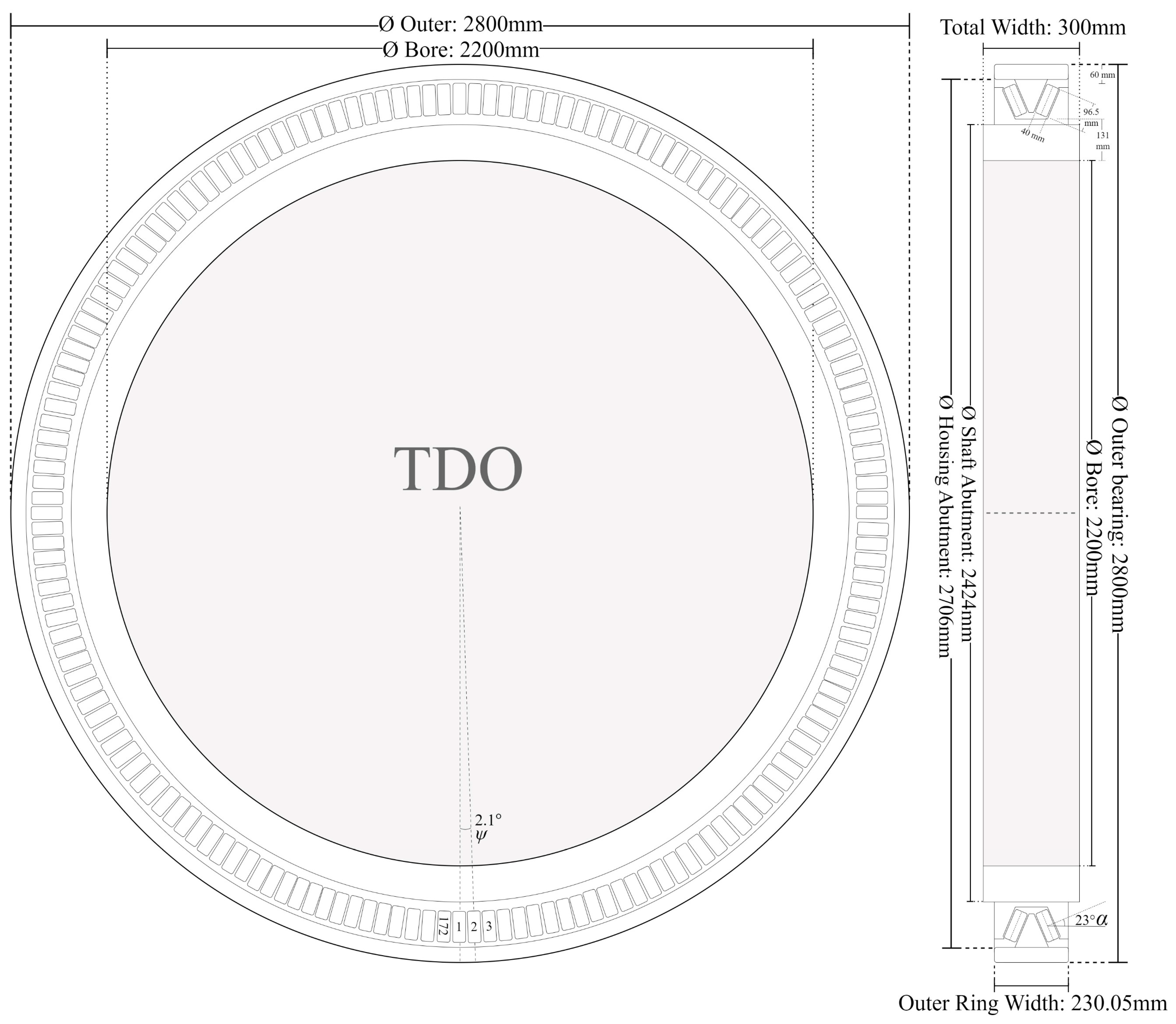
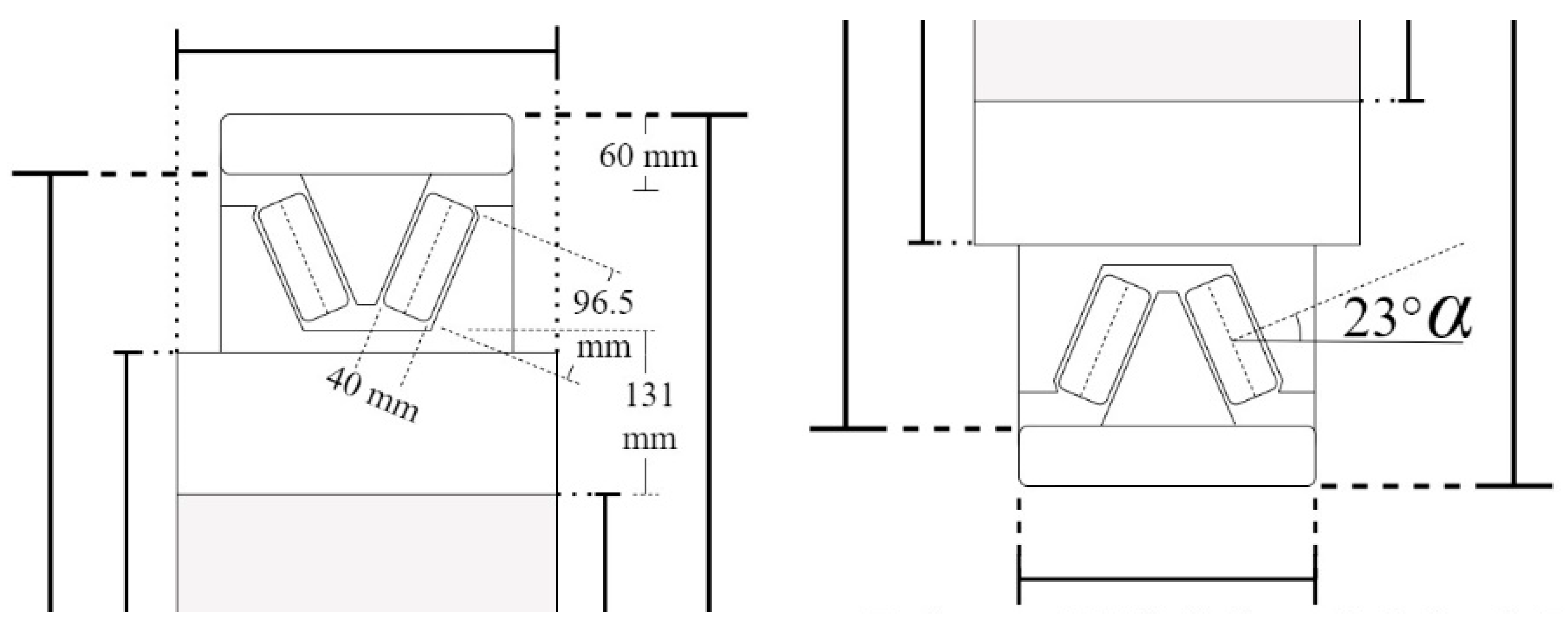
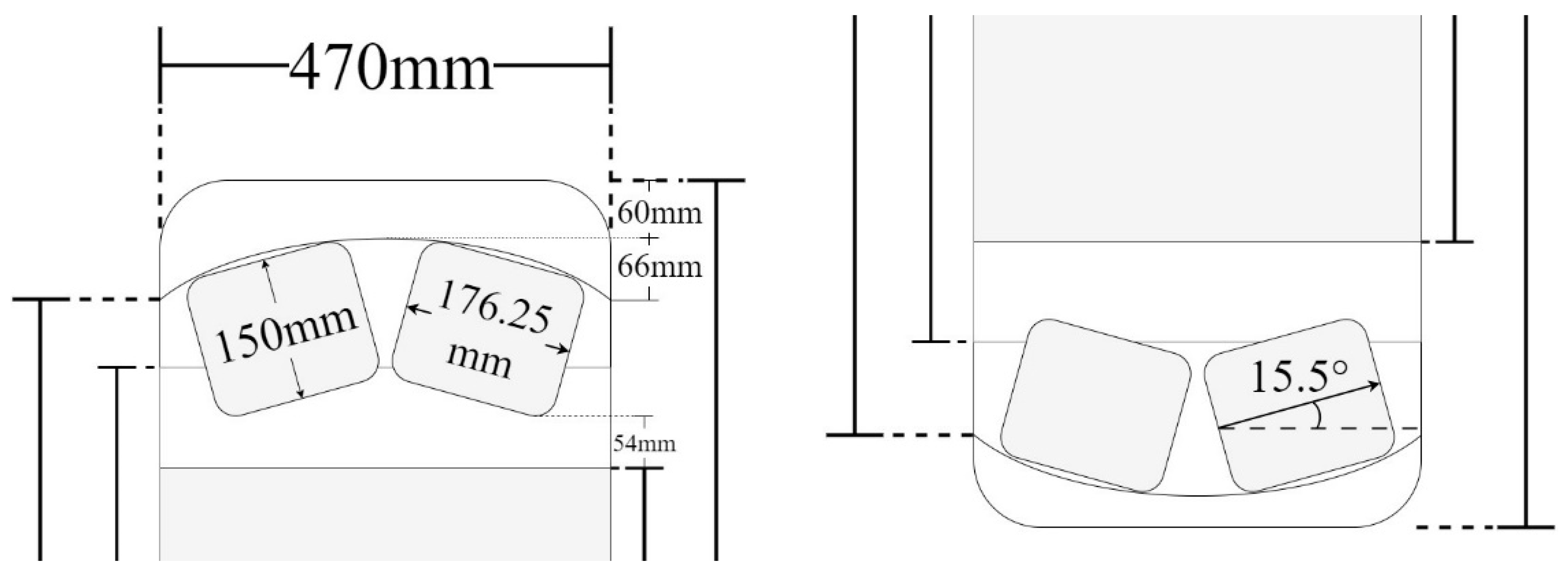
| 3 Bore Diameter [mm] | 3 Outside Diameter [mm] | 2 Raceway Thickness [mm] | 1,3 Raceway Width [mm] | 2 Roller Lengths [mm] | 1 Roller Diam. [mm] | 1 Contact Angle [°] | 2 Roller Azimuth [°] | 2 Number of Rollers [-] | ||
|---|---|---|---|---|---|---|---|---|---|---|
| TDO | Outer | 2200 | 2800 | 65 | 230.05 (1) | 92.5 | 41 | 23 | 2.09 | 172 |
| Inner | - | - | 130 | 300 (3) | - | 40 | - | - | - | |
| SRB | Outer | 2200 | 2800 | 94.5 | 470 (3) | 176.25 | 150 | 15.5 | 7.2 | 50 |
| Inner | - | - | 78.75 | 470 (3) | - | - | - | - | - |
| Component | Bearing 1_TDO | Bearing 2_SRB | |
|---|---|---|---|
| Axial Stiffness [Nm−1] | Radial Stiffness [Nm−1] | Radial Stiffness [Nm−1] | |
| Inner raceway | 3.918 × 10¹¹ | 7.485 × 10¹³ | 1.101 × 10¹³ |
| Rolling element | 6.124 × 10¹⁰ | 1.021 × 10¹¹ | 3.968 × 10¹⁰ |
| Outer raceway | 4.734 × 10¹¹ | 1.339 × 10¹³ | 2.211 × 10¹³ |
| Bearing total | 4.763 × 10¹⁰ | 1.018 × 10¹¹ | 3.946 × 10¹⁰ |
| System total | 4.763 × 10¹⁰ | 1.413 × 10¹¹ | |
| Conditions | S1: Final Timestep | S2: Greatest Normal Load | S3: Greatest Tang. Load | S4: Greatest Total Combined | S5: Largest Norm. Imbalance | S6: Largest Tang. Imbalance | Units | |
|---|---|---|---|---|---|---|---|---|
| Norm. Only | Norm. and Tang. | |||||||
| Max. Blade Displ. (Rigid) | −13.16 | −13.16 | −17.89 | −16.78 | −16.88 | −12.93 | −13.77 | m |
| Max. Blade Displ. (Flex.) | −13.17 | −13.16 | −17.90 | −16.78 | −16.88 | −12.94 | −13.78 | m |
| Max. Shaft Displ. (Rigid) | 9.943 | 11.603 | 15.521 | 14.911 | 15.288 | 14.225 | 15.169 | mm |
| Max. Shaft Displ. (Flex.) | 9.959 | 11.774 | 15.704 | 15.004 | 15.135 | 14.607 | 15.552 | mm |
| Max. Gen. Area Displ. (Rigid) | 1.233 | 2.111 | 2.190 | 2.430 | 2.219 | 1.737 | 1.829 | mm |
| Max. Gen. Area Displ. (Flex.) | 1.311 | 2.172 | 2.254 | 2.488 | 2.256 | 1.858 | 1.937 | mm |
| Max. Gen. Area Stress (Rigid) | 63.393 | 77.450 | 89.381 | 94.504 | 90.665 | 88.824 | 94.716 | MPa |
| Max. Gen. Area Stress (Flex.) | 63.335 | 77.442 | 89.465 | 94.569 | 90.593 | 88.837 | 94.727 | MPa |
| B1_TDO Max. Radial Stress (Flex.) | 15.315 | 16.872 | 21.585 | 19.893 | 17.980 | 17.023 | 18.171 | MPa |
| B2_SRB Max. Radial stress (Flex.) | 2.874 | 2.907 | 2.652 | 3.053 | 2.212 | 6.604 | 6.414 | MPa |
| Shaft Eccentricity (Rigid) | 12.1 | 20.8 | 21.6 | 23.9 | 21.9 | 17.1 | 18.0 | % |
| Shaft Eccentricity (Flex.) | 12.9 | 21.4 | 22.2 | 24.5 | 22.2 | 18.3 | 19.1 | % |
| New Limit (Rigid) | 1.783 | 1.608 | 1.592 | 1.544 | 1.586 | 1.683 | 1.664 | mm |
| New Limit (Flex.) | 1.768 | 1.596 | 1.579 | 1.532 | 1.579 | 1.658 | 1.643 | mm |
| Conditions | S1: Final Timestep | S4: Worst Total Combined Load | S5: Largest Normal Imbalance | S6: Largest Tangential Imbalance | Units | |
|---|---|---|---|---|---|---|
| Normal Only | Normal and Tang. | |||||
| Max. Blade Displacement (Rigid) | 0.58 | 1.19 | −27.49 | −13.90 | −9.48 | m |
| Max. Blade Displacement (Flex.) | 0.58 | 1.19 | −27.49 | −13.92 | −9.48 | m |
| Max. Shaft Displacement (Rigid) | 0.310 | 4.053 | 27.763 | 27.705 | 17.942 | mm |
| Max. Shaft Displacement (Flex.) | 0.323 | 4.136 | 28.007 | 28.617 | 18.445 | mm |
| Max. Gen. Area Displacement (Rigid) | 0.050 | 0.811 | 5.649 | 3.595 | 2.449 | mm |
| Max. Gen. Area Displacement (Flex.) | 0.055 | 0.835 | 5.722 | 3.924 | 2.613 | mm |
| Max. Gen. Area Stress (Rigid) | 2.150 | 26.511 | 190.942 | 166.628 | 125.784 | MPa |
| Max. Gen. Area Stress (Flex.) | 2.151 | 26.512 | 190.948 | 166.643 | 125.801 | MPa |
| B1_TDO Max. Radial Stress (Flex.) | 0.312 | 3.503 | 36.088 | 37.310 | 21.536 | MPa |
| B2_SRB Max. Radial Stress (Flex.) | 0.237 | 1.274 | 5.036 | 13.048 | 9.798 | MPa |
| Shaft Eccentricity (Rigid) | 0.005 | 0.080 | 0.557 | 0.354 | 0.241 | % |
| Shaft Eccentricity (Flex.) | 0.005 | 0.082 | 0.564 | 0.387 | 0.257 | % |
| New Limit (Rigid) | 2.020 | 1.868 | 0.900 | 1.311 | 1.540 | mm |
| New Limit (Flex.) | 2.019 | 1.863 | 0.886 | 1.245 | 1.507 | mm |
| S1: Final Timestep | S2: Greatest Total Normal Load | S5: Largest Normal Load Imbalance | |||||
|---|---|---|---|---|---|---|---|
| Conditions | Normal Only | Normal and Tang. | Normal Only | Normal and Tang. | Normal Only | Normal and Tang. | Units |
| Max. Blade Displacement | −13.17 | −13.16 | −17.88 | −17.90 | −12.95 | −12.94 | m |
| Max. Shaft Displacement | 9.959 | 11.774 | 13.507 | 15.704 | 13.525 | 14.607 | mm |
| Max. Gen. Area Displacement | 1.311 | 2.172 | 1.443 | 2.254 | 1.799 | 1.858 | mm |
| Max. Von Mises Gen. Area stress | 63.34 | 77.44 | 75.11 | 89.46 | 75.93 | 88.84 | MPa |
| B1_TDO Max. Radial Stress | 15.32 | 16.87 | 19.24 | 21.59 | 19.44 | 17.02 | MPa |
| B2_SRB Max. Radial stress | 2.87 | 2.91 | 2.68 | 2.65 | 6.50 | 6.60 | MPa |
| Shaft Eccentricity | 12.9 | 21.4 | 14.2 | 22.2 | 17.7 | 18.3 | % |
| New Limit | 1.768 | 1.596 | 1.741 | 1.579 | 1.670 | 1.658 | mm |
| S1: Final Timestep | S2(4): Greatest Total Normal (Combined) Load | S5: Largest Normal Load Imbalance | |||||
|---|---|---|---|---|---|---|---|
| Conditions | Normal Only | Normal and Tang. | Normal Only | Normal and Tang. | Normal Only | Normal and Tang. | Units |
| Max. Blade Displacement | 0.58 | 1.19 | −27.46 | −27.49 | −13.87 | −13.92 | m |
| Max. Shaft Displacement | 0.323 | 4.136 | 21.865 | 28.007 | 21.449 | 28.617 | mm |
| Max. Gen. Area Displacement | 0.055 | 0.835 | 2.664 | 5.722 | 2.779 | 3.924 | mm |
| Max. Von Mises Gen. Area Stress | 2.15 | 26.51 | 133.18 | 190.95 | 110.46 | 166.64 | MPa |
| B1_TDO Max. Radial Stress | 0.31 | 3.50 | 31.80 | 36.09 | 26.58 | 37.31 | MPa |
| B2_SRB Max. Radial Stress | 0.24 | 1.27 | 4.85 | 5.04 | 13.20 | 13.05 | MPa |
| Shaft Eccentricity | 0.5 | 8.2 | 26.2 | 56.4 | 27.4 | 38.7 | % |
| New Limit | 2.019 | 1.863 | 1.497 | 0.886 | 1.474 | 1.245 | mm |
| Model | Average Total Normal Force [N] | Difference [%] | CPU Processing Time [s] | Difference [%] |
|---|---|---|---|---|
| Simplified | 607,140 | - | 265 | - |
| VolturnUS-S Floating | 570,085 | −6.5% | 553 | 52.1% |
| IEA-15MW Monopile (Offshore) | 577,571 | −5.1% | 363 | 27.1% |
| IEA-15MW Monopile (Onshore) | 585,031 | −3.8% | 407 | 35.0% |
| Limit [mm] | Disk Thickness [m] | Cylinder Thickness [m] | Rotor Mass [kg] (%Δ) | Mode | Inner Cylinder Def. [mm] | Eq. Stress [MPa] | |
|---|---|---|---|---|---|---|---|
| Unaltered Rotor | - | 0.080 | 0.127 | 84,238.3 | 2 | 35.835 | 66.61 |
| (−69.6) | 0 | 17.199 | 54.22 | ||||
| Original Limit | 2.03 | 0.364 | 0.188 | 277,116.3 | 2 | 2.021 | 27.45 |
| (Baseline) | (-) | 0 | 1.204 | 27.07 | |||
| S5: High, Flexible, Normal Only | 1.419 | 0.446 | 0.220 | 338,318.4 | 2 | 1.418 | 23.60 |
| (+22.1) | 0 | 0.923 | 23.24 | ||||
| S4: High, Rigid, Normal and Tang. | 0.901 | 0.554 | 0.359 | 455,052.3 | 2 | 0.897 | 15.87 |
| (+64.2) | 0 | 0.658 | 15.64 | ||||
| S4: High, Flexible, Normal and Tang. | 0.872 | 0.582 | 0.331 | 463,459.7 | 2 | 0.871 | 16.94 |
| (+67.2) | 0 | 0.640 | 16.68 |
Disclaimer/Publisher’s Note: The statements, opinions and data contained in all publications are solely those of the individual author(s) and contributor(s) and not of MDPI and/or the editor(s). MDPI and/or the editor(s) disclaim responsibility for any injury to people or property resulting from any ideas, methods, instructions or products referred to in the content. |
© 2025 by the authors. Licensee MDPI, Basel, Switzerland. This article is an open access article distributed under the terms and conditions of the Creative Commons Attribution (CC BY) license (https://creativecommons.org/licenses/by/4.0/).
Share and Cite
Bichan, M.; Jaen-Sola, P.; Muhammad-Sukki, F.; Sellami, N. Computational Analysis of Aerodynamic Blade Load Transfer to the Powertrain of a Direct-Drive Multi-MW Wind Turbine. Machines 2025, 13, 575. https://doi.org/10.3390/machines13070575
Bichan M, Jaen-Sola P, Muhammad-Sukki F, Sellami N. Computational Analysis of Aerodynamic Blade Load Transfer to the Powertrain of a Direct-Drive Multi-MW Wind Turbine. Machines. 2025; 13(7):575. https://doi.org/10.3390/machines13070575
Chicago/Turabian StyleBichan, Magnus, Pablo Jaen-Sola, Firdaus Muhammad-Sukki, and Nazmi Sellami. 2025. "Computational Analysis of Aerodynamic Blade Load Transfer to the Powertrain of a Direct-Drive Multi-MW Wind Turbine" Machines 13, no. 7: 575. https://doi.org/10.3390/machines13070575
APA StyleBichan, M., Jaen-Sola, P., Muhammad-Sukki, F., & Sellami, N. (2025). Computational Analysis of Aerodynamic Blade Load Transfer to the Powertrain of a Direct-Drive Multi-MW Wind Turbine. Machines, 13(7), 575. https://doi.org/10.3390/machines13070575