A Neural Network-Based Approach to Estimate Printing Time and Cost in L-PBF Projects

Abstract

Additive manufacturing is one of the foundational pillars of Industry 4.0, which is rooted in the integration of intelligent digital technologies, manufacturing, and industrial processes. Machine learning techniques are resources used to support Design for Additive Manufacturing, particularly in design phases and process analysis. Neural Networks are suited to manage complex and non-linear datasets. The article proposes a methodology for the time and cost assessment of the Laser-Powder Bed Fusion 3D printing process using a Neural Network-based approach. The methodology analyzes the main geometrical features of STL files to train Neural Network Machine Learning models. The methodology has been tested on a preliminary dataset that includes a set of parametric CAD models and their corresponding Additive Manufacturing simulations. The trained models achieve an R² value greater than 0.97. A web-service platform has been implemented to provide a valuable tool for users, transforming a research-grade model into a production-grade online endpoint.

1. Introduction

Nowadays, the concepts of industry and digital have led to the definition of Industry 4.0, where the integration of computers and control systems coexists with the manufacturing process. One of the key revolutions in Industry 4.0 is the widespread adoption of Additive Manufacturing (AM) technologies. The design process for these technologies is entirely digital, from the early design phase to the connection with the printer [1]. AM is considered one of the pillars of this industrial revolution [2], as it aligns with the core principles of this industrial revolution: connectivity, flexibility, and integration with AI. The additive processes enhance personalization and flexibility, enabling the on-demand production of highly customized products without the need for lengthy and expensive retooling. AM accelerates innovation by promoting rapid prototyping and reducing the time-to-market for new products. Its digital nature allows direct interoperability with other Industry 4.0 technologies, such as the Internet of Things and Digital Twins [3].

According to ISO/ASTM 52900:2021, AM is a method for releasing items from 3D CAD models by adding material, often layer by layer. These processes differ from conventional techniques, such as subtractive and formative manufacturing [4]. The seven categories identified for producing an object from a 3D CAD model are binder jetting, material extrusion, Powder Bed Fusion (PBF), sheet lamination, directed energy deposition, material jetting, and vat photopolymerization. In the mechanical, aerospace, automotive, and other fields, metal parts continue to play a crucial role due to the high resistance they provide. The Laser-Powder Bed Fusion (L-PBF) process, also known as Selective Laser Melting, is the AM process that ensures optimal performance in terms of dimensional tolerances, surface roughness, and overall component quality for metal components. The diffusion of these production systems is attributed to the ability of these technologies to create geometries that are either impossible or difficult to create with traditional methods, such as machining. These geometries can be free-form, obtained from geometric optimization, Lattice Structures, and their combinations [5]. The L-PBF process is widely employed to fabricate metal components with good precision. The process starts with preparing fine metal powders, often made from titanium, stainless steel, or aluminum alloys. These powders are rigorously tested to ensure consistent particle size and shape, thereby guaranteeing uniformity throughout production. A thin layer of powder, typically ranging in thickness from 20 to 100 μm, is uniformly spread over a building plate. A high-energy laser, such as a fiber laser, is used to melt the metal powder. Guided by a CAD file, the laser scans the surface of the powder bed selectively, targeting only the areas corresponding to the cross-section of the part being fabricated. This layer-by-layer approach continues as the build platform lowers incrementally to accommodate new layers of powder, which are subsequently melted according to the part’s design. To minimize oxidation and regulate thermal conditions, L-PBF operates within a controlled environment, typically filled with inert gas such as argon or nitrogen. This controlled setting mitigates thermal stresses, reduces the likelihood of warping, and helps reduce defects in parts [6].

Design for Additive Manufacturing (DfAM) is a branch of study that specializes in minimizing defects and costs associated with these technologies. DfAM is a fundamental practice for avoiding design and printing errors, thereby improving the quality of 3D parts and the overall production process of a component [7,8]. Using a DfAM approach, designers can avoid wasting raw materials and time and obtain better results. For example, for the L-PBF process, some of the known constraints can be categorized as geometrical, such as minimum wall thickness, minimum or maximum hole clearance, surface roughness, and dimensional accuracy. Others are associated with manufacturability, including the necessity of support structures and post-processing mechanical processing [9].

Design parameters, such as orientation, position within the building volume, plate distance, and support type, notably affect the quality of the printed part.

Part orientation is defined as the angle between the building plate and the XY plane of the printing part. It is often a highly impactful parameter for the quality of L-PBF parts. It directly affects printing time, material usage, and support volume, as well as deformations and distortions that occur during printing and persist after support removal as residual stresses within the component [10]. Additionally, the properties of AM materials are often anisotropic concerning the printing direction. Therefore, the print needs to be optimized while considering this complication in DfAM [11,12].

Plate distance directly influences support volume and material usage, but it is necessary to guarantee the part’s detachment from the building plate. Designers typically select a support type to ensure easy removal without leaving residues.

From an industrial perspective, the adoption of this production process is limited by the high costs and the non-repeatability of the printing results. Estimating time and costs is crucial for making industrial processes more competitive. It helps businesses plan resources efficiently, reducing waste and avoiding delays or budget overruns. Precise estimates enable better pricing strategies, improve decision-making, and enhance customer satisfaction.

To overcome issues related to the geometrical and dimensional tolerances of 3D-produced parts, Hybrid Manufacturing (HM), which combines AM with traditional subtractive techniques, is gaining popularity. This process combination exploits the advantages of both production techniques. HM enhances design freedom, guaranteeing precision, reduces lead time and tooling costs, especially for low-volume production, improves material efficiency and sustainability, producing net-shape parts with minimal waste and using subtractive finishing only where necessary [13]. The HM cost (C_HM) estimation can be described as the sum of the AM cost (C_AM) and the machining cost (C_M). These are related to materials, machines, operators, energy consumption, and fixed costs [14].

Machine learning (ML) is a sector of artificial intelligence that deals with creating algorithms that learn or improve the performance of a system based on the data acquired [15]. In AM and DfAM, the use of ML encompasses various application levels; among the most relevant are geometric optimization practices (Topological Optimization, Generative Design, Lattice Structures, etc.), cost prediction, selection of process parameters, and control of the production process. Industry 4.0 generates a large amount of data, often utilized as training data for ML systems, thereby creating a direct connection between these two worlds. The use of ML in AM and DfAM is slowed down by various issues, mostly related to data problems such as non-homogeneity, data scarcity, and data quality issues. The data can be obtained from multiple sources, such as physical tests, AM simulations, and sensors, which can reveal non-homogeneity. AM process-related issues, such as accuracy, repeatability, and distortion, can compromise the data quality. The data takeover can be expensive, for example, in the case of 3D metal printing, due to the high costs associated with powders and machines, as well as the high computational costs incurred from simulating complex physical problems. Another issue can be related to the model variety. The AM processes enable the printing of complex geometries that are impossible to realize with traditional subtractive manufacturing processes, introducing a large model variety that complicates the ML training phase.

In the literature, many ML applications focus on a single issue related to the DfAM field; some examples are described in Section 2.2. This work aims to develop an overall ML-based method that simplifies component evaluation in terms of printing attributes and cost.

This paper proposes an ML-based method to rapidly estimate, from a CAD file (STL format), the support volume required for printing, the necessary printing time, and the cost of a CAD model, considering two different orientations relative to the printing plate. The trained model is then used as a base to build an online web service platform that enables quick cost estimation from CAD files. This tool supports the technical user in designing additive parts and estimating 3D Printing Time and cost from CAD models.

The remainder of the paper describes the research background in Section 2, focusing on ML, AM, and DfAM. Section 3 reports the proposed approach, and Section 4 details the case study used to validate the methodology. In conclusion, the article concludes in Section 5.

2. Research Background

2.1. Machine Learning

Artificial intelligence (AI) refers to the development of systems and machines that can replicate human intelligence, capable of learning from their environment and taking action to maximize an objective function [16]. The scientific study of statistical models and techniques used by computer systems to carry out specified tasks without explicit programming is known as ML [17].

ML algorithms can be classified into three broad categories: Supervised Learning (SL), Unsupervised Learning (UL), and Reinforced Learning (RL). One of the most widely used and increasingly popular SL methods is the Neural Network (NN). Figure 1 shows the ML classification scheme. SL algorithms are trained using a dataset of known input-output relationships. SL methods extract the correlation between independent attributes and a selected dependent attribute to identify a prediction model [18]. SL can be divided into Classification and Regression techniques. In Classification techniques, the output is a categorical variable; the model recognizes features and assigns discrete categories. In Regression techniques, the output is a continuous variable; they are mainly used to predict outcomes.

UL algorithms do not need explicit targets. These methods study how to represent input patterns reflecting statistical methods [19]. The RL methods aim to develop a solution to the problem of learning from interactions with a specific environment, where each action corresponds to an observation and a reward that trains the algorithm [20].

Table 1. Classification techniques.

Model	When to Use	AM Applications
Support Vector Machine (SVM)	SVM is effective in solving classification problems involving datasets with numerous features, especially when using the kernel trick to handle complex, non-linear decision boundaries. It performs well on small datasets, especially when classes are separable.	Print success estimation, defect detection, process optimization, and material property analysis [21].
Decision Tree (DT)	DT can be useful for datasets with numerical and categorical features and can handle non-linear decision boundaries. DT performs optimally with small to medium-sized datasets and can also be used with imbalanced data. However, it is susceptible to overfitting, particularly when the tree becomes excessively deep.	Defect classification, process parameter optimization, print quality analysis, and manufacturability prediction [22].
Random Forest (RF)	RF excels at handling datasets with numerous features and complex non-linear interactions.	Image-based porosity classification [23].
K-Nearest Neighbors (KNN)	KNN does not assume any predefined distribution for the underlying data. It is non-parametric and suitable for datasets with arbitrary distributions. It works well with numerical and categorical features. It requires careful tuning and can be computationally intensive for large datasets.	Surface roughness prediction [24].
Naive Bayes (NB)	NB performs effectively with relatively small datasets, with good results for text classification or categorical data. The algorithm functions optimally with clean, noise-free datasets, and it can handle imbalanced data by estimating class probabilities.	Defect classification, material composition analysis, printability prediction, and anomaly detection [25].
Convolutional Neural Networks (CNN)	CNNs excel at automatically learning spatial hierarchies of features, making them suitable for datasets with strong local patterns or visual characteristics. They are ideal for large datasets because they can generalize well.	Quality and process control [26].
Recurrent Neural Network (RNN)	RNNs are designed to handle sequential data, making them suitable for datasets with critical temporal or sequential dependencies. RNNs are effective for datasets where the current input is influenced by previous states, allowing the model to capture dynamic patterns over time.	Process monitoring, fault detection over time, predictive maintenance, and real-time monitoring [27].

and

Table 2. Regression techniques.

Model	When to Use	AM Applications
Linear Regression (LR)	LR works best with numerical datasets that are well-structured, clean, and free from significant outliers. The method is sensitive to extreme values and unsuitable for datasets with strong non-linear patterns. It performs well with small to moderately sized datasets.	Process parameter optimization [28].
Polynomial Regression (PR)	PR is particularly suitable for small to moderately sized datasets where polynomial terms of the independent variables can approximate the non-linearity. This method works best when the dataset is clean and free from outliers, as higher-degree polynomials are sensitive to noise and overfitting.	Process parameter modeling and optimization [29].
Support Vector Regression (SVR)	SVR excels with small to moderately sized datasets, especially when the data has many features and the relationships are non-linear. SVR can capture intricate, non-linear. SVR is sensitive to noise and outliers.	Real-time monitoring for defect detection [30].
Gradient Boosting Machines (GBM)	GBMs are well-suited for moderately sized datasets with diverse feature types, including numerical and categorical variables. GBR performs well even with noisy data or datasets with missing values, as the boosting mechanism reduces bias and variance.	Melt pool shape prediction with process parameters data [31].
Deep Neural Networks (DNN)	DNNs excel in scenarios with high-dimensional data and multiple features, especially when sufficient labeled data is available to train the network effectively. They perform best with clean, well-preprocessed datasets, as they are sensitive to noise and can overfit smaller datasets without proper regularization techniques, such as dropout or weight decay.	Print time prediction, defect severity estimation, material property, and multi-parameter optimization [32].
Recurrent Neural Network (RNN)	RNN is ideal for datasets with ordered structures, such as sensor data, production logs, process monitoring logs, or sequential datasets. The model requires large, clean, sequential datasets to learn effectively, as they are sensitive to noise and data quality.	Time-series prediction for print times, process monitoring and optimization, fault prediction, and tracking of material property evolution [33].

report the main Classification and Regression techniques, describing when to use them, in general and in AM applications.

ML in Production Techniques

Deploying the ML model in production is an inherently iterative workflow, necessitating ongoing monitoring and updates following system deployment. This cyclical process is characterized by many stages organized in a pipeline, as highlighted in Figure 2. The most relevant components of this process can be categorized as follows: Data Collection, Storage, Model Training, Model Registration, API Gateway, Model Endpoint, Continual Learning, and Continual Monitoring.

• Data Collection: Gather relevant data from various sources pertinent to the AM process, such as sensor data and production logs.
• Storage: Collected data and the model’s weights must be stored securely on an available server, ensuring they are organized for easy access during model training.
• Model Training: Training an ML algorithm with adequate data. This includes selecting algorithms, model selection, training, setting, and validating model performance.
• Model Registration: After training, another critical step in streamlining the model lifecycle from development to production deployment is managing machine learning model versions, particularly if a continual learning iteration is planned within the production pipeline.
• API Gateway: The system must implement a web service and RESTful API to interact with and serve client calls.
• Continual Learning: A solution to avoid the deterioration over time of the model’s performance. This is due to the dynamic nature of the AM production environment, where the high variability in material properties and process parameters demands adaptive learning models capable of real-time adjustments.
• Monitoring: Monitoring and logging are essential for analyzing job status (such as training job failures and successes), platform health, and various metrics (including inference error rates, data drift, and training loss).
• Model Endpoint: The trained model is deployed as an endpoint, a web service tool that allows real-time predictions based on incoming requests routed through an API Gateway.

As shown in Figure 2, the continual learning module must interact with data collection, storage, and model training, enabling the system to learn from newly collected data and refine the model’s weights and predictions. This interaction ensures that the model remains adaptive to evolving patterns and changing real-world conditions. On the other hand, the monitoring module plays a critical role across the entire pipeline, ensuring model performance, data quality, and operational reliability. It continuously assesses inputs and outputs from data collection to API interactions, detecting anomalies, drift, or performance degradation. This comprehensive monitoring facilitates timely interventions, model updates, and overall system robustness, ensuring sustained accuracy and efficiency in production deployment.

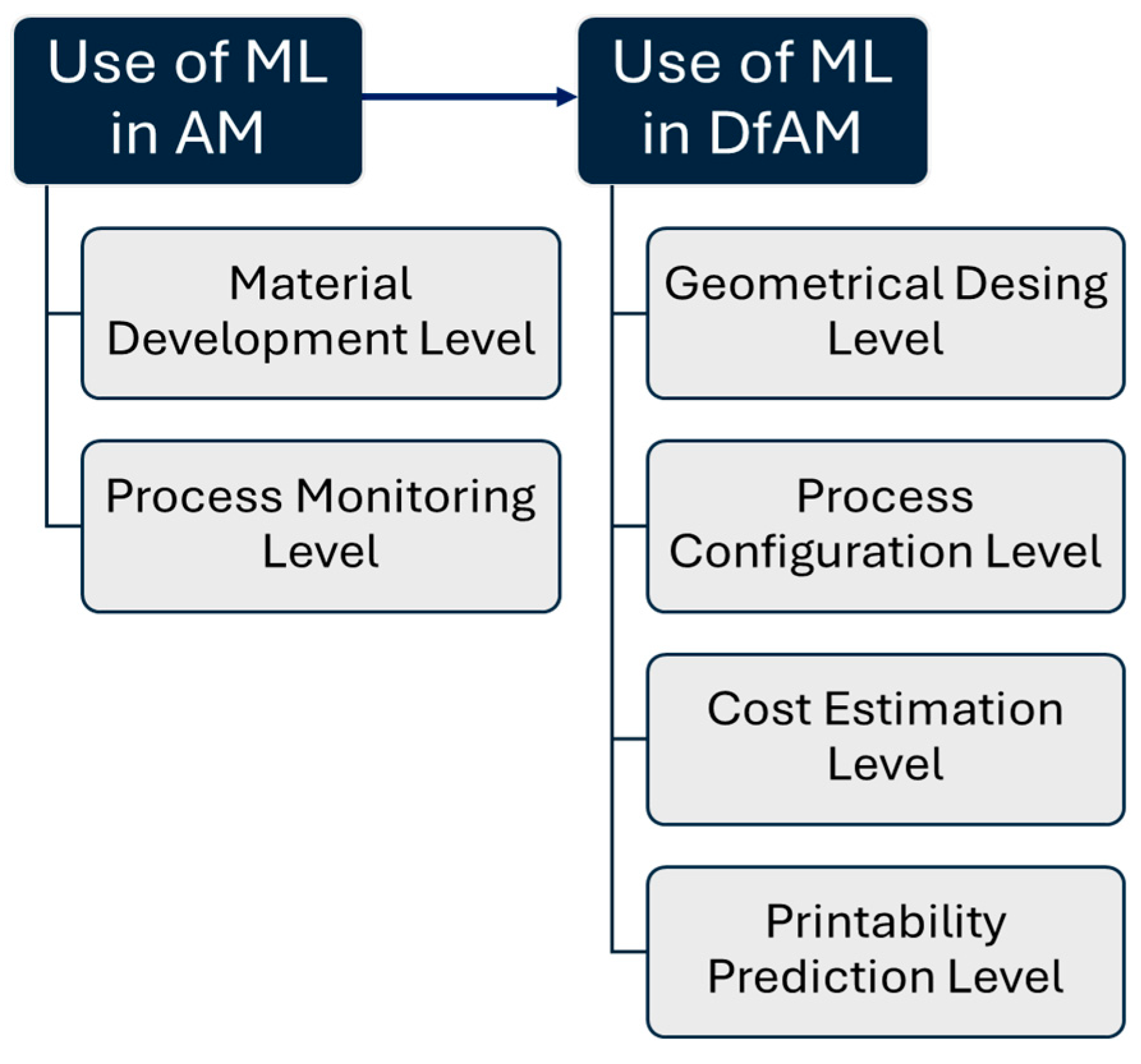
2.2. Machine Learning Applications in Design for Additive Manufacturing

The literature identifies numerous ML applications in the AM context. These applications can be divided into three levels: the Geometrical Design Level, the Process Configuration Level, and the Process Monitoring Level, also known as the “in situ” monitoring Level [34,35]. Other ML applications include cost estimation, material development, and printability prediction. Figure 3 shows this classification grouped in ML applications for AM and DfAM.

Starting from the ML usage in AM, two levels can be identified: the Material Development Level and the Process Monitoring Level. The first level involves the development of metal and composite materials using machine learning (ML) methods [36]. The second level, Process Monitoring, regards the real-time control of the printing process. SL algorithms are often used to classify and recognize issues during the printing phase. The possibility of checking the quality of the printed part during the process and modifying the process parameters to achieve better results makes this level relevant to the industrial world. Different methods, including image-based, optical-based, and acoustic-based techniques, are employed for monitoring the printing phase [37]. In [38], SVM and CNN are combined with a high-speed camera to control melt pool geometry, plume, and spatter, identifying issues during the printing phase. In [39], a hybrid ML model was trained on signals obtained from back reflection, visible, infrared, and structure-borne Acoustic Emission. The signals captured were used to classify the lack of fusion, conduction mode, and Keyhole. In [40], signals were acquired using a microphone, and acoustic signals were utilized for quality monitoring. Defect detection was achieved through the Deep Belief Network (DBN) framework.

Focusing on the use of ML in DfAM, these levels regard the phases of design, process configuration, cost estimation, and printability prediction.

The Geometrical Design Level concerns the methods for optimizing mass distribution in a component, including topology optimization (with SIMP and LSM algorithms) [41], Generative Design [42], and Lattice Structures [43], among others. There are also applications of ML methods in collaboration with classical optimization methods, where the potential of ML is leveraged to reduce the computational cost of optimization, thereby speeding up the process [44]. For example, in [45], a data-driven topology optimization model called TopologyGAN, where GAN is Generative Adversarial Networks, is proposed to bypass iterations and reduce computational costs. To optimize cells for a lattice structure [46], a GAN model is employed to generate Lattice Structures with a high strength-to-weight ratio.

The Process Configuration Level refers to the optimal values of the selected process parameters. The AM process parameters vary considerably depending on the technology, the material involved, the specific printer, and other factors. For example, for the L-PBF metal printing process, some of the main parameters for the printer setup include the spreading and granulometry of the powders, as well as laser power, scanning speed, hatch spacing, layer thickness, and laser beam size [47]. The high number of parameters and their value range make the introduction of ML systems helpful in selecting the parameters that yield the best results for the components in terms of mechanical properties, surface roughness, and other relevant factors. To improve the spreading parameters, for example, a Back Propagation Neural Network with one hidden layer was used [48] to optimize the final Roughness and porosity of a part. In [49], an SVM, supported by X-ray microtomography, was trained to identify relationships between fatigue life and the size, location, and morphology of defects. In [50], an ANN, an RF, and an SVM were trained and compared for predicting fatigue life from process parameters such as laser power, scan speed, hatch space, and powder layer thickness.

The Cost Estimation Level predicts the cost of printing a part. Typically, the approaches for calculating costs are analytical and involve calculating material cost, machine cost, operator cost, and costs related to energy consumption, maintenance, and administration, among others. ML approaches can also support this phase. For example, in [51], a cost-analytic framework has been developed, utilizing the extracted data features from CAD models. These features were built using a dynamic clustering method based on the k-means algorithm for variance reduction, and regression models were employed for cost prediction.

The Printability Prediction Level is a powerful tool that enhances the AM process by forecasting potential issues, guiding design improvements, and ultimately leading to the more successful and efficient production of complex parts. Reducing issues related to printability is the primary way to reduce printing costs, as it is often impossible to reduce the costs of raw materials and equipment. In [52], a framework was developed to predict printability, detailing a method for measuring small-scale printability even on complex components containing large-scale defects. In [53], a study was released to predict the dimensional deviations of manufactured objects. The input to the error prediction ANN is information extracted from the model’s mesh to be manufactured. The output of the ANN is the estimated average per vertex error for the fabricated object. In [54], a Decision Tree approach was trained to predict the printability of metal components, starting from geometrical features extracted from the CAD model and using L-PBF process simulations.

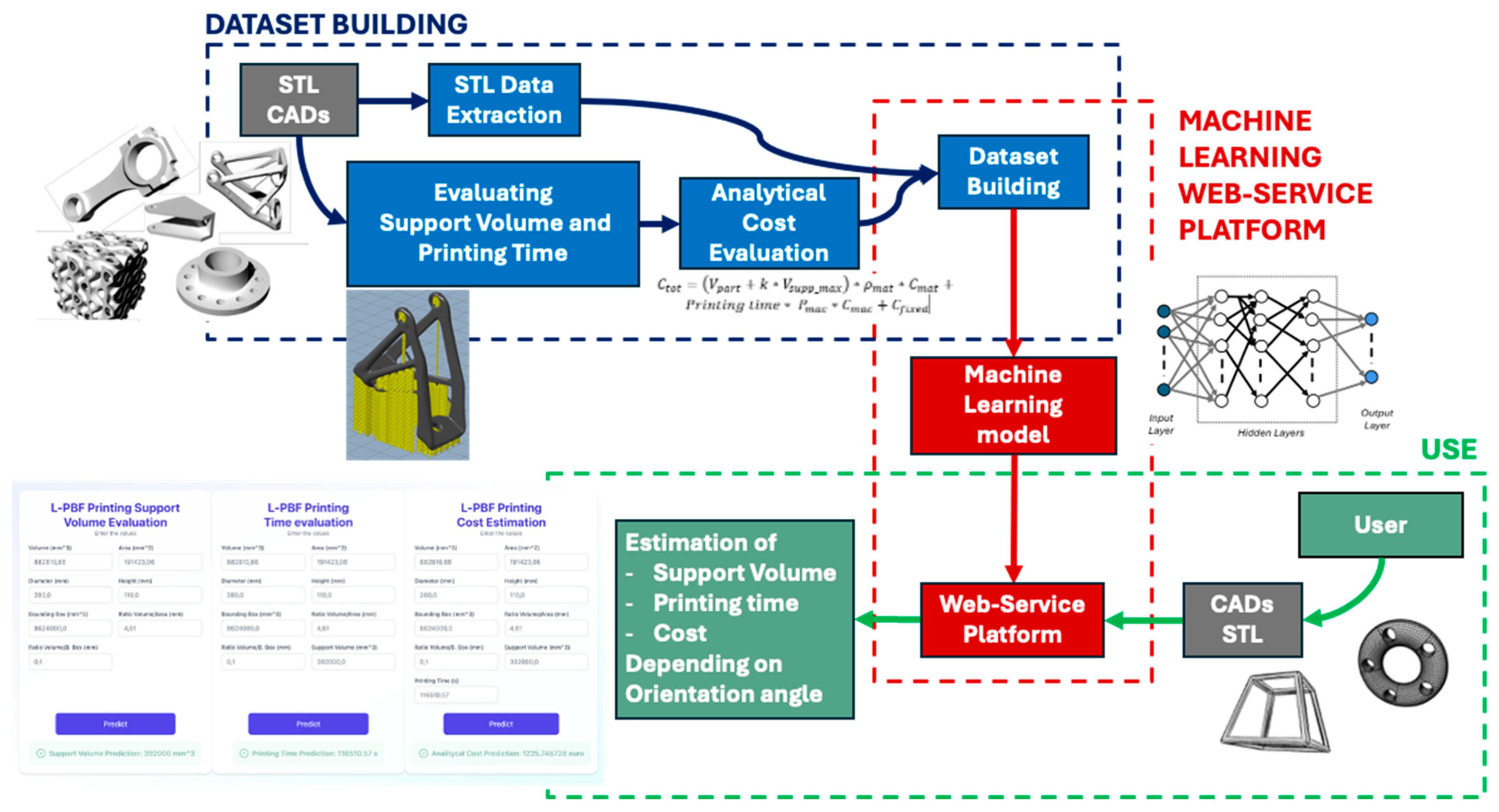
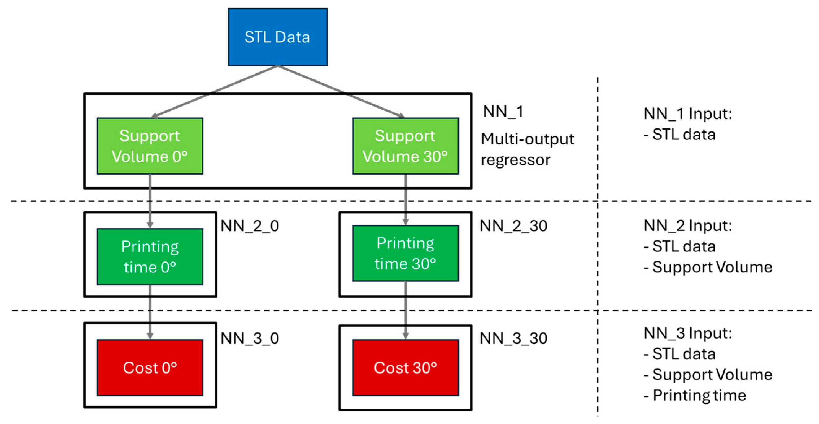
3. Proposed Approach

The objective of this paper is to develop an ML-based web service platform that supports engineers in assessing Support Volume, 3D Printing Time, and Cost of metal parts realized by L-PBF. Figure 4 illustrates the proposed approach, highlighting three phases: Dataset Building, Machine Learning Web-Service Platform, and Use.

The first phase involves implementing the dataset through CAD models and virtual experiments. Physical prototypes can also be created, if possible, to reduce uncertainties resulting from software calculations. A code automatically extracts features from the geometry to acquire the necessary input data. The STL format was used for the CAD files.

This file format describes a three-dimensional model by splitting up its surfaces into numerous triangle facets that together characterize the geometry and contour of the object. At this point, the target values for Support Volume, 3D Printing Time, and Cost are evaluated. While Support Volume and 3D Printing Time are evaluated using simulation software, the cost is analyzed through an analytical approach. Equation (1) reports the formula used for the cost evaluation:

$$C_{tot}=\left(V_{part}+k\ast V_{supp\_max}\right)\ast {\rho }_{mat}\ast C_{mat}+Printingtime\ast {\overline{P}}_{mac}\ast C_{mac}+C_{fixed}$$

(1)

where $C_{tot}$ is the total cost evaluated in €, $V_{part}$ is the volume of the part to be printed (mm³), k (dimensionless) is the ratio between the effective and maximum volume support $V_{supp\_max}$ (mm³), and its value varies between 0 and 1, depending on the type of support structure used; the most common are lattice and block support structures [55] (typical values for k: 0.2–0.5), ${\rho }_{mat}$ is the material density (kg/mm³), $C_{mat}$ is the material cost (€/kg), ${\overline{P}}_{mac}$ is the average machine power (kW), and $C_{mac}$ is the specific energy cost (€/kWh), and $C_{fixed}$ is the fixed cost, such as machine depreciation, scheduled maintenance, human-related cost, etc. The scope of the methodology is restricted to the 3D printing process as it is, without considering post-processing or machining, therefore considering only net-shape components optimal for AM production.

The second phase, related to the development of the web service, can be divided into two levels: defining the ML model and the development of the web service platform, which is the Model Endpoint. The first level concerns the training and testing of the ML model to predict Support Volume, 3D Printing Time, and Cost related to a CAD model to be printed. On the other hand, the second level regards the implementation of a web service platform that exploits the trained ML models inside an online system designed to streamline and support the technical users.

The use phase describes the workflow of input/output provided by the analyzed web platform to predict the time and cost for a CAD model to be realized by L-PBF.

4. Case Study

This case study describes the application of the proposed method to support the DfAM of Ti-6Al-4V flanges. The implemented ML system predicts the 3D Printing Time and printing cost of these components by analyzing the specific geometrical features. The analyzed parts were designed to be realized by L-PBF. The 3D printer used for reference is the EOS M400-4. This printer has a build volume of 400 × 400 × 400 mm, four 400 W fiber lasers, and a mean power consumption of 22 kW.

The ML training is based on virtual experiments. The CAD models employed were generated using a CAD automation tool that integrates VB.NET code with Autodesk Inventor^® (https://www.autodesk.com/), using a CAD model template with geometrical parameters. These parameters regard diameters, thicknesses, the number of holes, height, and others.

A total of 235 CAD models (dataset samples) of parametric flanges have been produced using a DOE table of parameter combinations. Each CAD model was exported in STL format (Figure 5a). To generate the dataset labels and targets were extracted and calculated from the CAD models. The extracted labels regard the geometrical features acquired by a Python 3.11 code. The Python code uses the open-source library “numpy-stl 3.2.0” [56]. From this analysis, the following parameters were considered geometrical labels: Volume, Area, Diameter, Height, Bounding box, Ratio Volume/Area, and Ratio Volume/Bounding Box. Support Volume, 3D Printing Time, and Cost have been considered as targets. Diameter and Height are calculated from the Bounding Box dimension extracted using the library; they are related only to this test case geometry. For more complex geometries, the features will be extracted accordingly from CAD models.

While Support Volume and 3D Printing Time have been obtained by performing 3D printing analysis with Altair^® Inspire^TM (Figure 5b), the Cost label has been calculated using Equation (1). Fixed costs have not been included in this case study, being a constant of AM processes, depending case by case on the company procedures. The case study considers only the $C_{AM}$. For the final cost evaluation, post-processing, such as thermal treatment and finishing surfaces, must be considered. This test case focuses only on $C_{AM}$.

Considering the possibility of different part orientations, the dataset was built into two subsets: one considering 0° of part orientation on the 3D printing plate and one considering 30° of part orientation. The 0° orientation refers to the solution that minimizes the 3D Printing Time, and the 30° solution comes from the experience of simulations to lower residual stresses and deformations. The plate distance has always been considered 5 mm for the dataset realization. Therefore, two parallel ML models were trained using NNs.

Figure 6 illustrates the overall prediction model, which is divided into two channels (0° and 30°). Each channel consists of three NNs. Using three NNs for each channel instead of a single one allows the output of the first NN to be used as input for the second and the output of the second to be used as input for the third.

Support Volume is predicted as a target in the first NN and used as a label in the second NN to predict 3D Printing Time. Similarly, Support Volume and 3D Printing Time are used as labels to predict the Cost in the third NN. With the data automatically extracted from the STL CAD models (geometrical labels), the first NN, called NN_1, has been trained to obtain the Support Volume at 0° and 30° using the multi-output regressor technique. NN_2_0 and NN_2_30 use labels referring to the orientation of the study. NN_2_0 uses the geometrical labels and the “Support Volume 0°” to predict the 3D Printing Time. In the same manner, NN_3_0 and NN_3_30 are trained to predict the Cost of the 3D printing part using STL data, support volume, and printing time as labels. All the trained NNs use the same hyperparameters, described in

Table 3. Hyperparameters used to train NNs.

Hyperparameter	Value/Type
Hidden layers	5
Neuron per hidden layer	25, 50, 100, 50, 25
Activation function	ReLU
Solver	Adam
Maximum iteration	1000

. The dataset has been divided into train and test samples, with a test size of 20%.

When dealing with a pipeline of NNs, it is important to consider the error propagation from earlier predictions to later ones. Understanding and managing error propagation is crucial in any pipeline, where predictions feed into future ones. Without mitigation, even small early mistakes can lead to significant degradation in performance, reducing the reliability of the entire system. For example, in this case, errors in Support Volume predictions can directly impact the inputs of Printing Time in the same manner as Printing Time on Cost predictions.

The dataset normalization allows the comparison of variables that have means and standard deviations measured on different units of measurement and orders of magnitude. In this paper, the open-source library “StandardScaler” [57]. Three different metrics have been adopted to evaluate and compare training and testing results such as the Mean Squared Error (MSE), the Mean Absolute Error (MAE), and R² (coefficient of determination).

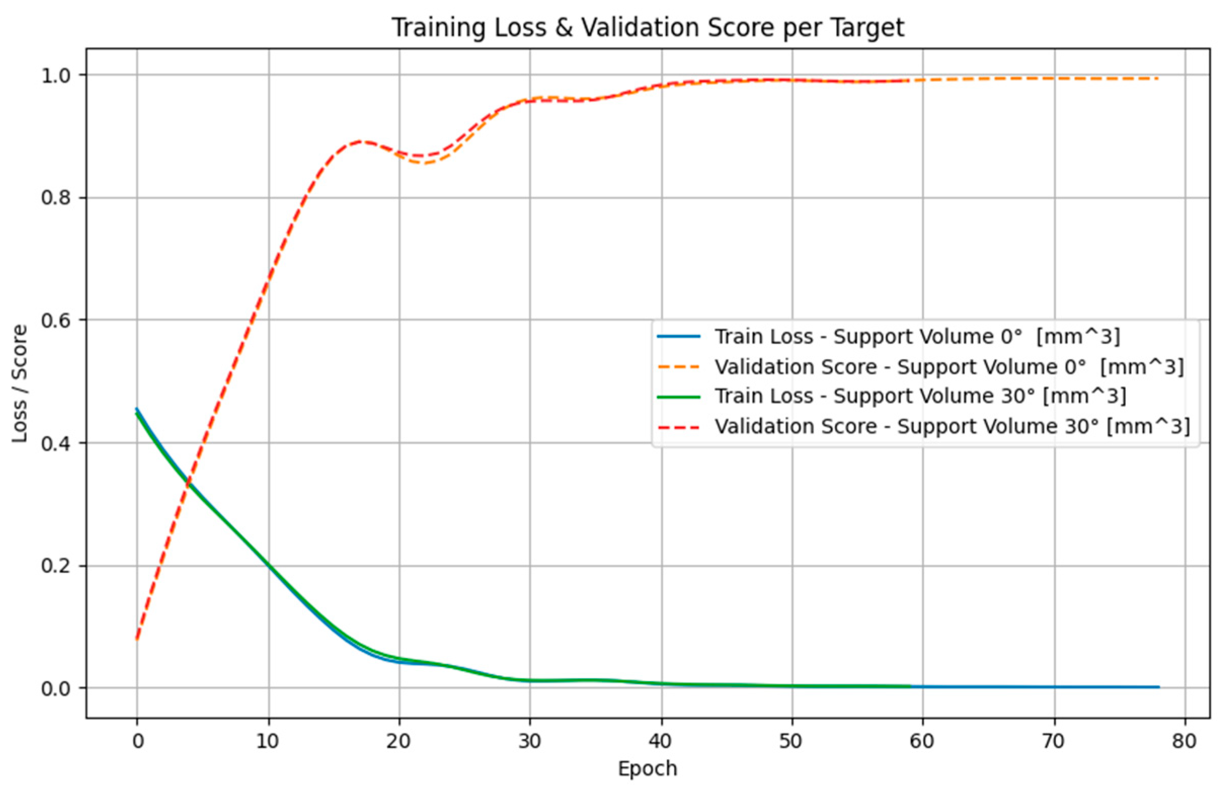
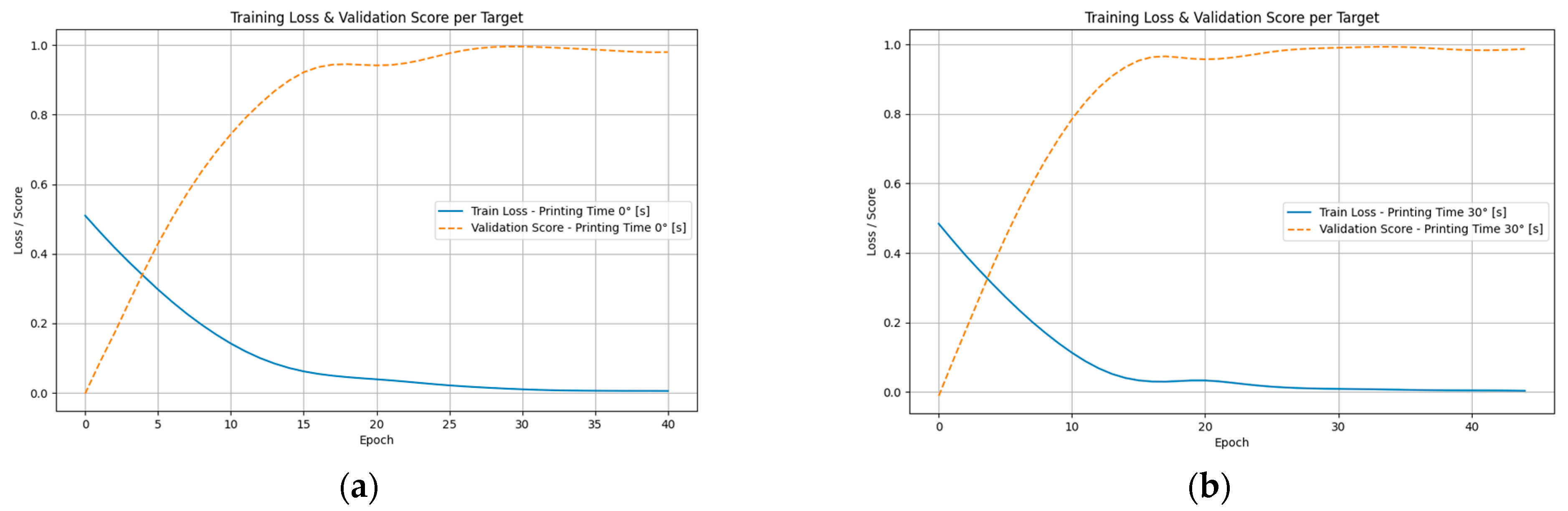
4.1. Training Results

Table 4. Performance metrics of the NN_1 model.

NN_1	Train Metrics	Test Metrics
Support Volume 0°	R2: 0.9975	R2: 0.9973
	MSE: 0.0022	MSE: 0.0037
	MAE: 0.0338	MAE: 0.0416
Support Volume 30°	R2: 0.9930	R2: 0.9912
	MSE: 0.0062	MSE: 0.0125
	MAE: 0.0602	MAE: 0.0704

,

Table 5. Performance metrics of the NN_2_0 and NN_2_30 models.

NN_2	Train Metrics	Test Metrics
NN_2_0: Printing Time 0°	R2: 0.9799	R2: 0.9864
	MSE: 0.0191	MSE: 0.0163
	MAE: 0.0992	MAE: 0.1036
NN_2_30: Printing Time 30°	R2: 0.9865	R2: 0. 9846
	MSE: 0.0122	MSE: 0.0212
	MAE: 0.0811	MAE: 0.1023

and

Table 6. Performance metrics of the NN_3_0 and NN_3_30 models.

NN_3	Train Metrics	Test Metrics
NN_3_0: Analytical Cost 0°	R2: 0.9984	R2: 0.9965
	MSE: 0.0015	MSE: 0.0044
	MAE: 0.0284	MAE: 0.0457
NN_3_30: Analytical Cost 30°	R2: 0.9983	R2: 0.9937
	MSE: 0.0015	MSE: 0.0044
	MAE: 0.0295	MAE: 0.0527

list the metrics obtained to evaluate the NN models, such as MSE, MAE, and R², for the train and test phases. Each metric evaluates a specific aspect of the trained model. Low MSE values imply that the model’s predictions are close to the target values. MAE values measure the average amplitude of errors without considering their sign. The R² value indicates how well the model’s predictions match the data. R² values vary from 0 to 1, with 1 representing perfect prediction and 0 indicating no predictive power. Figure 7, Figure 8 and Figure 9 show the convergence trend, and thus the Loss trend and Validation score at each epoch for the trained NN. The Loss function measures the difference between the network’s prediction and the actual target value using the MSE metric for regression problems. At each epoch, the prediction and the relative loss function are computed, gradients are computed using the chain rule, and the weights are updated, leading to new predictions and a new loss until convergence or early stopping.

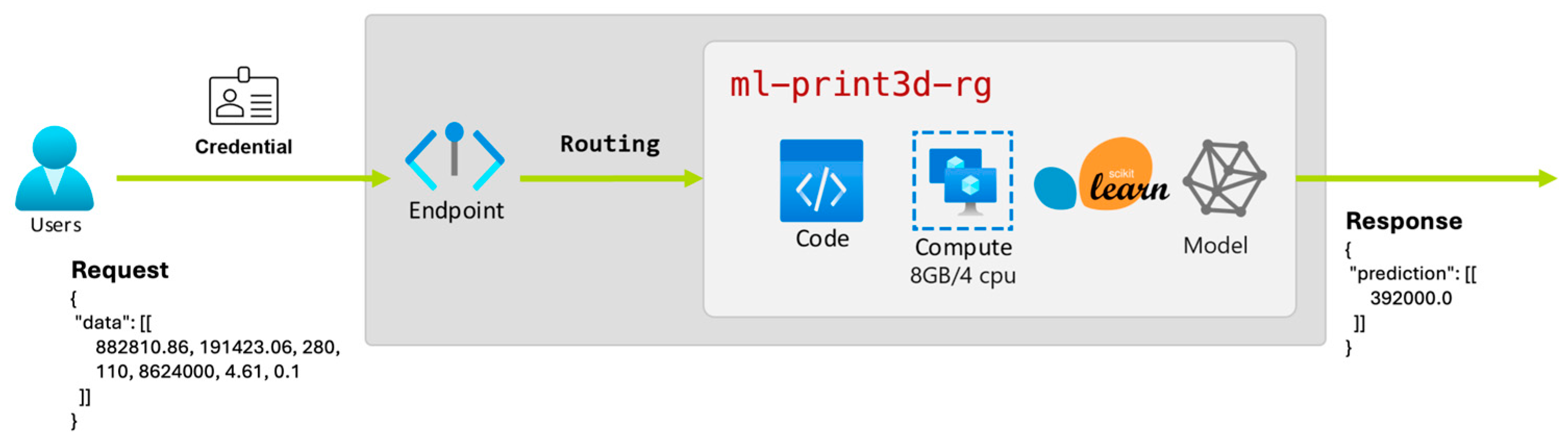
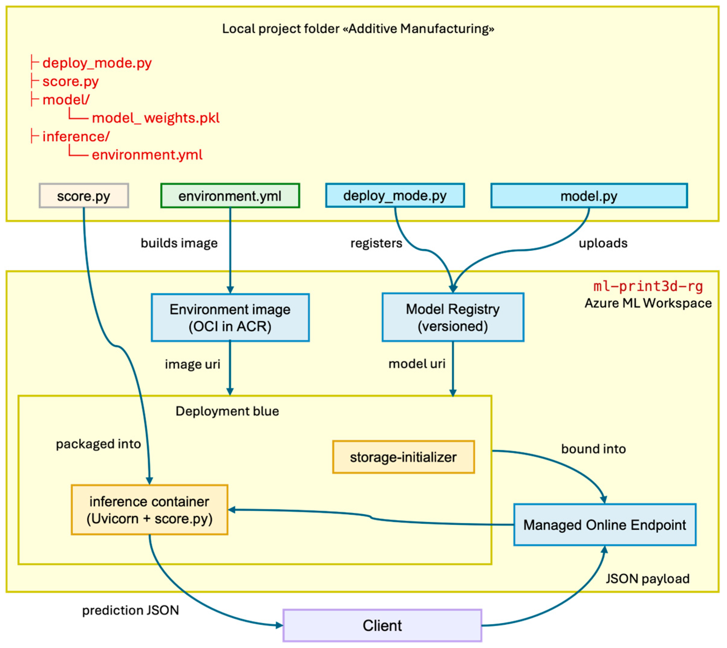
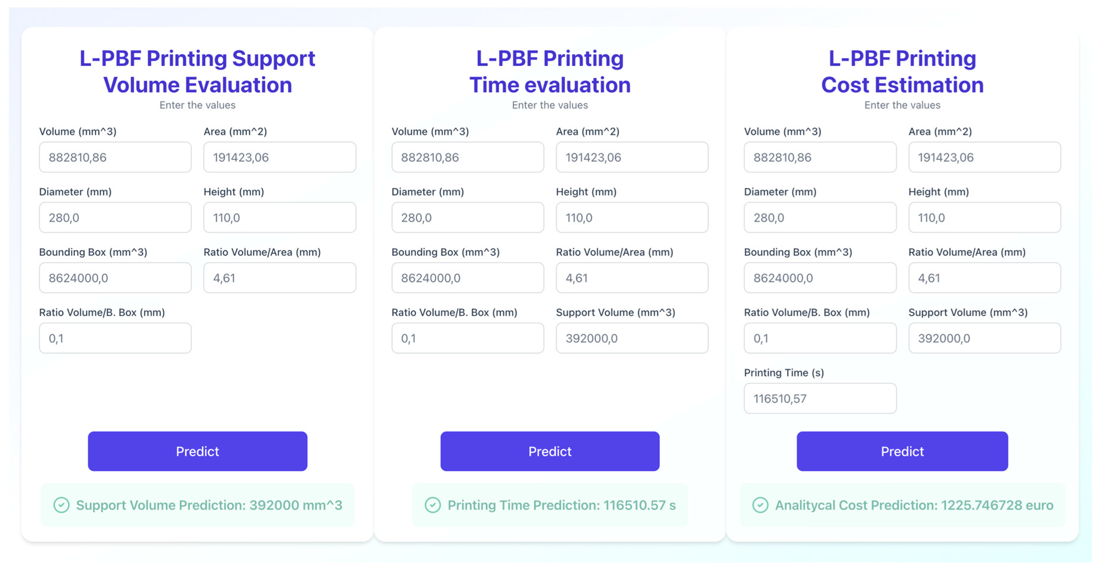
4.2. Web-Service Platform Development

An endpoint is a network-exposed interface that delivers a trained model’s inference function as a stateless web service and deploys the model as a cloud-hosted endpoint. This approach, compared to local instances, ensures reproducible access, scalable computation, centralized monitoring, and seamless integration into diverse research workflows.

ML practical implications in operational settings are generally based on specific tools available on the market. In this section, the realization of an endpoint service using the commercial tool Microsoft AzureML [58] is introduced. Figure 10 presents the architecture of the client-to-cloud inference pathway, in which end-users interact with a Machine-Learning endpoint as a managed HTTPS service.

The user initiates the transaction by attaching an authentication credential to an HTTP POST request, whose body contains labeled data in a JSON object, as required by the deployed model. Upon receipt, the endpoint (Figure 11) computes the output, makes the prediction, and re-formulates the named prediction in a JSON structure, returning synchronously to the client through the same channel.

In particular, when the message reaches the endpoint, a gateway service performs input validation and executes routing logic. In the experimental scenario, 100% of traffic is forwarded to ml-print3d-rg, where there are four encapsulated layers:

• Code: the score.py script that implements init() (model loading) and run() (prediction).
• Compute: a dedicated container instance with 8 GB RAM and 4 vCPU, provisioned from the Stock Keeping Unit (SKU) selected during deployment creation.
• Scikit-learn runtime: the framework layer installed via the Azure ML Environment image.
• Model: the serialized estimator, which resides in the container’s mounted storage and is loaded into memory at start-up.

The practical realization of this workflow is captured in a self-contained repository. Its structure mirrors the logical artifacts described in Figure 12. The workflow is based on the deploy_mode.py file; a Python code that authenticates to the Azure ML workspace and registers the serialized model; and Conda environment that provisions a Managed Online Endpoint, instantiates a first deployment (blue) on an appropriate Virtual Machine SKU, and directs 100% of traffic to that deployment. Within a model/ directory, there is a model_weights.pkl that embodies the trained estimator weights, enabling strict versioning in the Model Registry thanks to its immutability.

The inference/ folder contains two artifacts that together define the run-time surface of the service: score.py file, which implements the init() routine for loading the pickle, and the run() routine that transforms incoming JSON payloads feature matrices before invoking model.predict(), and environment.yml, a declarative Conda specification whose pip section includes azureml-inference-server-http, thereby ensuring that Azure ML can synthesize a fully compatible OCI image (container image). By coupling these code modules with the platform objects (workspace, registry, endpoint, and deployment), the repository serves as an executable blueprint that allows any practitioner to replicate the end-to-end process, elevating a research-grade model to a production-grade online endpoint.

The results of an HTTP POST request are shown in Figure 13, where a browser-based inference interface is highlighted. Each card is dedicated to a specific predictive task within the L-PBF process planning.

5. Discussion and Conclusions

The research scope is the study of an applicative method to develop an ML-based web service platform that supports engineers in defining geometries to be realized by L-PBF. The paper proposes a Neural Network approach to evaluate data such as Support Volume, 3D Printing Time, and Cost, implementing the resulting model in a Web-Service Platform secured by a login system. The ML model consists of an NN pipeline with three regression steps. The input data concerns geometrical features extracted directly from STL files. The approach can be applied universally; however, the test case focuses on the design of metallic flanges. The training phase was conducted using a dataset of 235 randomly generated samples from a CAD template model. The results show high R² values greater than 0.97. The pipeline was implemented into a commercial web service and tested with authorized users to emulate a production-grade online endpoint.

In this paper, the methodology is presented through a simplified case study, adopted as a proof of concept to support the implementation of ML in DfAM. As analyzed, ML enhances the capabilities of AM processes, improving geometry optimization, material efficiency, process parameter selection and ensuring high quality through real-time monitoring and predictive maintenance. For future instances, the study will be extended to include various geometries, printing orientations, and materials. However, considering different types of parts, new training and testing phases are necessary to provide a more general model.

References

1. Bonnard, R.; Hascoët, J.-Y.; Mognol, P.; Zancul, E.; Alvares, A.J. Hierarchical object-oriented model (HOOM) for additive manufacturing digital thread. J. Manuf. Syst. 2019, 50, 36–52. [Google Scholar] [CrossRef]
2. Dilberoglu, U.M.; Gharehpapagh, B.; Yaman, U.; Dolen, M. The Role of Additive Manufacturing in the Era of Industry 4.0. Procedia Manuf. 2017, 11, 545–554. [Google Scholar] [CrossRef]
3. Mies, D.; Marsden, W.; Warde, S. Overview of Additive Manufacturing Informatics: “A Digital Thread”. Integr. Mater. Manuf. Innov. 2016, 5, 114–142. [Google Scholar] [CrossRef]
4. ISO/ASTM 52900:2021; Additive Manufacturing—General Principles—Fundamentals and Vocabulary. ISO/ASTM International: Geneva, Switzerland, 2021.
5. Shi, Y.; Zhang, Y.; Baek, S.; De Backer, W.; Harik, R. Manufacturability analysis for additive manufacturing using a novel feature recognition technique. Comput.-Aided Des. Appl. 2018, 15, 941–952. [Google Scholar] [CrossRef]
6. Haines, M.P.; Peter, N.J.; Babu, S.S.; Jägle, E.A. In-situ synthesis of oxides by reactive process atmospheres during L-PBF of stainless steel. Addit. Manuf. 2020, 33, 101178. [Google Scholar] [CrossRef]
7. Vaneker, T.; Bernard, A.; Moroni, G.; Gibson, I.; Zhang, Y. Design for additive manufacturing: Framework and methodology. CIRP Ann. 2020, 69, 578–599. [Google Scholar] [CrossRef]
8. Lynn, R.; Saldana, C.; Kurfess, T.; Reddy, N.; Simpson, T.; Jablokow, K.; Tucker, T.; Tedia, S.; Williams, C. Toward Rapid Manufacturability Analysis Tools for Engineering Design Education. Procedia Manuf. 2016, 5, 1183–1196. [Google Scholar] [CrossRef]
9. Trovato, M.; Cicconi, P. Design tools for metal additive manufacturing: A critical and perspective overview. Procedia CIRP 2023, 119, 1084–1090. [Google Scholar] [CrossRef]
10. Kaščák, Ľ.; Varga, J.; Bidulská, J.; Bidulský, R.; Manfredi, D. Weight Factor as a Parameter for Optimal Part Orientation in the L-PBF Printing Process Using Numerical Simulation. Materials 2024, 17, 3604. [Google Scholar] [CrossRef]
11. Dixit, S.; Liu, S.; Murdoch, H.A.; Smith, P.M. Investigating build orientation-induced mechanical anisotropy in additive manufacturing 316L stainless steel. Mater. Sci. Eng. A 2023, 880, 145308. [Google Scholar] [CrossRef]
12. Bianchi, I.; Forcellese, A.; Forcellese, P.; Mancia, T.; Mignanelli, C.; Simoncini, M.; Verdini, T. Effect of Printing Orientation Angle and Heat Treatment on the Mechanical Properties and Microstructure of Binder-Jetting-Printed Parts in 17-4 PH Stainless Steel. Metals 2024, 14, 1220. [Google Scholar] [CrossRef]
13. Rabalo, M.A.; Rubio, E.M.; Agustina, B.; Camacho, A.M. Hybrid additive and subtractive manufacturing: Evolution of the concept and last trends in research and industry. Procedia CIRP 2023, 118, 741–746. [Google Scholar] [CrossRef]
14. Schmitz, T.; Corson, G.; Olvera, D.; Tyler, C.; Smith, S. A framework for hybrid manufacturing cost minimization and preform design. CIRP Ann. 2023, 72, 373–376. [Google Scholar] [CrossRef]
15. Sharifani, K.; Amini, M. Machine Learning and Deep Learning: A Review of Methods and Applications. World Inf. Technol. Eng. J. 2023, 10, 3897–3904. [Google Scholar]
16. Jiang, Y.; Li, X.; Luo, H.; Yin, S.; Kaynak, O. Quo vadis artificial intelligence? Discov. Artif. Intell. 2022, 2, 4. [Google Scholar] [CrossRef]
17. Mahesh, B. Machine Learning Algorithms—A Review. Int. J. Sci. Res. 2020, 9, 381–386. [Google Scholar] [CrossRef]
18. Cunningham, P.; Cord, M.; Delany, S.J. Supervised Learning. In Machine Learning Techniques for Multimedia: Case Studies on Organization and Retrieval; Springer: Berlin/Heidelberg, Germany, 2008; pp. 21–49. [Google Scholar]
19. Dayan, P. Unsupervised Learning. In The MIT Encyclopedia of the Cognitive Sciences; Wilson, R.A., Keil, F., Eds.; MIT Press: Cambridge, MA, USA, 2001. [Google Scholar]
20. Luo, F.M.; Xu, T.; Lai, H.; Chen, X.H.; Zhang, W.; Yu, Y. A survey on model-based reinforcement learning. Sci. China Inf. Sci. 2024, 67, 121101. [Google Scholar] [CrossRef]
21. Joshi, M.; Flood, A.; Sparks, T.; Liou, F.W. Applications of supervised machine learning algorithms in additive manufacturing: A review. In 2019 International Solid Freeform Fabrication Symposium; University of Texas at Austin: Austin, TX, USA, 2019. [Google Scholar]
22. Zhang, Y.; Safdar, M.; Xie, J.; Li, J.; Sage, M.; Zhao, Y.F. A systematic review on data of additive manufacturing for machine learning applications: The data quality, type, preprocessing, and management. J. Intell. Manuf. 2022, 34, 3305–3340. [Google Scholar] [CrossRef]
23. García-Moreno, A.-I.; Alvarado-Orozco, J.-M.; Ibarra-Medina, J.; Martínez-Franco, E. Image-based porosity classification in Al-alloys by laser metal deposition using random forests. Int. J. Adv. Manuf. Technol. 2020, 110, 2827–2845. [Google Scholar] [CrossRef]
24. Kumar, P.; Jain, N.K. Surface roughness prediction in micro-plasma transferred arc metal additive manufacturing process using K-nearest neighbors algorithm. Int. J. Adv. Manuf. Technol. 2022, 119, 2985–2997. [Google Scholar] [CrossRef]
25. Vandecasteele, M.; Heylen, R.; Iuso, D.; Thanki, A.; Philips, W.; Witvrouw, A.; Verhees, D.; Booth, B.G. Towards material and process agnostic features for the classification of pore types in metal additive manufacturing. Mater. Des. 2023, 227, 111757. [Google Scholar] [CrossRef]
26. Banadaki, Y.M.; Razaviarab, N.; Fekrmandi, H.; Li, G.; Mensah, P.; Bai, S.; Sharifi, S. Automated Quality and Process Control for Additive Manufacturing using Deep Convolutional Neural Networks. Recent Prog. Mater. 2021, 4, 5. [Google Scholar] [CrossRef]
27. Xiao, S.; Li, J.; Wang, Z.; Chen, Y.; Tofighi, S. Advancing Additive Manufacturing Through Machine Learning Techniques: A State-of-the-Art Review. Future Internet 2024, 16, 419. [Google Scholar] [CrossRef]
28. Baturynska, I.; Semeniuta, O.; Martinsen, K. Optimization of Process Parameters for Powder Bed Fusion Additive Manufacturing by Combination of Machine Learning and Finite Element Method: A Conceptual Framework. Procedia CIRP 2018, 67, 227–232. [Google Scholar] [CrossRef]
29. Mattera, G.; Piscopo, G.; Longobardi, M.; Giacalone, M.; Nele, L. Improving the Interpretability of Data-Driven Models for Additive Manufacturing Processes Using Clusterwise Regression. Mathematics 2024, 12, 2559. [Google Scholar] [CrossRef]
30. Song, L.; Huang, W.; Han, X.; Mazumder, J. Real-Time Composition Monitoring Using Support Vector Regression of Laser-Induced Plasma for Laser Additive Manufacturing. IEEE Trans. Ind. Electron. 2017, 64, 633–642. [Google Scholar] [CrossRef]
31. Zhu, X.; Jiang, F.; Guo, C.; Wang, Z.; Dong, T.; Li, H. Prediction of melt pool shape in additive manufacturing based on machine learning methods. Opt. Laser Technol. 2023, 159, 108964. [Google Scholar] [CrossRef]
32. Equbal, M.A.; Equbal, A.; Khan, Z.A.; Badruddin, I.A. Machine learning in Additive Manufacturing: A Comprehensive insight. Int. J. Lightweight Mater. Manuf. 2025, 8, 264. [Google Scholar] [CrossRef]
33. Ciccone, F.; Bacciaglia, A.; Ceruti, A. Optimization with artificial intelligence in additive manufacturing: A systematic review. J. Braz. Soc. Mech. Sci. Eng. 2023, 45, 303. [Google Scholar] [CrossRef]
34. Trovato, M.; Belluomo, L.; Bici, M.; Prist, M.; Campana, F.; Cicconi, P. Machine learning in design for additive manufacturing: A state-of-the-art discussion for a support tool in product design lifecycle. Int. J. Adv. Manuf. Technol. 2025, 137, 2157–2180. [Google Scholar] [CrossRef]
35. Trovato, M.; Belluomo, L.; Bici, M.; Campana, F.; Cicconi, P. Machine Learning Trends in Design for Additive Manufacturing. In Design Tools and Methods in Industrial Engineering III; Lecture Notes in Mechanical Engineering; Springer: Cham, Switzerland, 2024; pp. 109–117. [Google Scholar]
36. Johnson, N.S.; Vulimiri, P.S.; To, A.C.; Zhang, X.; Brice, C.A.; Kappes, B.B.; Stebner, A.P. Invited review: Machine learning for materials developments in metals additive manufacturing. Addit. Manuf. 2020, 36, 101641. [Google Scholar] [CrossRef]
37. Jin, Z.; Zhang, Z.; Demir, K.; Gu, G.X. Machine Learning for Advanced Additive Manufacturing. Matter 2020, 3, 1541–1556. [Google Scholar] [CrossRef]
38. Zhang, Y.; Hong, G.S.; Ye, D.; Zhu, K.; Fuh, J.Y.H. Extraction and evaluation of melt pool, plume and spatter information for powder-bed fusion AM process monitoring. Mater. Des. 2018, 156, 458–469. [Google Scholar] [CrossRef]
39. Pandiyan, V.; Masinelli, G.; Claire, N.; Le-Quang, T.; Hamidi-Nasab, M.; de Formanoir, C.; Esmaeilzadeh, R.; Goel, S.; Marone, F.; Logé, R.; et al. Deep learning-based monitoring of laser powder bed fusion process on variable time-scales using heterogeneous sensing and operando X-ray radiography guidance. Addit. Manuf. 2022, 58, 103007. [Google Scholar]
40. Ye, D.; Hong, G.S.; Zhang, Y.; Zhu, K.; Fuh, J.Y.H. Defect detection in selective laser melting technology by acoustic signals with deep belief networks. Int. J. Adv. Manuf. Technol. 2018, 96, 2791–2801. [Google Scholar] [CrossRef]
41. Sigmund, O.; Maute, K. Topology optimization approaches. Struct. Multidiscip. Optim. 2013, 48, 1031–1055. [Google Scholar] [CrossRef]
42. Krish, S. A practical generative design method. Comput.-Aided Des. 2011, 43, 88–100. [Google Scholar] [CrossRef]
43. Amicarelli, M.; Trovato, M.; Cicconi, P. Lightweight Design of a Connecting Rod Using Lattice-Structure Parameter Optimisations: A Test Case for L-PBF. Machines 2025, 13, 171. [Google Scholar] [CrossRef]
44. Hsiao, S.-W.; Tsai, H.-C. Applying a hybrid approach based on fuzzy neural network and genetic algorithm to product form design. Int. J. Ind. Ergon. 2005, 35, 411–428. [Google Scholar] [CrossRef]
45. Nie, Z.; Lin, T.; Jiang, H.; Kara, L.B. TopologyGAN: Topology Optimization Using Generative Adversarial Networks Based on Physical Fields Over the Initial Domain. J. Mech. Des. 2021, 143, 031715. [Google Scholar] [CrossRef]
46. Yüksel, N.; Eren, O.; Börklü, H.R.; Sezer, H.K. Mechanical properties of additively manufactured lattice structures designed by deep learning. Thin-Walled Struct. 2024, 196, 111475. [Google Scholar] [CrossRef]
47. Uriati, F.; Nicoletto, G. A comparison of Inconel 718 obtained with three L-PBF production systems in terms of process parameters, as-built surface quality, and fatigue performance. Int. J. Fatigue 2022, 162, 107004. [Google Scholar] [CrossRef]
48. Zhang, W.; Mehta, A.; Desai, P.S.; Higgs III, C.F. Machine learning enabled powder spreading process map for metal additive manufacturing (AM). In Proceedings of the 2018 Annual International Solid Freeform Fabrication Symposium—An Additive Manufacturing Conference, Austin, TX, USA, 13–15 August 2018. [Google Scholar]
49. Bao, H.; Wu, S.; Wu, Z.; Kang, G.; Peng, X.; Withers, P.J. A machine-learning fatigue life prediction approach of additively manufactured metals. Eng. Fract. Mech. 2021, 242, 107508. [Google Scholar] [CrossRef]
50. Zhan, Z.; Li, H. Machine learning based fatigue life prediction with effects of additive manufacturing process parameters for printed SS 316L. Int. J. Fatigue 2021, 142, 105941. [Google Scholar] [CrossRef]
51. Chan, S.L.; Lu, Y.; Wang, Y. Data-driven cost estimation for additive manufacturing in cybermanufacturing. J. Manuf. Syst. 2018, 46, 115–126. [Google Scholar] [CrossRef]
52. Mycroft, W.; Katzman, M.; Tammas-Williams, S.; Hernandez-Nava, E.; Panoutsos, G.; Todd, I.; Kadirkamanathan, V. A data-driven approach for predicting printability in metal additive manufacturing processes. J. Intell. Manuf. 2020, 31, 1769–1781. [Google Scholar] [CrossRef]
53. Ntousia, M.; Fudos, I.; Moschopoulos, S.; Stamati, V. Predicting geometric errors and failures in additive manufacturing. Rapid Prototyp. J. 2023, 29, 1843–1861. [Google Scholar] [CrossRef]
54. Trovato, M.; Cicconi, P. A Decision Tree approach for an early evaluation of 3D models in Design for Additive Manufacturing. Procedia CIRP 2024, 128, 96–101. [Google Scholar] [CrossRef]
55. Su, J.; Mo, Y.; Shangguan, P.; Panwisawas, C.; Jiang, F.; Sing, S.L. Additive manufacturing-by-design for support structures: A critical review. Int. J. Extrem. Manuf. 2025, 7, 052002. [Google Scholar] [CrossRef]
56. numpy-stl 3.2.0. PyPI—Python Package Index. Available online: https://pypi.org/project/numpy-stl/ (accessed on 11 May 2025).
57. StandardScaler. Scikit-Learn Documentation. Available online: https://scikit-learn.org/stable/modules/generated/sklearn.preprocessing.StandardScaler.html# (accessed on 11 May 2025).
58. Azure Machine Learning. Microsoft Learn. Available online: https://learn.microsoft.com/en-us/azure/machine-learning/?view=azureml-api-2 (accessed on 11 May 2025).
Figure 1. Machine learning classification scheme.
Machines 13 00550 g001
Figure 2. Cyclical workflow to implement ML in industrial production.
Machines 13 00550 g002
Figure 3. The different application levels of ML techniques in AM and DfAM.
Machines 13 00550 g003
Figure 4. The proposed approach includes the implementation of an ML-based tool trained using virtual and experimental data, as well as its use phase.
Machines 13 00550 g004
Figure 5. (a) Example of flanges generated by the developed automatic CAD tool and using the DOE approach. (b) Phase of the 3D printing analysis with Altair® InspireTM, considering a part orientation of 0° and 30°.
Machines 13 00550 g005
Figure 6. Scheme of NNs trained, highlighting outputs on each NN.
Machines 13 00550 g006
Figure 7. The NN_1 convergence trends through epochs, evaluated by the Loss function and Validation score. These trends are reported for Support Volume 0° and Support Volume 30°.
Machines 13 00550 g007
Figure 8. The convergence trend through epochs, evaluated by the Loss function and Validation score for (a) NN_2-0 Printing Time 0°; (b) NN_2-30 Printing Time 30°.
Machines 13 00550 g008
Figure 9. The convergence trend through epochs, evaluated by the Loss function and Validation score for (a) NN_3-0 Cost 0°; (b) NN_3-30 Cost 30°.
Machines 13 00550 g009
Figure 10. Conceptual endpoint architecture for the developed web service platform.
Machines 13 00550 g010
Figure 11. Endpoint architecture detail.
Machines 13 00550 g011
Figure 12. Experimental architecture and local project folder.
Machines 13 00550 g012
Figure 13. The web interface of the endpoint.
Machines 13 00550 g013