
New Experimental Single-Axis Excitation Set-Up for Multi-Axial Random Fatigue Assessments


Abstract
1. Introduction
2. Theoretical Background
2.1. Dynamic Analysis and the Resulting Stress State in Random Loadings
2.2. Multi-Axial Criteria
2.3. Fatigue Life Assessment
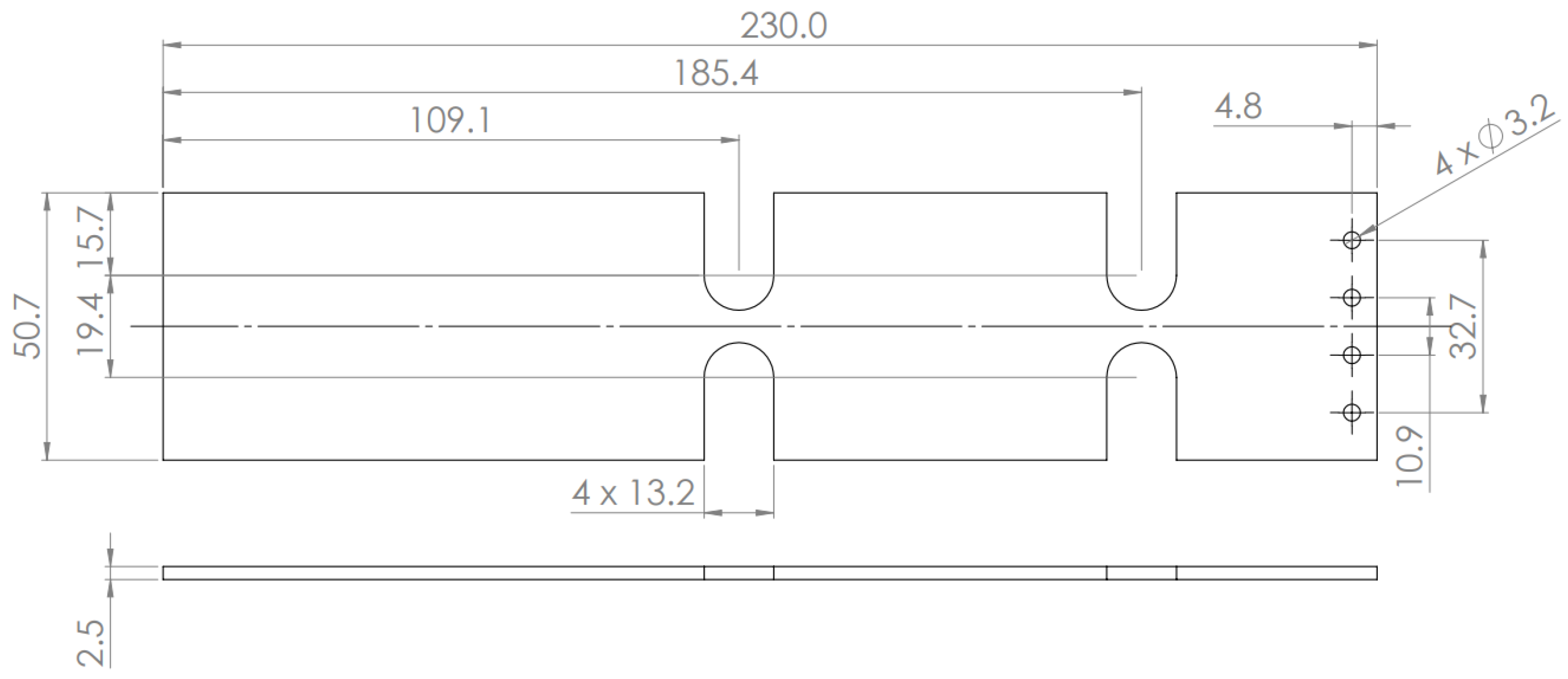
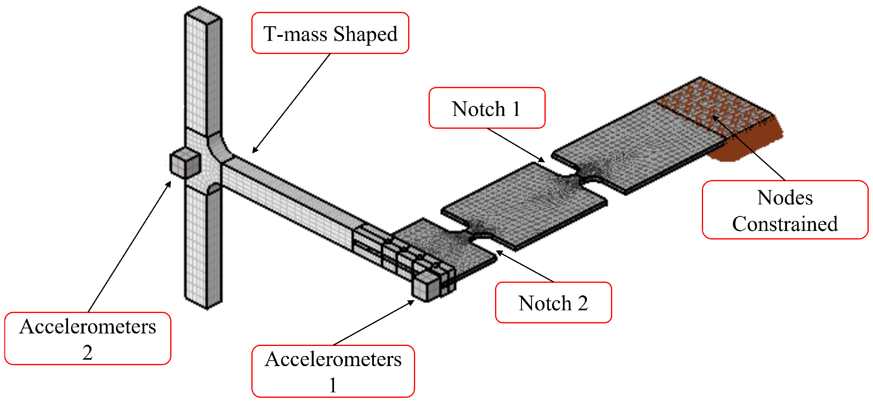
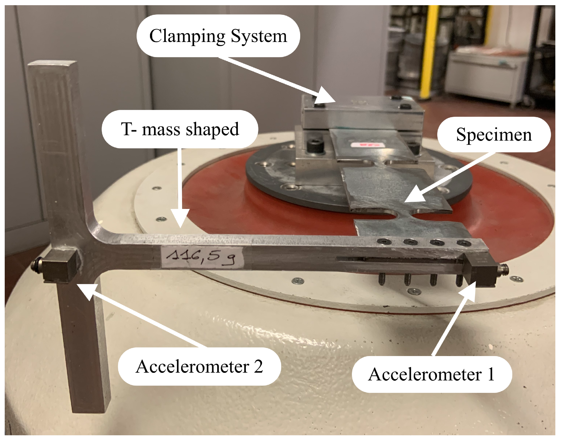
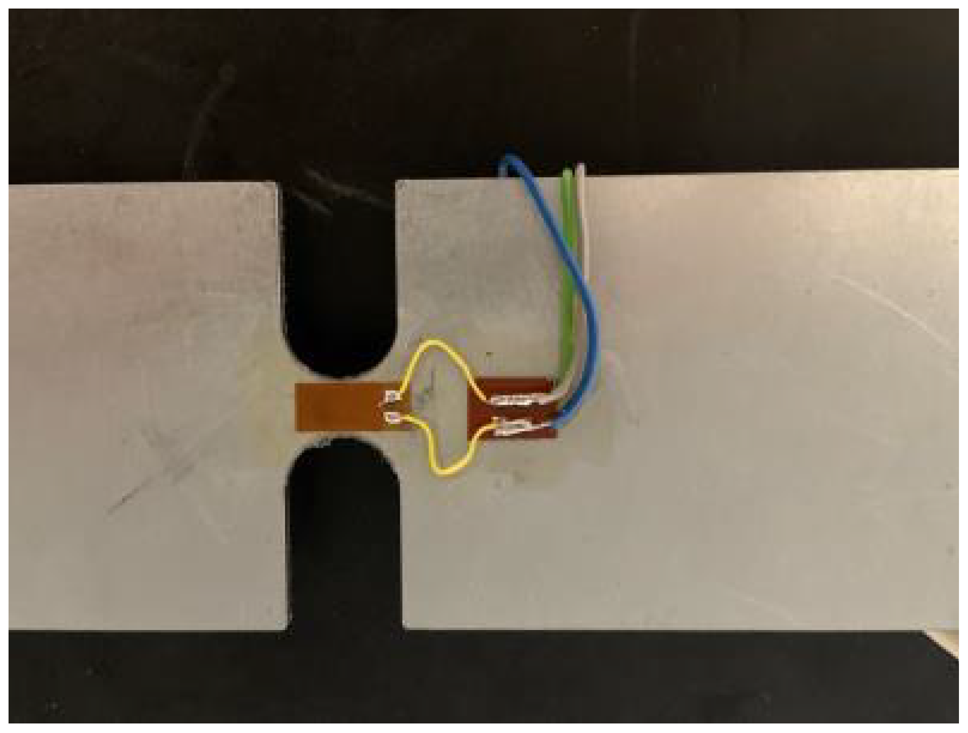
3. Testing Layout
4. Numerical Simulation
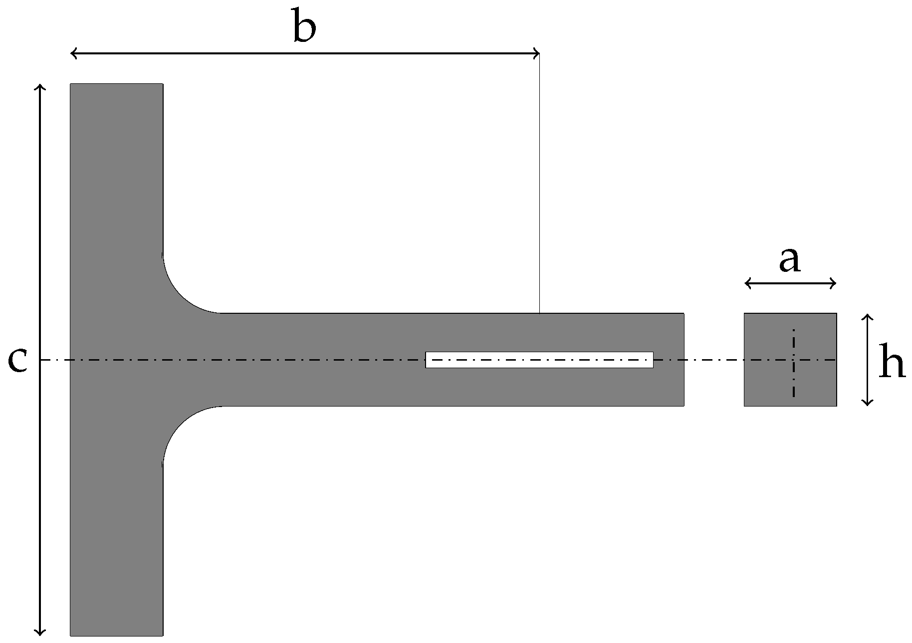
4.1. T-Mass Shaped Design Phase
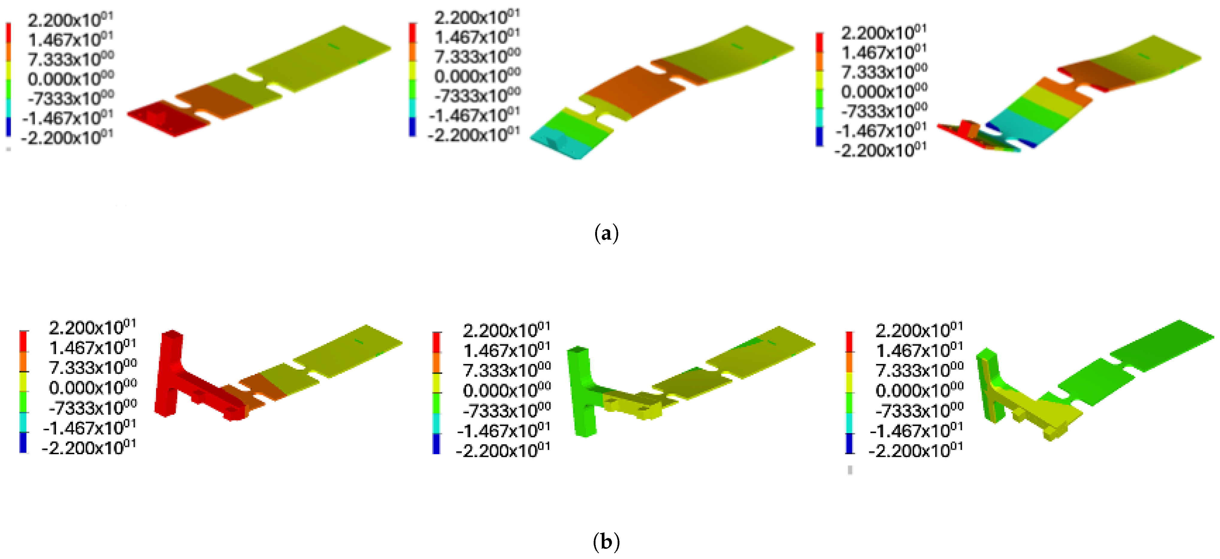
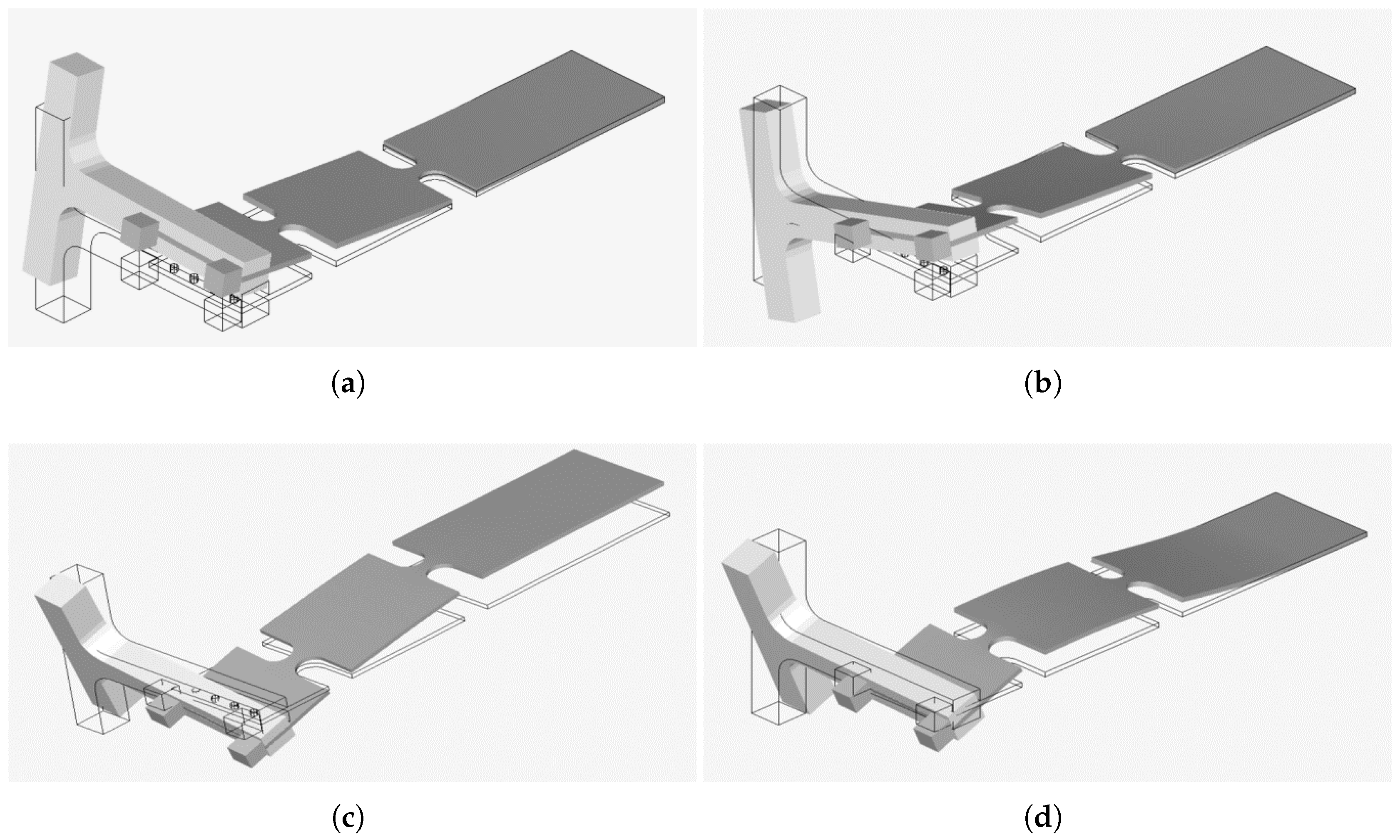
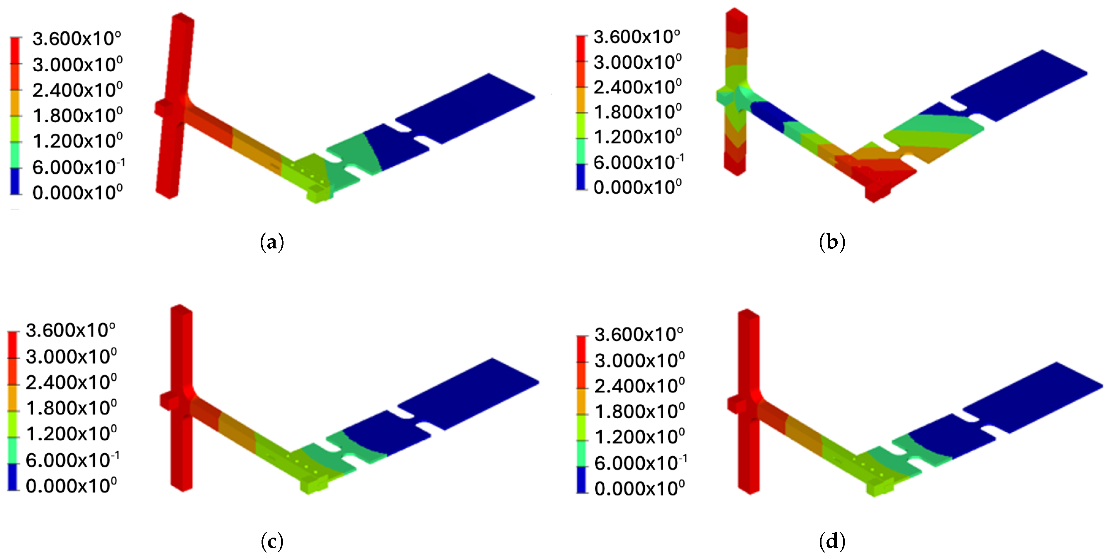
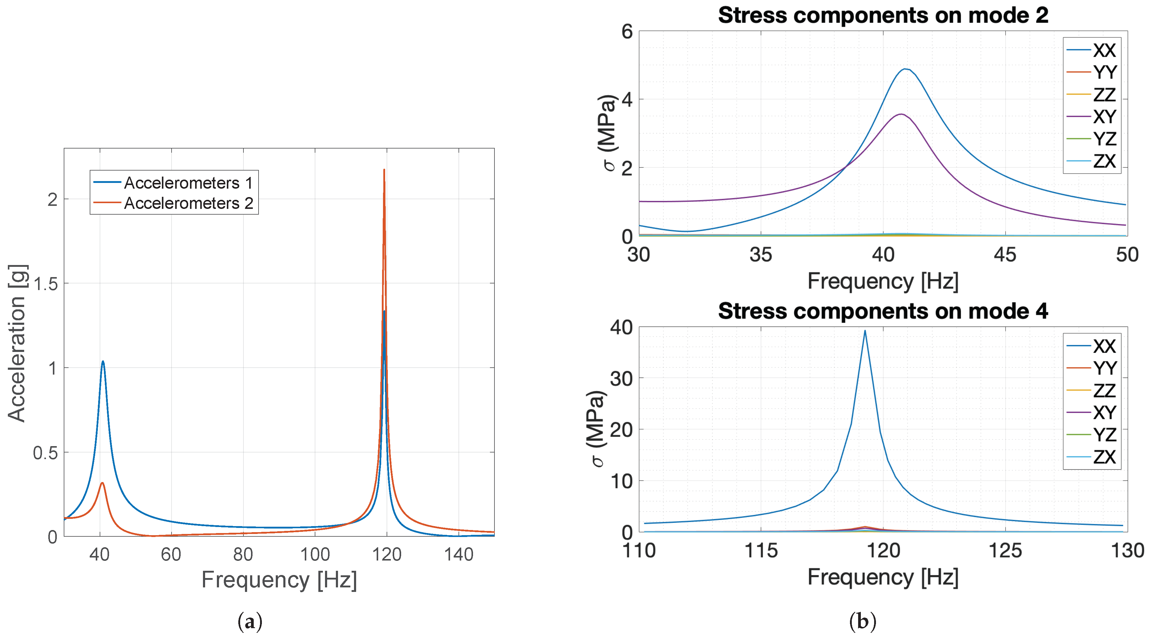
4.2. Dynamic Evaluation
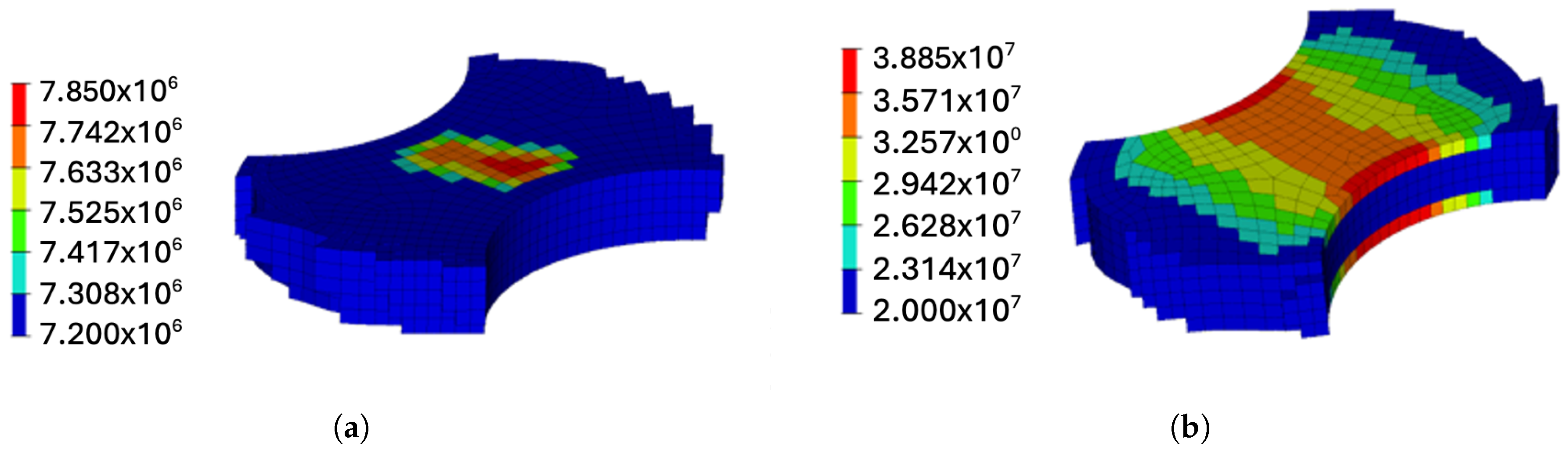
4.3. Fatigue Analysis
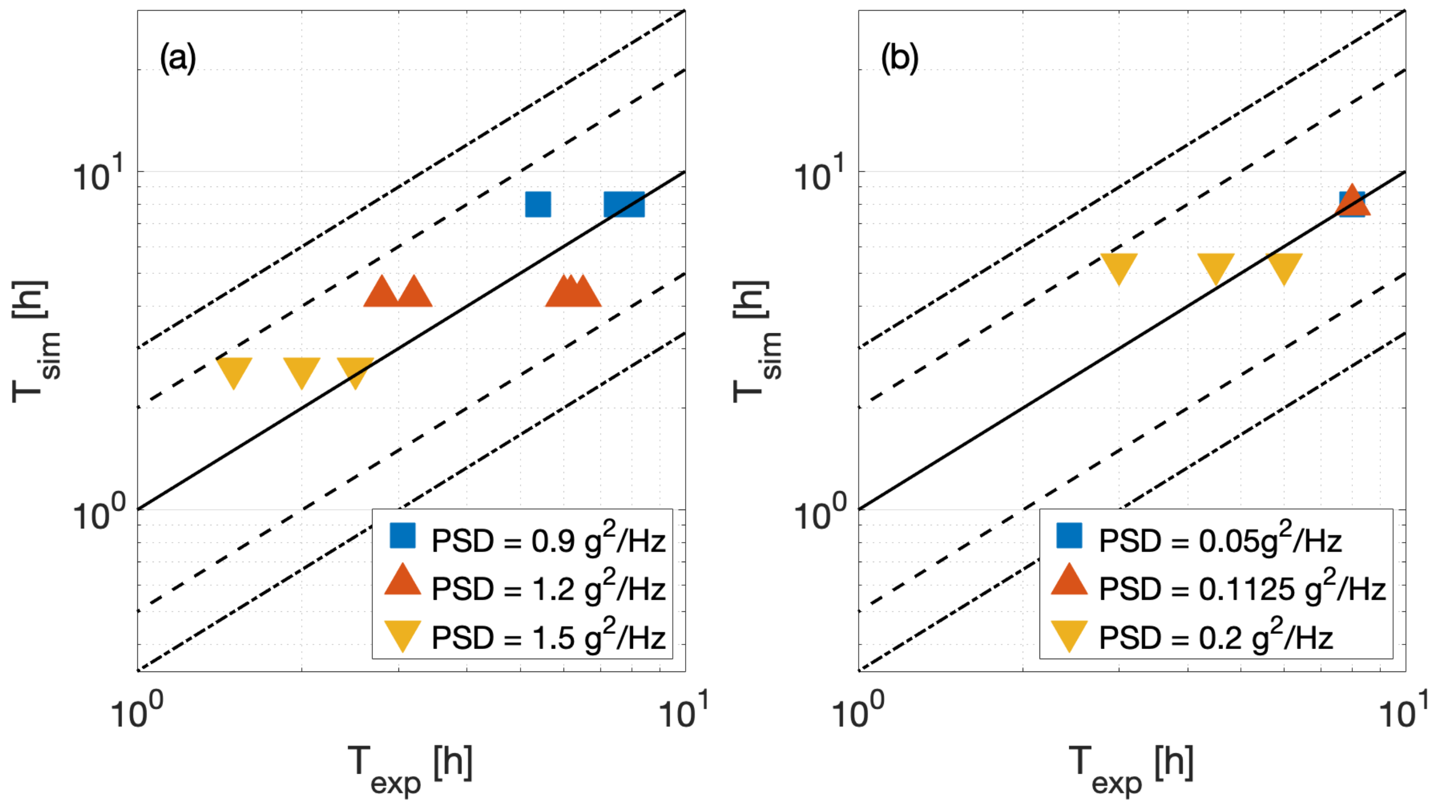
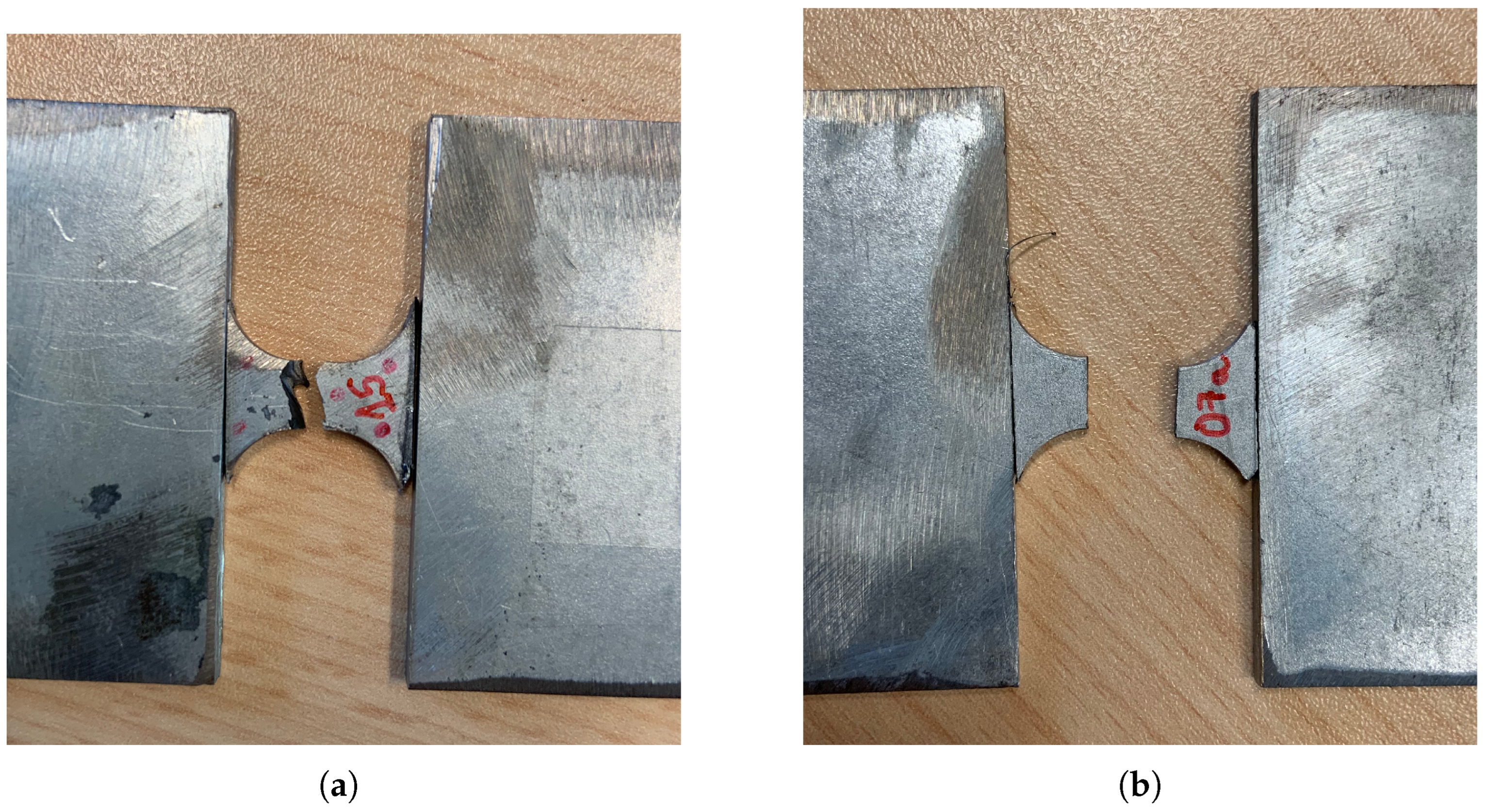
5. Experimental Validation
Random Loading Tests
6. Conclusions
Author Contributions
Funding
Data Availability Statement
Conflicts of Interest
References
- Schijve, J. Fatigue of Structures and Materials; Springer: Berlin/Heidelberg, Germany, 2009. [Google Scholar]
- Sonsino, C.M. Multiaxial fatigue life response depending on proportionality grade between normal and shear strains/stresses and material ductility. Int. J. Fatigue 2020, 135, 105468. [Google Scholar] [CrossRef]
- ASTM E466-21; Standard Practice for Conducting Force Controlled Constant Amplitude Axial Fatigue Tests of Metallic Materials. ASTM International: West Conshohocken, PA, USA, 2021.
- ISO 1099:2017; Metallic Materials—Fatigue Testing—Axial Force-Controlled Method. International Organization for Standardization: Berlin, Germany, 2017.
- DIN 50100:2016-12; Load Controlled Fatigue Testing—Execution and Evaluation of Cyclic Tests at Constant Load Amplitudes on Metallic Specimens and Components. Deutsches Institut für Normung: Geneva, Switzerland, 2016.
- Fatemi, A.; Yang, L. Cumulative fatigue damage and life prediction theories: A survey of the state of the art for homogeneous materials. Int. J. Fatigue 1998, 20, 9–34. [Google Scholar] [CrossRef]
- Liu, Z.; Wang, M.; Guo, P.; Gao, D.; Gao, Y. Numerical and Experimental-Based Framework for Fuel Cell System Fatigue Analysis in Frequency Domain. Machines 2025, 13, 18. [Google Scholar] [CrossRef]
- Shen, K.; Ma, F.; Yuan, J.; Zhang, M. A Damage Combination Method for Fatigue Analysis of Pressure Equipment in Floating Nuclear Power Plants. J. Mar. Sci. Eng. 2025, 13, 236. [Google Scholar] [CrossRef]
- Mršnik, M.; Slavič, J.; Boltežar, M. Multiaxial vibration fatigue—A theoretical and experimental comparison. Mech. Syst. Signal Process. 2016, 76–77, 409–423. [Google Scholar] [CrossRef]
- Carpinteri, A.; Spagnoli, A.; Vantadori, S. A review of multiaxial fatigue criteria for random variable amplitude loads. Fatigue Fract. Eng. Mater. Struct. 2017, 40, 1007–1036. [Google Scholar] [CrossRef]
- Braccesi, C.; Morettini, G.; Cianetti, F.; Palmieri, M. Development of a new simple energy method for life prediction in multiaxial fatigue. Int. J. Fatigue 2018, 112, 1–8. [Google Scholar] [CrossRef]
- Pitoiset, X.; Preumont, A. Spectral methods for multiaxial random fatigue analysis of metallic structures. Int. J. Fatigue 2000, 22, 541–550. [Google Scholar] [CrossRef]
- Habtour, E.; Connon, W.; Pohland, M.; Stanton, S.; Paulus, M.; Dasgupta, A. Review of Response and Damage of Linear and Nonlinear Systems Under Multiaxial Vibration. Shock Vib. 2014, 2014, 294271. [Google Scholar] [CrossRef]
- Appert, A.; Gautrelet, C.; Khalij, L.; Troian, R. Development of a test bench for vibratory fatigue experiments of a cantilever beam with an electrodynamic shaker. In Proceedings of the 12th International Fatigue Congress, Poitiers, France, 27 May–1 June 2018. [Google Scholar]
- Ghielmetti, C.; Ghelichi, R.; Guagliano, M.; Ripamonti, F.; Vezzù, S. Development of a fatigue test machine for high frequency applications. Procedia Eng. 2011, 10, 2892–2897. [Google Scholar] [CrossRef]
- Paulus, M.; Dasgupta, A.; Habtour, E. Life estimation model of a cantilevered beam subjected to complex random vibration. Fatigue Fract. Eng. Mater. Struct. 2012, 35, 1058–1070. [Google Scholar] [CrossRef]
- de M. Teixeira, G. Random vibration fatigue analysis of a notched aluminum beam. Int. J. Mech. Eng. Autom. 2015, 2, 425–441. [Google Scholar]
- Whiteman, W.; Berman, M. Fatigue Failure Results for Multi-Axial Versus Uniaxial Stress Screen Vibration Testing. Shock Vib. 2002, 9, 319–328. [Google Scholar] [CrossRef]
- Whiteman, W.; Berman, M. Inadequacies in Uniaxial Stress Screen Vibration Testing. J. IEST 2005, 44, 20–23. [Google Scholar] [CrossRef]
- French, M.; Handy, R.; Cooper, H. A Comparison of simultaneous and sequential single axis durability testing. Exp. Tech. 2006, 30, 32–37. [Google Scholar] [CrossRef]
- Nath, N.; Aglietti, G.S. Study the effect of tri-axis vibration testing over single-axis vibration testing on a satellite. In Proceedings of the 2022 IEEE Aerospace Conference (AERO), Big Sky, MT, USA, 5–12 March 2022; pp. 1–10. [Google Scholar] [CrossRef]
- Zheng, R.; Liu, C.; Feng, G.; Wei, X.; Chen, H. Spectral decoupled correction algorithm for multi-input multi-output random vibration control. J. Vib. Control 2024, 30, 3797–3805. [Google Scholar] [CrossRef]
- Marques, E.J.; Benasciutti, D.; Niesłony, A.; Slavič, J. An Overview of Fatigue Testing Systems for Metals under Uniaxial and Multiaxial Random Loadings. Metals 2021, 11, 447. [Google Scholar] [CrossRef]
- Morettini, G.; Braccesi, C.; Cianetti, F.; Razavi, N. Design and implementation of new experimental multiaxial random fatigue tests on astm-a105 circular specimens. Int. J. Fatigue 2021, 142, 105983. [Google Scholar] [CrossRef]
- Morettini, G.; Braccesi, C.; Cianetti, F. Experimental multiaxial fatigue tests realized with newly developed geometry specimens. Fatigue Fract. Eng. Mater. Struct. 2019, 42, 827–837. [Google Scholar] [CrossRef]
- Claudio, R.; Reis, L.; Freitas, M. Biaxial high cycl fatigue life assessment of ductile aluminium cruciform specimens. Theor. Appl. Fract. Mech. 2014, 73, 82–90. [Google Scholar] [CrossRef]
- George, T.; Seidt, J.; Shen, M.H.; Nicholas, T.; Cross, C.J. Development of a novel vibration-based fatigue testing methodology. Int. J. Fatigue 2004, 26, 477–486. [Google Scholar] [CrossRef]
- Daborn, P.M.; Ind, P.; Ewins, D. Enhanced ground-based vibration testing for aerodynamic environments. Mech. Syst. Signal Process. 2014, 49, 165–180. [Google Scholar] [CrossRef]
- agoda, T.; Macha, E.; Nieslony, A. Fatigue life calculation by means of the cycle counting and spectral methods under multiaxial random loading. Fatigue Fract. Eng. Mater. Struct. 2005, 28, 409–420. [Google Scholar]
- Nguyen, N.; Bacher-Höchst, M.; Sonsino, C.M. A frequency domain approach for estimating multiaxial random fatigue life. Mater. Werkst. 2011, 42, 904–908. [Google Scholar] [CrossRef]
- Zanellati, D.; Benasciutti, D.; Tovo, R. An innovative system for uncoupled bending/torsion tests by tri-axis shaker: Numerical simulations and experimental results. MATEC Web Conf. 2018, 165, 16006. [Google Scholar] [CrossRef]
- Česnik, M.; Slavič, J.; Boltežar, M. Uninterrupted and accelerated vibrational fatigue testing with simultaneous monitoring of the natural frequency and damping. J. Sound Vib. 2012, 331, 5370–5382. [Google Scholar] [CrossRef]
- Rognon, H. Comportement en Fatique sous Environnement Vibratoire: Prise en Compe de la Plasticite au sein des Methodes Spectrales. Ph.D. Thesis, Ecole Centrale Paris, Châtenay-Malabry, France, 2013. [Google Scholar]
- Bendat, J.; Piersol, A. Random Data: Analysis and Measurement Procedures; Wiley: Hoboken, NJ, USA, 2011. [Google Scholar] [CrossRef]
- Maia, N.; Silva, J. Theoretical and Experimental Modal Analysis; Research Studies Press: Newton, MA, USA, 1997. [Google Scholar]
- Niesłony, A.; Macha, E. Spectral Method in Multiaxial Random Fatigue; Zeszyty Naukowe. Mechanika/Politechnika Opolska; Springer: Berlin/Heidelberg, Germany, 2005; pp. 113–134. [Google Scholar]
- Socie, D.; Marquis, G. Multiaxial Fatigue; SAE International: Warrendale, PA, USA, 1999. [Google Scholar]
- Česnik, M.; Slavič, J.; Čermelj, P.; Boltežar, M. Frequency-based structural modification for the case of base excitation. J. Sound Vib. 2013, 332, 5029–5039. [Google Scholar] [CrossRef]
- Kranjc, T.; Slavič, J.; Boltežar, M. A comparison of strain and classic experimental modal analysis. J. Vib. Control 2014, 22, 371–381. [Google Scholar] [CrossRef]
- Mršnik, M.; Slavič, J.; Boltežar, M. Vibration fatigue using modal decomposition. Mech. Syst. Signal Process. 2018, 98, 548–556. [Google Scholar] [CrossRef]
- Jang, J.; Park, J.W. Simplified vibration PSD synthesis method for MIL-STD-810. Appl. Sci. 2020, 10, 458. [Google Scholar] [CrossRef]
- Pitoiset, X.; Rychlik, I.; Preumont, A. Spectral methods to estimate local multiaxial fatigue failure for structures undergoing random vibrations. Fatigue Fract. Eng. Mater. Struct. 2001, 24, 715–727. [Google Scholar] [CrossRef]
- Miner, M.A. Cumulative Damage in Fatigue. J. Appl. Mech. 2021, 12, A159–A164. [Google Scholar] [CrossRef]
- Mršnik, M.; Slavič, J.; Boltežar, M. Frequency-domain methods for a vibration-fatigue-life estimation—Application to real data. Int. J. Fatigue 2012, 47, 8–17. [Google Scholar] [CrossRef]
- Milella, P.P. Fatigue and Corrosion in Metals; Springer Science & Business Media: Berlin/Heidelberg, Germany, 2012. [Google Scholar]
- Nagulapalli, V.; Gupta, A.; Fan, S. Estimation of fatigue life of aluminum beams subjected to random vibration. In Conference Proceedings of the Society for Experimental Mechanics Series; Springer: Berlin/Heidelberg, Germany, 2007. [Google Scholar]


| Component | Material | E [GPa] | Density [kg/m3] |
|---|---|---|---|
| Specimen | Steel | 200 | 7740 |
| T-mass | Aluminum | 72 | 2715 |
| T-Mass Configuration | a [mm] | b [mm] | c [mm] | h [mm] | Mass [g] |
|---|---|---|---|---|---|
| 1 | 14.9 | 86.7 | 90.0 | 15.0 | 106.9 |
| 2 | 11.0 | 130.00 | 135.0 | 12.7 | 106.9 |
| 3 | 9.5 | 151.73 | 157.5 | 12.0 | 106.9 |
| Mode 1 | Mode 2 | Mode 3 | Mode 4 | |||||
|---|---|---|---|---|---|---|---|---|
| [Hz] | Shift | [Hz] | Shift | [Hz] | Shift | [Hz] | Shift | |
| 1 | 20.29 | 62.28 | 88.18 | 169.82 | ||||
| 2 | 17.98 | 44.80 | 72.59 | 135.59 | ||||
| 3 | 16.82 | 40.85 | 63.31 | 119.20 | ||||
| Mode 1 | Mode 2 | Mode 4 | ||||
|---|---|---|---|---|---|---|
| Shift | Shift | Shift | ||||
| 1 | 0.436 | 0.0869 | 0.189 | |||
| 2 | 0.416 | 0.139 | 60.1 | 0.190 | 0.3 | |
| 3 | 0.340 | 0.166 | 86.0 | 0.193 | 1.7 | |
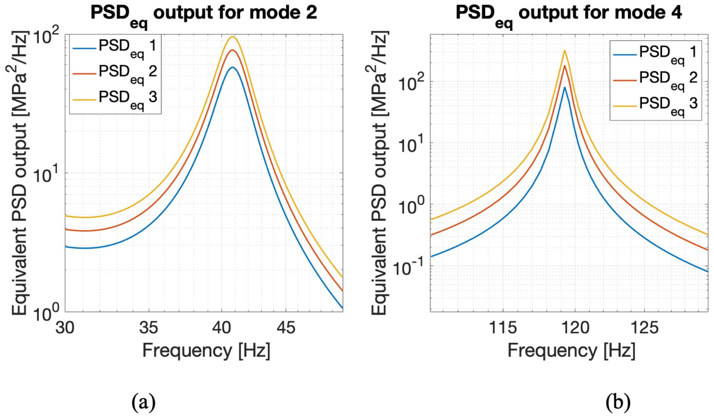
| Mode 2 | Mode 4 | |||
|---|---|---|---|---|
| [MPa] | Shift | [MPa] | Shift | |
| 1 | 2.98 | 27.35 | ||
| 2 | 6.24 | 109 | 35 | 27 |
| 3 | 7.85 | 163 | 38.85 | 42 |
| Mode | Frequency [Hz] | Deformation |
|---|---|---|
| 1 | 16.9 | bending |
| 2 | 40.85 | torsional–bending |
| 3 | 63.31 | bending |
| 4 | 119.82 | bending |
| Mode | [%] |
|---|---|
| 2 | 3 |
| 4 | 1.5 |
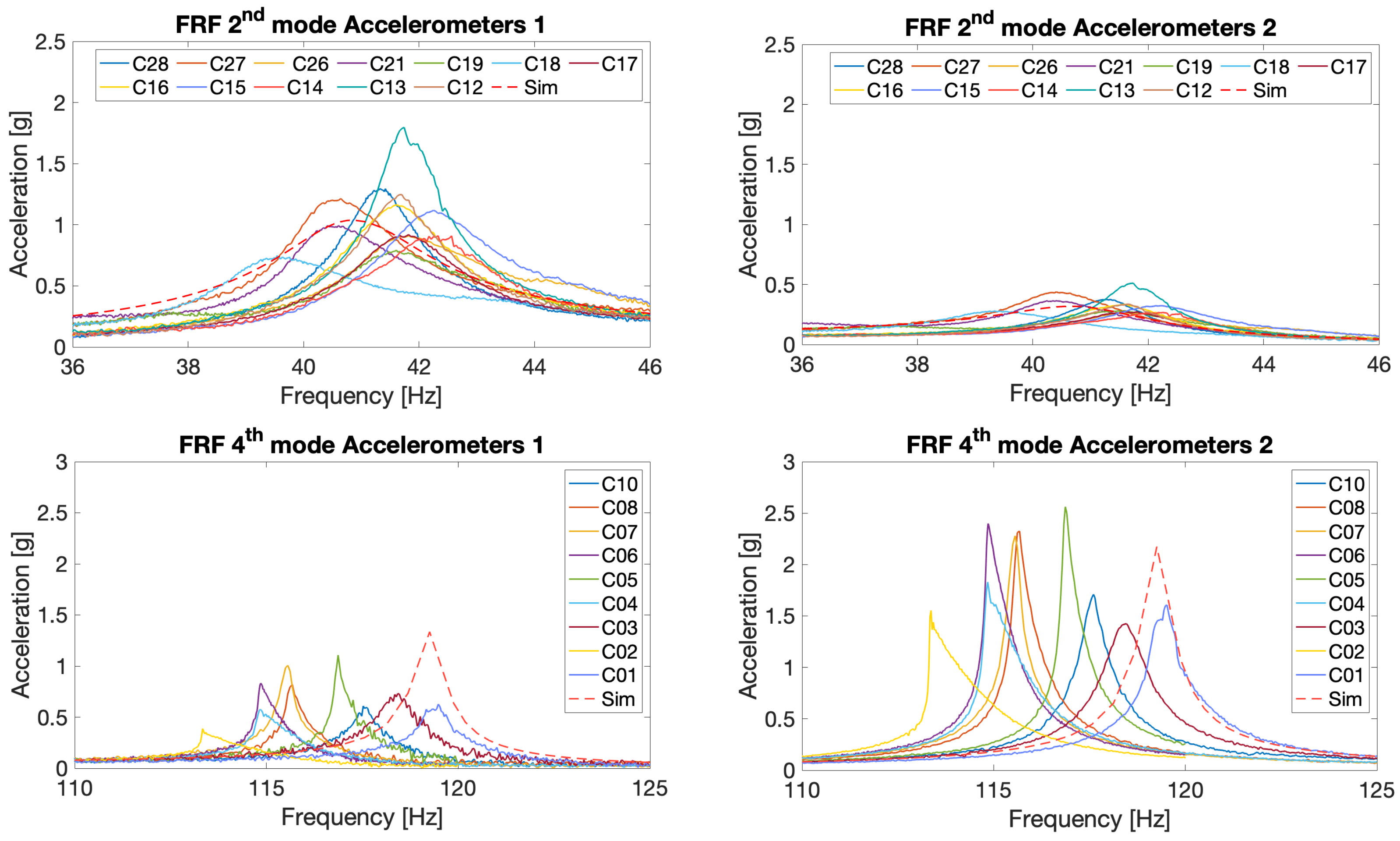
| Mode 2 | Mode 4 | |
|---|---|---|
| Accelerometer 1 [g] | 1 | 1.3 |
| Accelerometer 2 [g] | 0.34 | 2.2 |
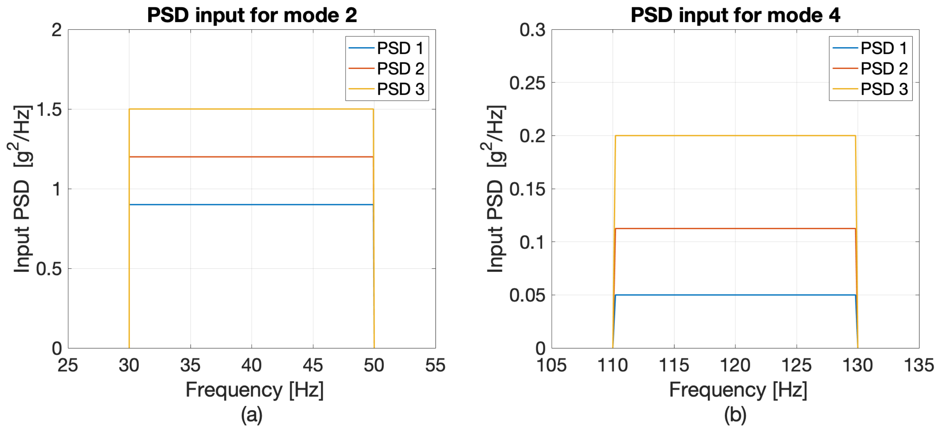
| Mode 2 | Mode 4 | |||||
|---|---|---|---|---|---|---|
| PSD [g2·Hz−1] | 0.9 | 1.2 | 1.5 | 0.05 | 0.112 | 0.2 |
| RMS [g] | 4.2 | 4.9 | 5.5 | 1 | 1.5 | 2 |
| Mode | Accelerometer 1 [g] | Accelerometer 2 [g] |
|---|---|---|
| 1 | 1.1 | 0.3 |
| 2 | 0.7 | 2 |
Disclaimer/Publisher’s Note: The statements, opinions and data contained in all publications are solely those of the individual author(s) and contributor(s) and not of MDPI and/or the editor(s). MDPI and/or the editor(s) disclaim responsibility for any injury to people or property resulting from any ideas, methods, instructions or products referred to in the content. |
© 2025 by the authors. Licensee MDPI, Basel, Switzerland. This article is an open access article distributed under the terms and conditions of the Creative Commons Attribution (CC BY) license (https://creativecommons.org/licenses/by/4.0/).
Share and Cite
Campello, L.; Denis, V.; Sesana, R.; Delprete, C.; Serra, R. New Experimental Single-Axis Excitation Set-Up for Multi-Axial Random Fatigue Assessments. Machines 2025, 13, 539. https://doi.org/10.3390/machines13070539
Campello L, Denis V, Sesana R, Delprete C, Serra R. New Experimental Single-Axis Excitation Set-Up for Multi-Axial Random Fatigue Assessments. Machines. 2025; 13(7):539. https://doi.org/10.3390/machines13070539
Chicago/Turabian StyleCampello, Luca, Vivien Denis, Raffaella Sesana, Cristiana Delprete, and Roger Serra. 2025. "New Experimental Single-Axis Excitation Set-Up for Multi-Axial Random Fatigue Assessments" Machines 13, no. 7: 539. https://doi.org/10.3390/machines13070539
APA StyleCampello, L., Denis, V., Sesana, R., Delprete, C., & Serra, R. (2025). New Experimental Single-Axis Excitation Set-Up for Multi-Axial Random Fatigue Assessments. Machines, 13(7), 539. https://doi.org/10.3390/machines13070539