Condition-Based Maintenance for Degradation-Aware Control Systems in Continuous Manufacturing

Abstract

To enhance maintenance endeavors, it is imperative to gain a deep understanding of system degradation. In systems with degradation-aware control, observing degradation becomes particularly challenging. Even with sensors, such controllers continuously mitigate deviations to ensure the system operates within optimal limits. Here, we propose a framework explicitly tailored for degradation-aware control systems, built upon two main components: (1) degradation modeling to estimate and track hidden degradation over time and (2) a Long Short-Term Memory Autoencoder-Degradation Stage Detector (A-LSTMA-DSD) to define alarm and failure thresholds for enabling condition-based maintenance. In degradation modeling, the framework utilizes actuator measurements to model hidden degradation. Next, an A-LSTMA-DSD model is developed to flag anomalies, based on which alarm and failure thresholds are assigned. These dynamic thresholds are defined to ensure sufficient time for addressing maintenance requirements. Working with real data from a boiler unit in an oil refinery and focusing on steam leakages, our proposed framework successfully identified all failures and on average triggered alarm and failure thresholds 15 and 8 days in advance of failures, respectively. In addition to triggering these thresholds, our system outperforms baseline models, such as CNN, LSTM, ANN, ARIMA, and Facebook Profit, in identifying failures by 60% and 95%, respectively.

1. Introduction

Condition-based maintenance (CBM) revolutionizes maintenance practices by leveraging the real-time monitoring and analysis of equipment conditions. Unlike traditional fixed schedules, CBM utilizes cutting-edge sensors and monitoring technologies to gather data on machinery health, identify early signs of deterioration, and predict potential failures. This proactive approach enables organizations to schedule maintenance precisely when needed, leading to cost savings, enhanced reliability and uptime, improved safety, increased productivity, and optimized asset performance. In essence, CBM represents a strategic shift towards smarter and more efficient maintenance management practices, offering unparalleled benefits across diverse industries.

Maintenance entails the restoration of a subsystem or system to a satisfactory condition to enhance reliability and efficiency after prolonged use [1]. This process involves a blend of managerial, technical, and administrative activities [1]. The importance of maintenance has been emphasized for its role in enhancing cost effectiveness, availability, process quality, and safety compliance [2,3]. Maintenance costs constitute a significant part of the operating budget of plants, taking up to 70% of total costs [4,5]. In many industries, the ratio of maintenance costs to added value is more than 25% [6]. Maintenance strategies, as shown in Figure 1, can be broken into corrective or preventive. While corrective maintenance (e.g., palliative and curative) is conducted after the damage is detected to restore an asset to a functional state, preventive maintenance is proactive and based on expected lifespan and historical performance data, aiming to prevent failures by addressing potential issues before their occurrence. Preventive maintenance is further divided into systemic, condition-based, and predictive maintenance. Systemic maintenance involves performing maintenance tasks at predetermined intervals or based on established criteria to prevent failures. CBM relies on the real-time monitoring and analysis of equipment conditions to schedule maintenance activities precisely when needed [7].

Given that at its core maintenance is about restoring a degraded entity to a useful state [8], degradation modeling is a major step in CBM [9]. Degradation within a system can be modeled by describing its effects on the system’s performance and examining the reverse impacts of operations on degradation [10]. Physical variables (e.g., temperature and humidity) and operational modes (e.g., sequencing of recipes in a batch process), are examples of elements that can affect degradation [11]. Physics-based, statistical, heuristic, data-driven, and hybrid modeling are distinct types of degradation models.

The categorization of degradation models is based on the input parameters and their dependency behavior, regardless of their specific type (e.g., physical or data-driven) [12]. A degradation-dependent model is necessary when degradation affects either the system’s inputs or outputs, while a degradation-independent model is applicable when degradation has no impact on the system. This modeling may be factor-free or factor-based. While factor-based models depend on influencing factors (e.g., operating mode), factor-free models are independent of any factors, as suggested by their names [13].

The degradation-aware control strategy adjusts system performance in real time as components degrade. By compensating for this degradation, the system continues operating within its desired parameters, ensuring smooth and efficient functioning. However, this constant adjustment can make early-stage failure detection (or even close to the final stages) more difficult, as the system actively masks the effects of deterioration to maintain performance. In recent years, degradation-based reliability analysis has gained popularity, as evidenced by the growing importance of rapid degradation testing [14]. Remaining Useful Life (RUL) and degradation modeling have been the focus of several studies. Ref. [15] concentrated on statistical data-driven strategies for estimating RUL, while [16] explained degradation models as stochastic processes. Ref. [17] reviewed degradation-model-based RUL estimation methodologies for heterogeneous systems. Ref. [14] reviewed degradation-aware control systems from a design optimization perspective. These works have all highlighted the need for further research on system degradation in degradation-aware systems.

Real-time reliability evaluation and prediction have become increasingly essential over the past two decades, particularly in CBM [18,19,20,21]. Regression analysis and time series forecasting are the primary methodologies used in real-time reliability evaluation and prediction [22]. While some studies explored the use of Bayesian methods [23,24,25], others utilized neural networks [26,27,28].

Additionally, fault-tolerant control has been widely studied in the literature [29,30,31,32,33,34,35,36]. For instance, [37,38] created model-based optimizing control for a compressor station. Ref. [39] incorporated behavior and gray-box models to predict and control the temperature of Melton steel with high accuracy in a steel-making process. Although their proposed model improved the performance of a feed-forward controller, the authors were unable to ameliorate the degradation [39].

Given the high implementation rate of Machine Learning (ML) and Artificial Intelligence (AI) in different areas such manufacturing [40,41], healthcare [42,43,44], environment [44,45], and agriculture [46,47], growth in using deep learning techniques is expected, such as Long Short-Term Memory (LSTM) networks, bidirectional LSTM networks, and Deep Convolution Neural Networks for RUL and fault detection for infrastructure and machinery systems [48,49,50,51,52,53].

Most existing CBM studies assume that degradation is a monotonic function and that the system needs to be maintained once it reaches a predefined threshold [2,34,35,36,37]. Degradation-aware control systems have subsystems competing to survive failure by alleviating the degradation under controller compensation influence. For example, leak degradation may occur during the heat exchange process in a heat exchanger. The level of performance will be compensated by a Pressure Indicator Controller (PIC) to keep the system pressure within the required range, as illustrated in Figure 2. Because of this compensation, the system will continue to operate at a consistent level, and the measurement remains within a predetermined range. Failure will happen either because the controller can no longer compensate for the degraded characteristic or because other operation and management thresholds are violated, like safety requirements.

Here, we propose a conditionally maintained, degradation-aware control system. Such a system accounts for component wear and aging, enabling more informed and efficient decision making, where the control mechanism operates by continuously monitoring the system’s output and adjusting control inputs in real time to optimize performance, while improving the RUL by scheduling maintenance as needed. The framework functions by tracking the hidden degradation through degradation-dependent modeling and detecting degradation stages to determine dynamic alarm and failure thresholds. The alarm threshold is an early warning level set to indicate that an asset is experiencing abnormal conditions and may require maintenance soon. When a monitored parameter, such as pressure, exceeds this threshold, it signals potential degradation, allowing maintenance teams to take proactive action. If no intervention occurs and the condition continues to worsen, the asset may reach the failure threshold, which is the point at which it can no longer perform optimally and is at risk of a complete breakdown. The gap between these thresholds is crucial for effective maintenance planning, as it provides time to address issues before they lead to unexpected failures, ensuring reliability and cost efficiency in operations.

The rest of the paper is organized as follows. Section 2 outlines the proposed framework, focusing on degradation modeling and threshold setup. Section 3 describes the system components and their role in reliability. Section 4 presents results showing how the model tracks degradation and sets thresholds to prevent breakdowns. Section 5 concludes that the framework effectively tracks degradation and sets dynamic thresholds in advance.

2. Materials and Methods

Our proposed framework is depicted in Figure 3. This framework has two main components: (1) degradation modeling and (2) threshold setup. While the degradation modeling relies on tracking the hidden degradation buildups over time based on the controller compensation, the second step focuses on classifying different degradation stages for setting up the alarm and, subsequently, failure thresholds.

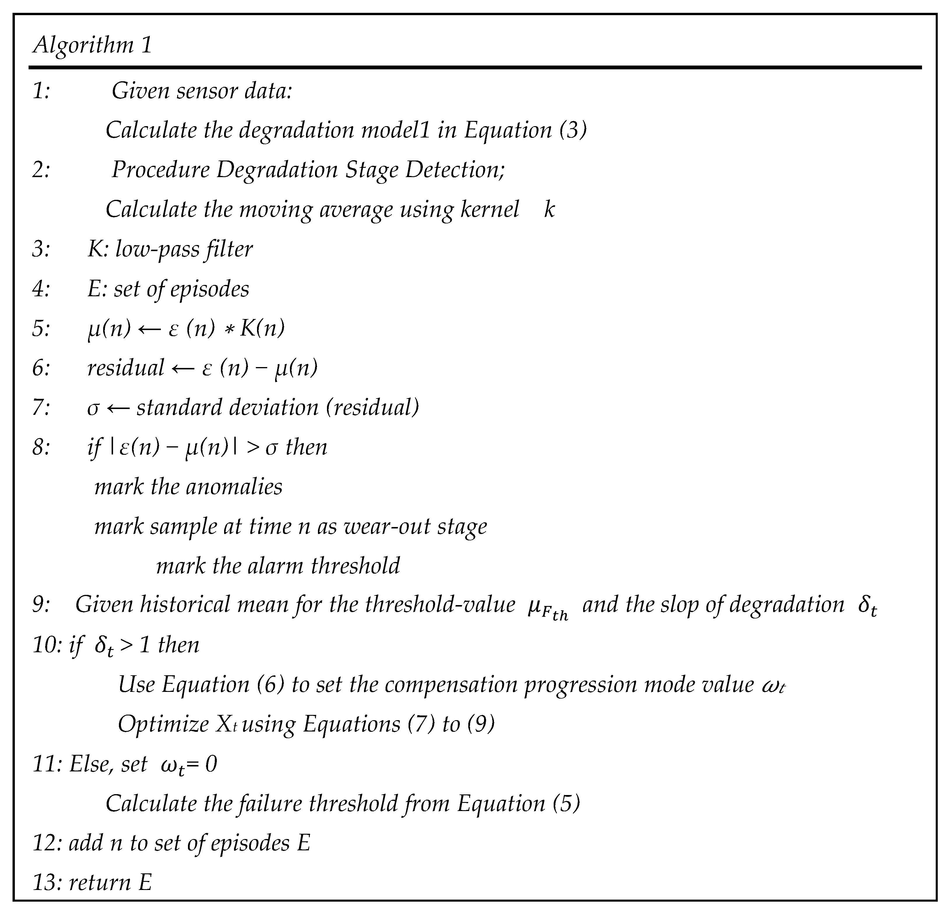
2.1. Degradation Modeling

The goal of this section is to model and track hidden degradation buildups. Our proposed degradation-dependent model assumes that the impacts of degradation on system variables, inputs, and outputs are measurable through the control system’s compensation. The term compensation is defined in this work as the quantity that is needed to be adjusted to offset the value change in the system because of escalated failure [54,55]. We assume that this magnitude of compensation is an indicator of the degradation progression in the degradation-aware systems. Figure 3 displays the steps for modeling the degradation path. These steps include data pre-processing (Figure 4), model fitting, and an adequacy check.

The first step in degradation modeling is data pre-processing, which is displayed in Figure 4. The data are extracted from a data collection unit in the data management system of an oil refinery. During the cleaning process, any unnecessary symbols or letters are removed to ensure proper formatting. Once cleaned, the data are imputed to address missing values and are scaled. Next, the pre-processed data are used to fit our proposed model to discover a degradation path through Equations (1)–(3).

$$D_{i,t}=D_{i,t-1}+\left(M_{i,t}-{SP}_i\right)+{\epsilon }_{i,t} \forall i\in \left\{\mathrm{1,2},\dots ,I\right\}\forall t\in \left\{1,2,\dots ,T\right\},$$

(1)

$D_{i, t}$ is the accumulated degradation of controller i at time t (i = 1…I and t = 1…T), ${SP}_i$ is the set point for the ith controller, $M_{i,t}$ is the measurement of the controller i at time t, and ${\epsilon }_{i,t}$ is the stochastic error with an assumed mean of zero and a time-invariant variance of ${\mathsf{\sigma }}_i^2$, independently distributed across different time periods t = 1…T for each controller i = 1…I. Replacing deterioration at times $t-1, t-2,\dots ,1$ with their corresponding definitions, we can obtain Equation (2).

$$D_{i,t}={\sum }_{t=1}^T\left(M_{i,t}-{SP}_i+{\epsilon }_{i,t}\right) \forall i\in \left\{1,2\dots ,I\right\}$$

(2)

which could be further simplified to Equation (3):

$$D_{i,t}=-T\times {SP}_i+{\sum }_{t=1}^T\left(M_{i,t}\right)+E_i \forall i\in \left\{\mathrm{1,2},\dots ,I\right\}$$

(3)

where ${\sum }_{t=1}^T{SP}_i=-T {\times SP}_i$ and $E_i=\sum _{t=1}^T{\epsilon }_{i,t}$ is a stochastic process with a mean of zero and variance ${\displaystyle \frac{{\mathsf{\sigma }}_i^2}{T}}.$ In degradation-aware control systems, the controller offsets any divergence and disturbance from a predefined set point [56,57,58,59], and stochastic noise and disturbance are undeniable. In our proposed model, the error represents the indirect effects of environmental noise, signal transients, and variations due to monitoring equipment. Our main assumption is that the error is normally distributed with a mean of zero and a time-invariant variance. The adequacy step checks the normality of the error along with having a mean of zero and constant variance assumptions.

2.2. Threshold Setup

The next stage of our proposed framework focuses on threshold setup, which aims to define alarm and failure thresholds based on the output of degradation modeling. First, a Long Short-Term Memory Autoencoder (A-LSTM) deep neural network is developed to detect early abnormal behaviors in the degradation path. Our A-LSTM model consists of one input layer (reading the degradation trends), followed by two stacked LSTM layers (as displayed in Figure 5), a repeat vector layer, two additional stacked LSTM layers, and a final dense layer.

While the stacked LSTM layers are embedded to handle the sequential data more accurately, the repeated vector layer feeds the encoder and decoder sections of the network. Because of the structure of LSTMs, the network can learn short- and long-term dependencies while solving the vanishing-gradient problem that affects traditional Recurrent Neural Networks [37]. The encoder in the autoencoder network (Figure 6) translates the sequence data into a vector; then, the decoder reverses the process by translating the vector into a sequence. During this process, the architecture can capture anomalies, which flags the alarm threshold.

After modeling degradation behavior, degradation stage detection is achieved by investigating the data reconstruction and catching any increase in the mean squared error (MSE) via A-LSTM. The algorithm is trained on 13 episodes in which different states of degradation are observed. Our proposed degradation stage detection framework (Figure 3) ties together degradation modeling and degradation stage detection, where the output of degradation modeling is fed to our developed A-LSTM network to define alarm and failure thresholds.

The proposed Alarm Setting Algorithm, as displayed in Figure 7, initiates degradation modeling by utilizing the degradation model proposed in Equation (3). Then, a fixed window is placed on the normalized time series data to measure the degradation compensation in the controller. This window is placed based on a group time sequence of events. The values for the alarm and failure thresholds are determined through Algorithm in Figure 7. First, the model is trained to detect anomalies, and when an anomaly is detected, it triggers the alarm threshold, $A_{th}$, marking the start of the wear-out stage, which indicates the first sign of degradation. Following this, the failure threshold, $F_{th}$, is calculated based on the alarm threshold and the historical mean of previously detected failure thresholds. The failure threshold is defined according to the severity of the degradation pattern, as described in Equations (4)–(6). In essence, the alarm threshold signals the initial detection of degradation, while the failure threshold identifies the point of critical system failure.

$$F_1=A_{th}+{\mathsf{\mu }}_{F_{th}}-{\omega }_t\times Pen$$

(4)

$$F_t=F_{t-1}-{\omega }_t\times Pen$$

(5)

$${\omega }_t=X_t({\delta }_t-1)$$

(6)

where $F_1$is the first failure threshold, defined as the alarm threshold plus the ${\mathsf{\mu }}_{F_{th}}$ (i.e., the mean value for failure thresholds from the historical data) and adjusted based on ${\omega }_t$ and ${\delta }_t$; ${\omega }_t$ is the parameter that shows the compensation progression mode at time t; ${\mathsf{\delta }}_t$ is the slope of the compensation accumulation at time t; and $X_t$ is the binary decision variable indicating whether the failure threshold should be more aggressive, triggering the failure threshold sooner. The value of $X_t$ should be 1 if the degradation slope is larger than the predefined threshold of the previous episodes and 0 otherwise.

$$Max X_t$$

(7)

This is subject to the following:

$$\left({\mathsf{\delta }}_t-1\right)X_t\ge 0$$

(8)

$$X_t\in \{0, 1\}$$

(9)

Equation (7) is pushing $X_t$ to be one. If the slope is downward (i.e., ${\delta }_t$ < 1), Xt would be zero because of Equation (8). This translates to no need to trigger the failure threshold sooner due to slow degradation. As soon as the degradation becomes aggressive (i.e., ${\delta }_t$ ≥ 1), $X_t$ will be pushed to be one by Equations (7)–(9). At this point, continuous monitoring of the system is suggested, and a faster triggering of the failure threshold would take place considering the degradation progression with the calculation of weight (${\omega }_t$) and penalty (Pen) parameters. Figure 7 illustrates the Alarm Setting Algorithm, which oversees the definitions of alarm and failure thresholds.

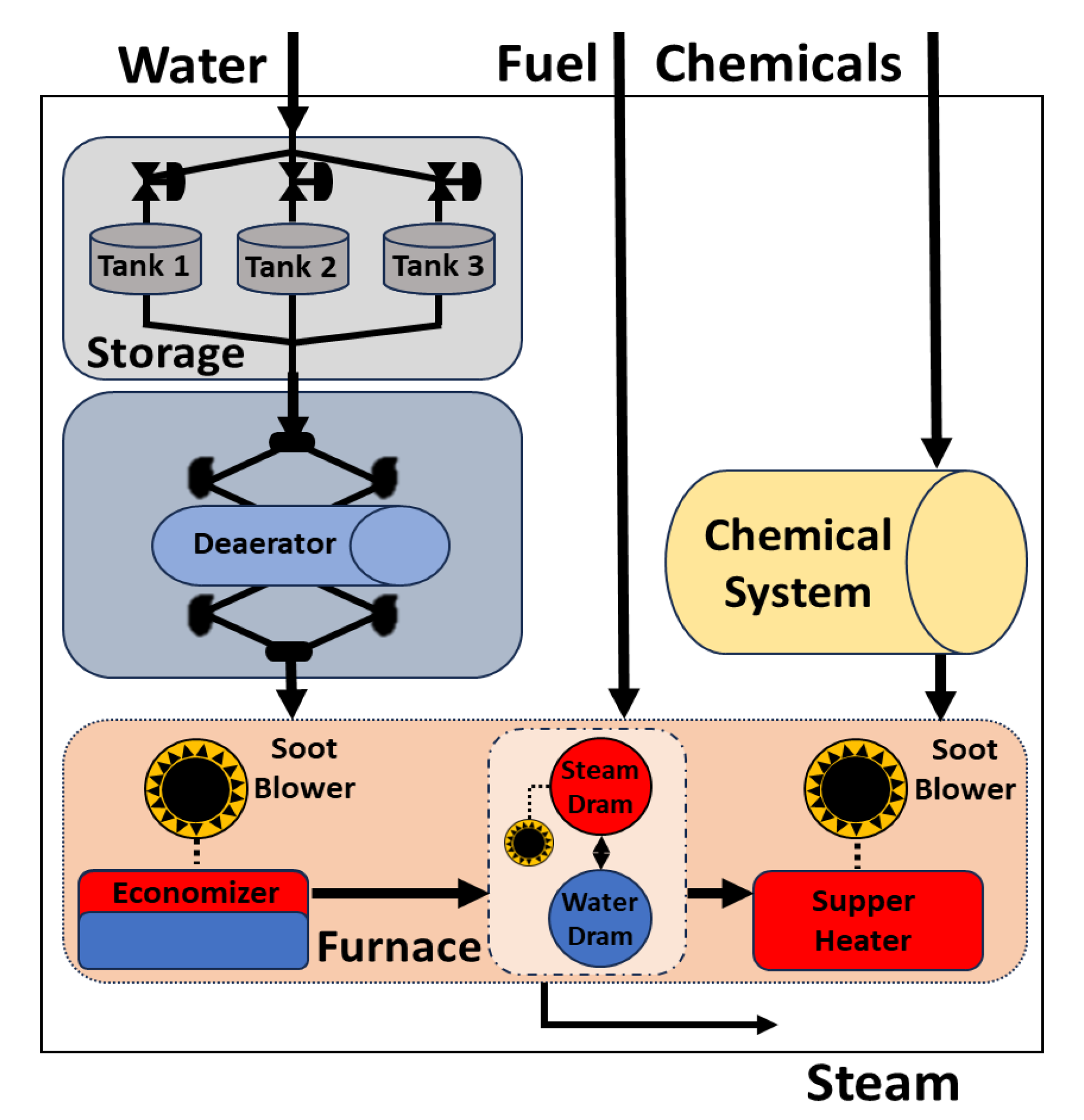
3. System Description

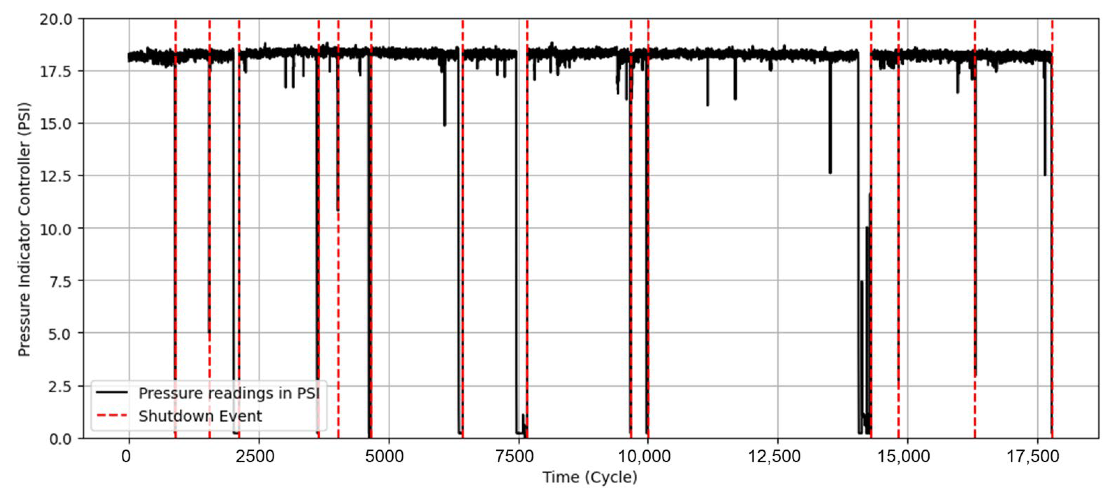
As depicted in Figure 8, the system under study is made of three main units: storage, chemicals, and furnace. The storage unit stores water in three tanks, and the deaerator equipment separates gases from water. This separation prepares water for the last destination, which is the furnace. Some chemicals are processed in parallel to be injected into the furnace to improve its performance. As displayed in Figure 8, while storage and deaerators have redundant parts to improve the reliability of the system, the furnace lacks such design due to high costs. As a result, the furnace is the most crucial part of the boiler system and has the most failure percentage, leading to shutdowns. Breaking any item can cause a general breakdown, as there is no redundant subsystem for the furnace.

Dataset

In this study, data were collected from the Distributed Control System (DCS) of an oil refinery’s boiler unit. The key parameters include the pressure, boiler level, fuel oil flow, super-heated steam flow, and steam temperature along with 11 managerial features. Of these, pressure is the most critical parameter, as it plays a significant role in system performance and failure detection. Pressure readings were measured in PSI (pounds per square inch) at intervals of 98 min and were sourced directly from the DCS. Over the course of three years, we gathered 17,030 data points. This dataset spans 14 episodes, as displayed in Figure 9.

Figure 9 displays the controller output signal alongside the PIC measurements across these 14 episodes. The PIC readings for the first 13 episodes are essentially the inputs used for training the proposed framework. Each episode is marked by the vertical dotted red lines. These red lines indicate the incidents of emergency shutdowns during the study period, providing a clear visual reference for when these events occurred in relation to the overall performance of the boiler system. For example, Episode 11 has the longest time to failure at 287 days. The data are sent to the control room and the PLC unit, which helps keep track of the boiler’s condition and optimize its performance.

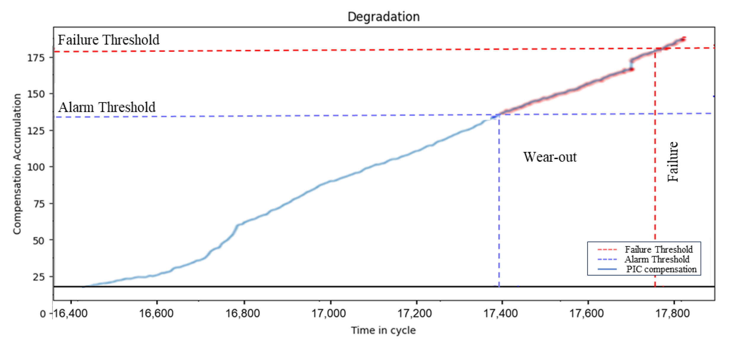
4. Results and Discussion

The first thirteen episodes were utilized for training, while the fourteenth episode served as the test set. Our proposed framework demonstrates the precise identification of gradual degradations (such as leaks) across both the training (first thirteen episodes) and test (episode fourteen) datasets. Given the rarity of failure events in large boiler units at oil refineries, data collection for such scenarios is both challenging and costly. Furthermore, as the data are sourced from a functioning refinery, collection is constrained by operational factors. The 13:1 training-to-testing ratio ensures a sufficient amount of training data while supporting effective generalization. Despite the limited number of episodes, the extended duration of the dataset, coupled with the dynamic nature of the system, enabled the identification of significant degradation patterns, resulting in a robust model that provides reliable predictions. Thus, although fewer episodes were available, the depth and diversity of the data collected over three years formed a solid foundation for model performance.

To validate the proposed framework, the results of the degradation modeling and the overall framework are compared against ground truth data, including PIC readings and recorded failure events over the study period. The degradation detection results exhibit strong agreement with commonly observed failure patterns throughout a system’s lifecycle, namely the childhood, adulthood, and wear-out phases. In the childhood phase, early instability arises due to manufacturing defects or improper installation. Once these initial instabilities are addressed, the system enters the adulthood phase, characterized by a period of stability with infrequent and random failures. Eventually, the system progresses into the wear-out phase, where failure rates increase due to the cumulative effects of wear and tear under operational conditions.

To illustrate the effectiveness of the proposed framework, we present its application in Episode 14. Figure 10 visualizes the degradation stages identified by the hidden degradation model, along with the corresponding alarm and failure thresholds. In Episode 14, the system initially exhibits slight volatility, indicating early instability, followed by a stable operational phase. Subsequently, a wear-out stage emerges, marked by an accelerated degradation rate. The proposed framework successfully detects this progression and sets an alarm threshold at point 17,370 (the identification of the first anomaly) and a failure threshold at point 17,747, providing a timely indication of impending system failure.

Figure 11 displays the performance of our proposed framework across all episodes, where red dots highlight abnormal system behavior. As soon as the first anomaly is detected in each episode, the alarm threshold is set off, flagging a deviation from normal operation and signaling the beginning of the wear-out phase. The failure thresholds are then determined based on the alarm threshold and the severity of the degradation (e.g., aggressive or mild), enabling the early detection of potential system failures and guiding maintenance actions accordingly.

Performance Comparison

The performance of our proposed framework is compared to several baseline models, including common forecast models such as ARIMA (Autoregressive Integrated Moving Average) and Facebook Prophet (FP), as well as deep learning models like CNN (Convolutional Neural Network), LSTM (Long Short-Term Memory), and ANN (Artificial Neural Network), as displayed in Figure 12. All models are tuned using grid search.

As shown in Figure 12, our proposed framework achieves the lowest Root Mean Squared Error (RMSE) of 3.86%, surpassing other models such as FB, ARIMA, CNN, LSTM, and ANN by 90%, 60%, 5.49%, 4.67%, and 4.07%, respectively. Not only does the A-LSTM model outperform commonly used time series forecasting models (e.g., FB and ARIMA) in predictive capabilities, but our proposed framework also offers more comprehensive information. Figure 13 displays the results of only applying A-LSTM without implementing degradation path modeling. Although A-LSTM has the capability of identifying some of the failures, it fails to do so in some cases and cannot dynamically adjust the maintenance timeframe compared to the alarm and failure thresholds provided in the proposed framework.

To address generalization, evaluate robustness, detect overfitting, and identify potential model drift, the model was tested on the 15th episode with a two-year gap in between episodes 14 and 15. As shown in Figure 14, our framework effectively discerned the degradation stages and dynamically established alarm and failure thresholds.

5. Conclusions

Understanding system degradation is fundamental to developing an effective maintenance strategy. While degradation-aware control minimizes process measurement variance and maintains system performance within optimal limits, it also introduces challenges, particularly in preventive maintenance, by making early fault detection more complex. In this work, we propose a novel CBM framework that dynamically establishes alarm and failure thresholds to ensure timely maintenance interventions before complete system failure occurs. The framework leverages degradation modeling and the A-LSTM-DSD model to define these thresholds. Using real-world data from a boiler unit in an oil refinery, specifically targeting steam leakages, the framework successfully detected all failure events, with alarm and failure signals provided, on average, 15 and 8 days in advance, respectively. The comparative analysis against baseline models demonstrates the superiority of the A-LSTM-DSD model, achieving significant performance improvements over Facebook Prophet (90%), ARIMA (60%), CNN (5.49%), standard LSTM (4.67%), and ANN (4.07%).

Despite these promising results, the proposed framework has certain limitations. First, it relies on historical failure patterns, which may limit its adaptability to novel failure modes not captured in the training data. Additionally, the model’s performance depends on the quality and quantity of available data, making its generalizability to other industrial systems an area for further exploration. Another limitation is that while the framework provides predictive insights, it does not yet incorporate real-time decision-making mechanisms for maintenance scheduling. Future research will focus on addressing these limitations by developing an optimized CBM scheduling model tailored for degradation-aware control systems. This includes incorporating operational costs, degradation patterns, and prior downtime costs into the decision-making process. Furthermore, integrating explainable AI techniques could enhance model interpretability, improving trust and usability in industrial settings. Exploring transfer learning approaches to adapt the framework to different system architectures and failure modes will also be a key direction for future work.

References

1. Bengtsson, M. On Condition-Based Maintenance and Its Implementation in Industrial Settings. Ph.D. Dissertation, Mälardalens högskola, Vasteras, Sweden, 2007. [Google Scholar]
2. Ding, F.; Tian, Z. Opportunistic maintenance optimization for wind turbine systems considering imperfect maintenance actions. Int. J. Reliab. Qual. Saf. Eng. 2011, 18, 463–481. [Google Scholar] [CrossRef]
3. Chen, N.; Ye, Z.-S.; Xiang, Y.; Zhang, L. Condition-based maintenance using the inverse Gaussian degradation model. Eur. J. Oper. Res. 2015, 243, 190–199. [Google Scholar] [CrossRef]
4. Al-Najjar, B.; Alsyouf, I. Selecting the most efficient maintenance approach using fuzzy multiple criteria decision making. Int. J. Prod. Econ. 2003, 84, 85–100. [Google Scholar] [CrossRef]
5. Nguyen, K.-A.; Do, P.; Grall, A. Multi-level predictive maintenance for multi-component systems. Reliab. Eng. Syst. Saf. 2015, 144, 83–94. [Google Scholar] [CrossRef]
6. Sophie, S.; Adolf, T.; Lucke, D.; Haug, R.; Boulet, P.; García-Sedano, J. Supreme sustainable predictive maintenance for manufacturing equipment. In Proceedings of the European Congress, 2014, the 22nd Euromaintenance Conference, Helsinki, Finland, 5–8 May 2014. [Google Scholar]
7. Jardine, A.K.; Lin, D.; Banjevic, D. A review on machinery diagnostics and prognostics implementing condition-based maintenance. Mech. Syst. Signal Process. 2006, 20, 1483–1510. [Google Scholar] [CrossRef]
8. Zhang, N.; Si, W. Deep reinforcement learning for condition-based maintenance planning of multi-component systems under dependent competing risks. Reliab. Eng. Syst. Saf. 2020, 203, 107094. [Google Scholar] [CrossRef]
9. Chen, J.; Patton, R.J. Robust Model-Based Fault Diagnosis for Dynamic Systems; Springer Science & Business Media: Berlin/Heidelberg, Germany, 2012; Volume 3. [Google Scholar]
10. Gorjian, N.; Ma, L.; Mittinty, M.; Yarlagadda, P.; Sun, Y. A review on degradation models in reliability analysis. In Engineering Asset Lifecycle Management: Proceedings of the 4th World Congress on Engineering Asset Management (WCEAM 2009), Athens, Greece, 28–30 September 2009; Springer: Berlin/Heidelberg, Germany, 2010. [Google Scholar]
11. Vickers, N.J. Animal communication: When i’m calling you, will you answer too? Curr. Biol. 2017, 27, R713–R715. [Google Scholar] [CrossRef]
12. Funyufunyu, D.D. The Development of an Equipment Management System for a Parts Distribution Centre. Bachelor’s Thesis, University of Pretoria, Pretoria, South Africa, 2009. Available online: https://repository.up.ac.za/handle/2263/13935 (accessed on 11 February 2025).
13. Le, T.T. Contribution to Deterioration Modeling and Residual Life Estimation Based on Condition Monitoring Data. Ph.D. Dissertation, Université Grenoble Alpes, Grenoble, France, 2015. Available online: https://theses.hal.science/tel-01242995/ (accessed on 11 February 2025).
14. Zagorowska, M.; Wu, O.; Ottewill, J.R.; Reble, M.; Thornhill, N.F. A survey of models of degradation for control applications. Annu. Rev. Control 2020, 50, 150–173. [Google Scholar] [CrossRef]
15. Fink, O.; Zio, E.; Weidmann, U. Predicting component reliability and level of degradation with complex-valued neural networks. Reliab. Eng. Syst. Saf. 2014, 121, 198–206. [Google Scholar] [CrossRef]
16. Giorgio, M.; Guida, M.; Pulcini, G. An age- and state-dependent Markov model for degradation processes. IIE Trans. 2011, 43, 621–632. [Google Scholar] [CrossRef]
17. Zhang, Z.; Si, X.; Hu, C.; Kong, X. Degradation modeling–based remaining useful life estimation: A review on approaches for systems with heterogeneity. Proc. Inst. Mech. Eng. Part O J. Risk Reliab. 2015, 229, 343–355. [Google Scholar] [CrossRef]
18. Ding, Y.; Yang, Q.; King, C.B.; Hong, Y. A General Accelerated Destructive Degradation Testing Model for Reliability Analysis. IEEE Trans. Reliab. 2019, 68, 1272–1282. [Google Scholar] [CrossRef]
19. Xie, Y.; King, C.B.; Hong, Y.; Yang, Q. Semiparametric Models for Accelerated Destructive Degradation Test Data Analysis. Technometrics 2018, 60, 222–234. [Google Scholar] [CrossRef]
20. Si, X.-S.; Wang, W.; Hu, C.-H.; Zhou, D.-H. Remaining useful life estimation—A review on the statistical data driven approaches. Eur. J. Oper. Res. 2011, 213, 1–14. [Google Scholar] [CrossRef]
21. Ye, Z.; Xie, M. Stochastic modelling and analysis of degradation for highly reliable products. Appl. Stoch. Model. Bus. Ind. 2015, 31, 16–32. [Google Scholar] [CrossRef]
22. Siu, N. Risk assessment for dynamic systems: An overview. Reliab. Eng. Syst. Saf. 1994, 43, 43–73. [Google Scholar] [CrossRef]
23. Labeau, P.; Smidts, C.; Swaminathan, S. Dynamic reliability: Towards an integrated platform for probabilistic risk assessment. Reliab. Eng. Syst. Saf. 2000, 68, 219–254. [Google Scholar] [CrossRef]
24. Park, K. Condition-based predictive maintenance by multiple logistic function. IEEE Trans. Reliab. 1993, 42, 556–560. [Google Scholar] [CrossRef]
25. Maillart, L.; Pollock, S. Cost-optimal condition-monitoring for predictive maintenance of 2-phase systems. IEEE Trans. Reliab. 2002, 51, 322–330. [Google Scholar] [CrossRef]
26. Yang, S. A condition-based failure-prediction and processing-scheme for preventive maintenance. IEEE Trans. Reliab. 2003, 52, 373–383. [Google Scholar] [CrossRef]
27. Li, W.; Pham, H. An Inspection-Maintenance Model for Systems with Multiple Competing Processes. IEEE Trans. Reliab. 2005, 54, 318–327. [Google Scholar] [CrossRef]
28. Xu, Z.; Ji, Y.; Zhou, D. Real-time Reliability Prediction for a Dynamic System Based on the Hidden Degradation Process Identification. IEEE Trans. Reliab. 2008, 57, 230–242. [Google Scholar] [CrossRef]
29. Isermann, R. Fault-Diagnosis Systems: An Introduction from Fault Detection to Fault Tolerance; Springer Science & Business Media: Berlin/Heidelberg, Germany, 2005. [Google Scholar]
30. Isermann, R.; Ballé, P. Trends in the application of model-based fault detection and diagnosis of technical processes. Control Eng. Pr. 1997, 5, 709–719. [Google Scholar] [CrossRef]
31. Blanke, M.; Izadi-Zamanabadi, R.; Bøgh, S.A.; Lunau, C.P. Fault-tolerant control systems—A holistic view. Control Eng. Pract. 1997, 5, 693–702. [Google Scholar] [CrossRef]
32. Zhang, D.; Yu, L. Fault-Tolerant Control for Discrete-Time Switched Linear Systems with Time-Varying Delay and Actuator Saturation. J. Optim. Theory Appl. 2012, 153, 157–176. [Google Scholar] [CrossRef]
33. Jiang, J.; Yu, X. Fault-tolerant control systems: A comparative study between active and passive approaches. Annu. Rev. Control 2012, 36, 60–72. [Google Scholar] [CrossRef]
34. Hwang, I.; Kim, S.; Kim, Y.; Seah, C.E. A survey of fault detection, isolation, and reconfiguration methods. IEEE Trans. Control Syst. Technol. 2009, 18, 636–653. [Google Scholar] [CrossRef]
35. Muenchhof, M.; Beck, M.; Isermann, R. Fault-tolerant actuators and drives—Structures, fault detection principles and applications. Annu. Rev. Control 2009, 33, 136–148. [Google Scholar] [CrossRef]
36. Mhaskar, P.; Liu, J.; Christofides, P.D. Fault-Tolerant Process Control: Methods and Applications; Springer Science & Business Media: Berlin/Heidelberg, Germany, 2012. [Google Scholar]
37. Milosavljevic, P.; Cortinovis, A.; Marchetti, A.G.; Faulwasser, T.; Mercangoz, M.; Bonvin, D. Optimal load sharing of parallel compressors via modifier adaptation. In Proceedings of the 2016 IEEE Conference on Control Applications (CCA), Buenos Aires, Argentina, 19–22 September 2016. [Google Scholar]
38. Rahman, S.; Rahman, M.; Abdullah-Al-Wadud, M.; Al-Quaderi, G.D.; Shoyaib, M. An adaptive gamma correction for image enhancement. EURASIP J. Image Video Process. 2016, 2016, 35. [Google Scholar] [CrossRef]
39. Sontag, E.D. Mathematical Control Theory, Volume 6 of Texts in Applied Mathematics; Springer: New York, NY, USA, 1998. [Google Scholar]
40. Kamali Mohammadzadeh, A.; Allen, C.L.; Masoud, S. VR Driven Unsupervised Classification for Context Aware Human Robot Collaboration. In Proceedings of the International Conference on Flexible Automation and Intelligent Manufacturing, Porto, Portugal, 18–22 June 2023; Springer Nature: Cham, Switzerland, 2023; pp. 3–11. [Google Scholar]
41. Jahanmahin, R.; Masoud, S.; Rickli, J.; Djuric, A. Human-robot interactions in manufacturing: A survey of human behavior modeling. Robot. Comput. Manuf. 2022, 78, 102404. [Google Scholar] [CrossRef]
42. Lanier, D.; Roush, C.; Young, G.; Masoud, S. Predictive Analysis of Endoscope Demand in Otolaryngology Outpatient Settings. BioMedInformatics 2024, 4, 721–732. [Google Scholar] [CrossRef]
43. Emakhu, J.; Etu, E.-E.; Monplaisir, L.; Aguwa, C.; Arslanturk, S.; Masoud, S.; Tenebe, I.T.; Nassereddine, H.; Hamam, M.; Miller, J. A hybrid machine learning and natural language processing model for early detection of acute coronary syndrome. Health Anal. 2023, 4, 100249. [Google Scholar] [CrossRef]
44. Eghbali-Zarch, M.; Masoud, S. Application of machine learning in affordable and accessible insulin management for type 1 and 2 diabetes: A comprehensive review. Artif. Intell. Med. 2024, 151, 102868. [Google Scholar] [CrossRef] [PubMed]
45. Mohammadzadeh, A.K.; Salah, H.; Jahanmahin, R.; Hussain, A.E.A.; Masoud, S.; Huang, Y. Spatiotemporal integration of GCN and E-LSTM networks for PM2.5 forecasting. Mach. Learn. Appl. 2024, 15, 100521. [Google Scholar] [CrossRef]
46. Masoud, S.; Mariscal, N.; Huang, Y.; Zhu, M. A sensor-based data driven framework to investigate PM 2.5 in the greater Detroit area. IEEE Sens. J. 2021, 21, 16192–16200. [Google Scholar] [CrossRef]
47. Chowdhury, B.D.B.; Masoud, S.; Son, Y.J.; Kubota, C.; Tronstad, R. A dynamic data driven indoor localisation framework based on ultra-high frequency passive RFID system. Int. J. Sens. Netw. 2020, 34, 172–187. [Google Scholar] [CrossRef]
48. Chowdhury, B.D.B.; Masoud, S.; Son, Y.-J.; Kubota, C.; Tronstad, R. A Dynamic HMM-Based Real-Time Location Tracking System Utilizing UHF Passive RFID. IEEE J. Radio Freq. Identif. 2021, 6, 41–53. [Google Scholar] [CrossRef]
49. Ta, Q.-B.; Huynh, T.-C.; Pham, Q.-Q.; Kim, J.-T. Corroded Bolt Identification Using Mask Region-Based Deep Learning Trained on Synthesized Data. Sensors 2022, 22, 3340. [Google Scholar] [CrossRef]
50. Ta, Q.-B.; Pham, Q.-Q.; Pham, N.-L.; Huynh, T.-C.; Kim, J.-T. Smart Aggregate-Based Concrete Stress Monitoring via 1D CNN Deep Learning of Raw Impedance Signals. Struct. Control Health Monit. 2024, 2024, 5822653. [Google Scholar] [CrossRef]
51. Soualhi, A.; Razik, H.; Clerc, G.; Doan, D.D. Prognosis of Bearing Failures Using Hidden Markov Models and the Adaptive Neuro-Fuzzy Inference System. IEEE Trans. Ind. Electron. 2013, 61, 2864–2874. [Google Scholar] [CrossRef]
52. Dao, F.; Zeng, Y.; Qian, J. Fault diagnosis of hydro-turbine via the incorporation of bayesian algorithm optimized CNN-LSTM neural network. Energy 2024, 290, 130326. [Google Scholar] [CrossRef]
53. Borré, A.; Seman, L.O.; Camponogara, E.; Stefenon, S.F.; Mariani, V.C.; Coelho, L.D.S. Machine Fault Detection Using a Hybrid CNN-LSTM Attention-Based Model. Sensors 2023, 23, 4512. [Google Scholar] [CrossRef] [PubMed]
54. Kim, Y.S.; Kolarik, W.J. Real-time conditional reliability prediction from on-line tool performance data. Int. J. Prod. Res. 1992, 30, 1831–1844. [Google Scholar] [CrossRef]
55. Gebraeel, N.Z.; Lawley, M.A.; Li, R.; Ryan, J.K. Residual-life distributions from component degradation signals: A Bayesian approach. IIE Trans. 2005, 37, 543–557. [Google Scholar] [CrossRef]
56. Hespanha, J.P.; Liberzon, D.; Morse, A. Hysteresis-based switching algorithms for supervisory control of uncertain systems. Automatica 2003, 39, 263–272. [Google Scholar] [CrossRef]
57. Morse, A.S. Supervisory control of families of linear set-point controllers-part i. exact matching. IEEE Trans. Autom. Control 1996, 41, 1413–1431. [Google Scholar] [CrossRef]
58. Na, G.; Jo, N.H.; Eun, Y. Performance degradation due to measurement noise in control systems with disturbance observers and saturating actuators. J. Frankl. Inst. 2019, 356, 3922–3947. [Google Scholar] [CrossRef]
59. Trinh, H.D.; Zeydan, E.; Giupponi, L.; Dini, P. Detecting Mobile Traffic Anomalies Through Physical Control Channel Fingerprinting: A Deep Semi-Supervised Approach. IEEE Access 2019, 7, 152187–152201. [Google Scholar] [CrossRef]
Figure 1. Classification of maintenance methods.
Machines 13 00141 g001
Figure 2. The general structure and flow in a PIC.
Machines 13 00141 g002
Figure 3. Our proposed A-LSTM-DSD framework.
Machines 13 00141 g003
Figure 4. The data pre-processing steps in degradation modeling.
Machines 13 00141 g004
Figure 5. A stacked LSTM architecture.
Machines 13 00141 g005
Figure 6. The trained A-LSTM architecture.
Machines 13 00141 g006
Figure 7. The proposed Alarm Setting Algorithm (Algorithm 1).
Machines 13 00141 g007
Figure 8. Architecture of the boiler under study.
Machines 13 00141 g008
Figure 9. Three years of unit pressure in PSI.
Machines 13 00141 g009
Figure 10. Episode 14’s degradation stages.
Machines 13 00141 g010
Figure 11. Degradation detection using our proposed framework.
Machines 13 00141 g011
Figure 12. Performance comparisons of A-LSTM-DSD, ANN, LSTM, CNN, ARIMA, and FP.
Machines 13 00141 g012
Figure 13. A-LSTM results without implementing degradation path modeling.
Machines 13 00141 g013
Figure 14. A-LSTM-DSD results of the 15th episode.
Machines 13 00141 g014
Disclaimer/Publisher’s Note: The statements, opinions and data contained in all publications are solely those of the individual author(s) and contributor(s) and not of MDPI and/or the editor(s). MDPI and/or the editor(s) disclaim responsibility for any injury to people or property resulting from any ideas, methods, instructions or products referred to in the content.